Chapter 18: Regulation and Control of Chemical Processes with Applications Using Commercial Software

Over the life of a plant, it is important for operating conditions to be regulated in order to obtain stable operations and to produce quality products efficiently and economically. In this chapter, regulation is considered; a subset of this is process control. Regulation establishes the strategy by which the process can be controlled. Regulation also involves the dynamic response (transient behavior) of the process to changes in operating variables. The latter will not be considered here as it is covered in the typical undergraduate process control course.

The regulation of process operations involves an understanding of two facts:

In order to decouple the effects of changes in process units, adjustments are most often made to the flow of the utility streams. Utility streams are generally supplied via large pipes called headers. Changes in flowrates from these headers have little effect on the other utility flows, and hence, they can be changed independently of each other. The one notable exception to this concept is when the flowrate of a process stream is to be controlled. In this case, the process stream clearly must be controlled or regulated directly by a valve placed in the process line.

In this chapter, it is assumed that utility streams are available in unlimited amounts at discrete temperatures and pressures. This is consistent with normal plant operations, and a typical (although not exhaustive) list of utilities is given in Table 8.3.

This chapter looks at several aspects of regulation that are important for the successful control of processes. The following topics are covered:

Before looking at these topics, however, a simple regulation problem from the overhead section of a distillation column is presented.

18.1 A Simple Regulation Problem

Consider the flow of liquid from an overhead condenser on a distillation column to a reflux drum, as illustrated in Figure 18.1(a). This is a section of the process flow diagram for the DME process shown in Appendix B.1. The liquid condensate flows from the heat exchanger, E-205, to the reflux drum, V-201. From the drum, the liquid flows to a pump, P-202, from which a portion (Stream 16) is returned to the distillation column, T-201, and the remainder (Stream 10) is sent to product storage. Assume that the amount returned to the column as reflux is set by a control valve, shown in the diagram. The amount of reflux is fixed in order to maintain the correct internal flows in the column and hence the product purity. Consider what happens if there is an upset and there is an increase in the amount of liquid being sent to the reflux drum. If no additional control strategy is employed, then the level of liquid in the reflux drum will start to increase, and at some point the drum may flood, causing liquid to back up into the overhead condenser and causing the condenser to malfunction. Clearly, this is an undesirable situation. The question is: How is the situation controlled? The answer is illustrated in Figure 18.1(b). A control valve is placed in the product line, and a level indicator and controller are placed on the reflux drum. As the level in the drum starts to increase, a signal is sent from the controller to open the control valve. This allows more flow through the valve and causes the level in the drum to drop. Although this may seem like a simple example, it illustrates an important principle of process control, namely, that a major objective of any control scheme is to maintain a steady-state material balance.

Figure 18.1 Basic Material Balance Control for DME Overhead Product

In the following sections, the role and functions of valves in the control of processes and the types of control strategies commonly found in chemical processes will be investigated.

18.2 The Characteristics of Regulating Valves

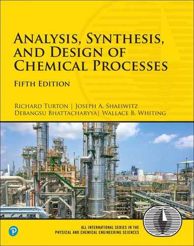
Figure 18.2(a) is a crude representation of a regulating or control valve. Fluid enters on the left of the valve. It flows under the valve seat, where it changes direction and flows upward between the valve seat and the disk. It again changes direction and leaves the valve on the right. The disk is connected to a valve stem that can be adjusted (in the vertical direction) by turning the valve handle. The position of the disk is given on the linear scale. The enlarged section shows the critical region involving the disk and the valve seat. The liquid flows through the annular space between the disk and the seat. As the disk is lowered, the area of this annulus decreases. The relationship between flowrate and valve position depends upon the shape of both the valve disk and the valve seat. It should be noted that the direction of flow through the valve could also be from the right to the left. In this case, the flow of the fluid pushes down on the disk and pushes it toward the seat. This configuration is preferred if the fluid is at a relatively high pressure or there is a large pressure drop across the valve.

Figure 18.2 Characteristics of Regulating Valves

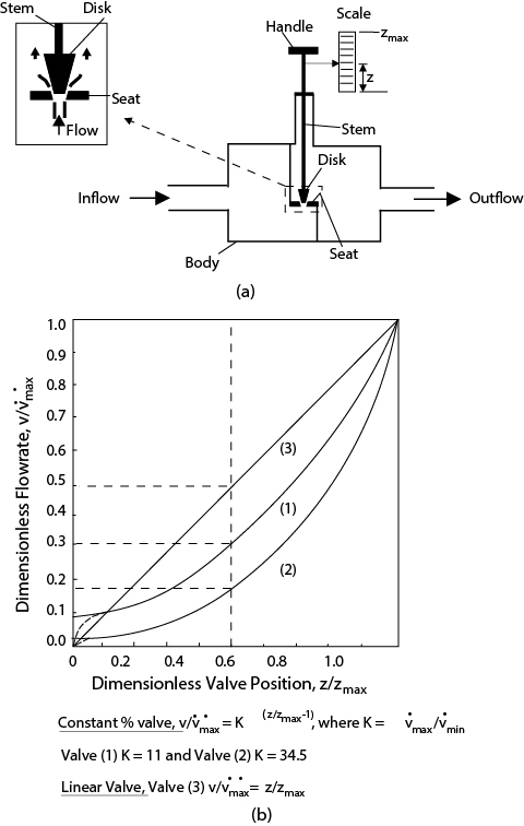
Figure 18.2(b) shows the pressure drop versus flowrate characteristics of regulating valves. To make a specific change in pressure drop across the valve, the valve must be opened or closed, as appropriate. In order to evaluate the desired valve position, it is necessary to know the performance diagram or characteristic for the valve.

Figure 18.3 is a mechanical drawing of the cross section of a globe valve. Globe valves are often used for regulation purposes. There are two general valve types used for regulation:

Figure 18.3 Cross Section of a Globe Valve (From McCabe, W. L. et al., Unit Operations of Chemical Engineering, 5th ed. (New York: McGraw-Hill, 1993), copyright © 1993 by McGraw-Hill Companies, reproduced with permission of the McGraw-Hill Companies)

Linear Valves. In a linear valve, the flowrate is proportional to the valve position. This is given by the relationship v˙=kz, where v˙ is the volumetric flow and z is the vertical position of the disk or valve stem.

Constant or Equal Percentage Valves. For an equal percentage valve, an equal change in the valve position causes an equal percentage change in flowrate. The valve equation for the constant percentage valve is given by v˙/v˙max=K(z/zmax−1). Note that a true constant percentage valve does not completely stop the flow. However, in reality, the valve does stop the flow when fully closed, and the constant percentage characteristic does not apply to very low flowrates, as indicated by the dashed lines at the lower end of the curves in Figure 18.2(b).

Both of these valve characteristics are described by the equations shown on Figure 18.2(b). Note that these equations strictly apply only for a constant pressure drop across the regulating valve. Example 18.1 illustrates the effect of using different valves.

Most valves installed are constant percentage valves, and there is no generally accepted standard design. Such valves offer fast response at high flowrates and fine control at low flowrates. The prediction of the disk position needed to give the required flowrate would be difficult using the performance diagram in Figure 18.2. In practice, the flowrate is controlled by observing a measured flowrate while changing the valve stem position. The valve position continues to be adjusted until the desired flowrate is achieved. This approach forms the basis of the feedback control system used for many automatic flow control schemes and discussed further in Section 18.5.

In practice, automatic control systems change valve positions to obtain a desired flowrate. The valve position is modified by installing a servomotor in place of the valve handle or by installing a pneumatic diaphragm on the valve stem.

18.3 Regulating Flowrates and Pressures

The rate equation describing the flowrate of a stream is given by

The driving force for flow is proportional to ΔP (pressure head), and the resistance to flow is proportional to friction. The resistance to flow can be varied by opening or closing valves placed in the flow path.

Figure 18.4 shows a pipe installed between a high-pressure header, containing a liquid, and a low-pressure header. The pressure difference, ΔP, between these two headers is the driving force for flow. Two valves are shown in the line, and when these valves are fully open, they offer little resistance to flow. The resistance in the transport line is due to frictional losses in the pipe. The flowrate is at a maximum value when the valves are fully open. When either valve in the line is fully closed, the resistance to flow is infinite, and the flowrate is zero. The valves may be adjusted to provide flows between these limits.

Figure 18.4 Pressure Profiles in a Pipe Containing Two Valves

Plotted below the diagram in Figure 18.4 are pressure profiles for various valve settings. The pressure (in kPa) is plotted on the y-axis, and it is noted that for the example shown P_in = 200 kPa and P_out = 100 kPa. The x-axis indicates the relative location of the valves in the process. In addition, Figure 18.4 includes a table that provides information on the flowrate, pressure drop due to pipe friction, and the pressure before valve CV-1. The resistance in the pipe is proportional to the square of the flowrate, which is the case for fully developed turbulent flow (see Chapter 19).

Profile 1 (a–f) shows the pressure profile with both valves fully open. It gives the maximum flowrate, 100 kmol/h, possible for this system. Profile 2 (a–b–c–f) is for the case when CV-1 is fully closed and CV-2 is fully open. For this case, the flow is zero, and all the pressure drop occurs over CV-1. The pressure upstream of CV-1 is P_in (200 kPa), and the downstream pressure is P_out (100 kPa). Profile 3 (a–d–e–f) is the case when CV-2 is fully closed and CV-1 is fully open. The pressure upstream of CV-2 is P_in (200 kPa), the downstream pressure is also equal to P_in (200 kPa), and the flowrate is zero.

For Profile 4 (a–g–h–f), valve CV-1 is partially open, providing a pressure drop of 45 kPa, and valve CV-2 is fully open. The pressure drop across CV-1 (ΔP_g-h) can be varied by changing the valve position of CV-1. The greater the pressure drop across CV-1, the lower the pressure drop available to overcome friction and the lower the flowrate. In Profile 4, the flow is reduced to 74% of the maximum flow.

For every setting of CV-1 (with CV-2 fully open), a unique value for pressure and flowrate is obtained.

Two valves are required to regulate simultaneously both the pressure and flowrate of a stream. The total system resistance (pipe and valves) determines the flowrate. The ratio of valve resistances establishes the pressure profile through the process. This is shown in Profile 5 (a–i–j–k–l–f), where 50% of the available pressure drop is taken over CV-1 and 31% is taken over CV-2. The resistance ratio for the two valves is 31/50 = 1.61, the flow is 44% of the maximum flow, and the pressure upstream of CV-1 is 194 kPa. To illustrate this concept further, consider Example 18.2.

Example 18.2

Consider the flow diagram in Figure 18.4. At design conditions, 70% of the total available pressure drop occurs across the two control valves, and the flowrate of fluid at these conditions is given as 100 [30/100]^0.5 = 54.8 kmol/h. If a point “z” that is midway between the two valves is considered, over what range can the pressure at point “z” be varied at the design flowrate?

To solve this problem, two extreme cases are considered: (1) CV-1 regulates the flow and CV-2 is fully open, and (2) CV-2 regulates the flow and CV-1 is fully open. Both these situations are illustrated in Figure E18.2. From Figure E18.2, it can be seen that the pressure at point “z” may vary between 185 kPa (CV-1 fully open) and 115 kPa (CV-2 fully open). Note that all possible combinations of partially open valves give pressures at point “z” between these two limits.

Figure E18.2 Range of Pressure at Point “z” for Design Flow

18.4 The Measurement of Process Variables

The process variables that are most commonly measured and used to regulate process performance are as follows:

• Temperature: Several instruments are available that provide continuous measurement of temperature—for example, thermocouples, thermometers, thermopiles, and resistance thermometric devices.

• Pressure: A variety of sensors are available to measure the pressure of a process stream. Many sensors use the deflection of a diaphragm, in contact with the process fluid, to infer the pressure of the stream. In addition, the direct measurement of process pressure by gauges—for example, a Bourdon gauge—is still commonly used.

• Flowrate: Fluid flowrates, until recently, were most often measured using an orifice or venturi to generate a differential pressure. This differential pressure measurement was then used to infer the flowrate. More recently, several other instruments have gained acceptance in the area of volumetric and mass flowrate measurement. These devices include vortex shedding, electromagnetic, ultrasonic, calorimetric, positive displacement, Coriolis, optical, and turbine flowmeters.

• Liquid Level: Liquid levels are commonly used in the regulation of chemical processes. There are many types of level sensors available, and these vary from simple float-operated valves to more sophisticated load cells and optical devices.

• Composition and Physical Properties: Many composition measurements are obtained indirectly. Physical properties such as temperature, viscosity, vapor pressure, electric conductivity, density, and refractive index are measured and used to infer the composition of a stream, in place of a direct measurement. A number of other measurement techniques have become commonplace for the on-line analysis of composition. These include gas chromatography and mass and infrared spectrometry. These instruments are very accurate but are expensive and often fail to provide the continuous measurements that are required for rapid regulation.

18.5 Common Control Strategies Used in Chemical Processes

There are many strategies used to control process variables in an operating plant. For more details, see Anderson [1] and Shinskey [2]. In this section, feedback, feed-forward, cascade, ratio, and split-range systems are considered.

18.5.1 Feedback Control and Regulation

The process variable to be controlled is measured and compared with its desired value (set-point value). If the process variable is not at the set-point value, then appropriate control action is taken.

Advantage. The cause of the change in the output variable need not be identified for corrective action to be taken. Corrections continue until the set-point value is achieved.

Disadvantage. No action is taken until after an error has propagated through the process and the error in the process variable has been measured. If there are large process lag times, then significant control problems may occur.

Example 18.3 illustrates the use of feedback control in a chemical process.

Example 18.3

Identify all the feedback control loops in the process flow diagram for the production of DME, in Appendix B, Figure B.1.1, and explain the control action of each. Note: There are other control valves on the utility streams, but these are shown only on the P&ID and not considered here.

All the control loops associated with the control valves shown on the PFD exhibit feedback control strategies. These are shown individually in Figure E18.3. Each control action is explained below.

Figure E18.3 Feedback Control Loops on DME Flowsheet

Figure E18.3(a): The objective of the controller is to control the flowrate of Stream 3, which is sent through two heat exchangers and then into reactor R-201. The flow sensed by the pressure cell (not shown) placed across the orifice in Stream 3 is used by the FIC to maintain the desired flow of Stream 3. However, because P-201 is a positive displacement pump, its flowrate should be maintained constant at the design flow. The discrepancy from the design flow gets reflected in the pump discharge pressure as shown by the pump curve in Figure 19.24. Therefore, the discharge pressure is maintainied by a control valve located on the bypass line.

Figure E18.3(b): The flowrate of the bottoms product in both distillation columns is adjusted to maintain a constant level of liquid in the bottom of the tower. The control strategies for the bottoms of both T-201 and T-202 are identical. Assume that the level in the bottom of the column drops below its set point. A signal from the level sensor would be sent to close slightly the valve on the bottoms product stream. This would reduce the flow of bottoms product and result in an increase in liquid inventory at the bottom of the column, causing the liquid level to rise. If the liquid level was to increase above the set-point value, then the opposite control action would be initiated.

Figure E18.3(c): The control strategy at the top of both columns (T-201 and T-202) is illustrated in Figure E18.3(c). The control action was explained previously in Example 18.1, where the reflux stream is held constant by a control valve and the liquid level in the reflux drum is held constant by adjusting the flow of the overhead product.

It should be noted that at present there is no product quality (purity) control on either column. This is addressed under cascade control below.

18.5.2 Feed-Forward Control and Regulation

Process input variables are measured and used to provide the appropriate control action.

Advantages. Changes in the output process variable are predicted, and adjustments are made before any deviation from the desired output takes place. This is useful, especially when there are large lag times in the process.

Disadvantages. It is necessary to identify all factors likely to cause a change in the output variable and to describe the process by a model. The regulator must perform the calculations needed to predict the response of the output variable. The output variable being regulated is not used directly in the control algorithm. If the control algorithm is not accurate and/or the cause of the deviation is not identified, then the process output variable will not be at the desired value. The accuracy and effectiveness of the control scheme are directly linked to the accuracy of the model used to describe the process.

Example 18.4 illustrates how feedback control, feed-forward control, or a combination of both can be used to control a process unit.

Example 18.4

Consider the process illustrated in Figure E18.4. The object is to cool, in a heat exchanger, a process stream (Stream 1) to a desired temperature (Stream 2) using cooling water supplied from a utility header. In Figure E18.4(a), a feedback control scheme is illustrated. The control strategy is to measure the temperature of the process stream leaving the heat exchanger (Stream 2) and to adjust the flow of cooling water to obtain the desired temperature. Thus, if the temperature of Stream 2 were to be greater than the desired set-point value, then the control action would be to increase the flow of cooling water and vice versa.

Figure E18.4 Control Strategies for Cooling a Process Stream

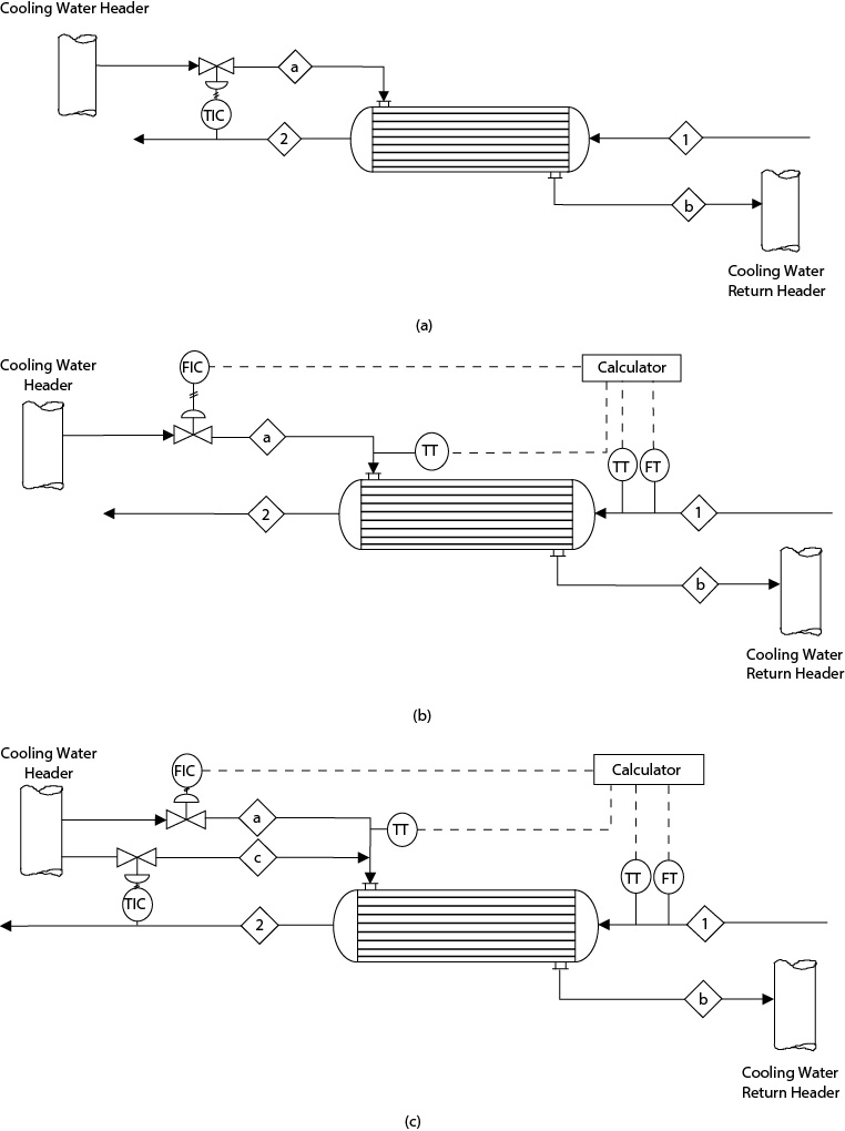
A feed-forward control scheme for this process is illustrated in Figure E18.4(b). Here, both the flowrate and temperature of the input process stream and the inlet cooling water temperature are measured. A calculation is then made that predicts the flowrate of cooling water needed to satisfy the energy balance and the exchanger performance equations as given in Chapter 20. Using the subscripts c and p to refer to the cooling water and process streams, respectively,

Q=m˙cCp,c(Tb−Ta)(E18.4a)

Q=m˙pCp,p(T1−T2)(E18.4b)

Q=UA(T1−Tb)−(T2−Ta)ln(T1−Tb)(T2−Ta)(E18.4c)

From Equations (E18.4a) through (E18.4c), the variables can be categorized as unknown, measured, known, and specified according to Table E18.4.

Table E18.4 Variables in Example 18.4

Unknown	Measured	Known	Specified
Q,m˙c,Tb	m˙p,Ta,T1	Cp,c, Cp,p, U, A	T2

Therefore, for a given value of the exit process temperature (T₂), Equations (E18.4a), (E18.4b), and (E18.4c) can be solved to give the unknowns in the table. Thus, by measuring the inlet process stream flow and temperature and the inlet cooling water temperature, the model given by Equations (E18.4a) through (E18.4c) can be solved to yield the desired value of the cooling water flowrate. The valve on the cooling water inlet can then be adjusted to give this value. There are some assumptions associated with this model that will affect the performance of this control scheme. The first assumption is that both streams flow countercurrently, and hence the exchanger effectiveness factor, F, is assumed to be equal to 1. If the value of F is not close to unity, then the model given above will not be accurate. However, the model can be modified by including another equation to calculate F based on the process variables. A more restrictive assumption is that the overall heat transfer coefficient, U, has a constant value. In real processes, this is seldom the case, either because of flowrate changes or due to fouling of heat-exchange surfaces occurring throughout the life of the process. As the heat transfer surfaces foul or flowrates change, the value of U changes and the predictions of the above model will deviate increasingly from the true value of T₂. This illustrates one of the major disadvantages of feed-forward control strategies, in that the efficacy of the control strategy is only as good as the predictions of the equations used to model the process.

An alternative scheme to pure feed-forward control is to use a combination of feedback and feed-forward control strategies. This is illustrated in Figure E18.4(c) and discussed in Section 18.5.3.

18.5.3 Combination Feedback and Feed-Forward Control

By correctly combining these two control strategies, the advantages of both methods can be realized. The feed-forward strategy uses measured input variables to predict changes necessary to regulate the output. The feedback regulator then measures the regulated output variable and makes additional changes to ensure that the process output is at the set point.

Advantages. The advantages of both feedback and feed-forward regulation are achieved. The feed-forward regulator makes the major corrections before any deviation in process output takes place. The feedback regulator ensures that the final set-point value is achieved.

Disadvantages. The control algorithm and hardware to achieve this form of control are somewhat more complicated than either individual strategy.

Example 18.5 considers the operation of the combination of feedback and feed-forward control.

18.5.4 Cascade Regulation

The cascade system uses controllers connected in series. The first control element in the system measures a process variable and alters the set point of the next control loop.

Example 18.6

Consider the control of the top-product purity in distillation column T-201 in the DME process. As shown in Example 18.3, the material balance control is achieved by a flow controller on the reflux stream and a level controller on the top product stream. From previous operating experience, it has been found that the top-product purity can be measured accurately by monitoring the refractive index (RI) of the liquid product from the top of the column, Stream 10. Using a cascade control system, indicate how the control scheme at the top of T-201 should be modified to include the regulation of the top-product composition.

The solution to the problem is illustrated in Figure E18.6. An additional control loop has been added to the top of the column that consists of a refractive index measuring element that sends a signal to the flow controller placed on the reflux stream (Stream 16). The purpose of this signal is to change the set point of the flow controller. Consider a situation where the purity of the top product has decreased below its desired value. This change may be due to a number of reasons; for example, the flowrate or purity of the feed to the column may have changed. However, the reason for the change is not important at this stage. The decrease in purity will be detected by the change in refractive index of the liquid product, Stream 10, and a signal will be sent from the RI sensor to increase the reflux flowrate of Stream 16. The flow of Stream 16 will increase, which will result in an improved separation in the column and an increase in purity of the top product. For an increase in product purity, the reverse control action will occur.

Figure E18.6 Cascade Control for DME Overhead Product Purity

18.5.5 Ratio Control

In a number of process systems, it is desired to maintain the ratio between two variables such as concentrations or flowrates. Ratio control has been applied to both reacting and nonreacting systems. Examples of reacting systems include the water-gas shift (WGS) reactors where the H₂O/CO ratio is maintained at some optimum value, the Claus unit where a desired H₂S/SO₂ ratio is maintained at the Claus reactor inlet, and combustors where a desired (C + H₂)/O₂ ratio is maintained to ensure very low levels of CO in the combustion product stream. Examples of nonreacting systems include slurry-fed systems where the ratio of the flowrate of the liquid to the flowrate of the solids must be maintained at some value to ensure the flowability of the slurry, steam atomization of burners where the steam-to-fuel flowrate is maintained for desired atomization, and systems where two streams are mixed to modify the physical properties of one of the streams such as its surface tension, viscosity, density, and so forth.

Advantages. Ratio control is a special type of feed-forward control system in which a ratio is maintained to achieve a desired control objective. Therefore, this strategy has all the advantages of a feed-forward control system but without the need of a process model, which is a requirement for feed-forward control.

Disadvantages. The main assumption used in ratio control is that the controlled ratio is the key variable, so that if it is maintained at a desired set point, the control objective will be satisfied. However, there may be other variables that play a significant role in a given operating region. For example, for a water-gas shift (WGS) reactor, the H₂O/CO ratio might be maintained at the inlet to obtain a desired conversion of CO in the system. However, the actual conversion of CO depends upon many other variables such as residence time, catalyst activity, presence of other impurities, and so on. Thus, the actual control objective may not be satisfied by ratio control alone. The advantages and disadvantages of ratio controllers are investigated further in Example 18.7.

Example 18.7

Consider the first water-gas shift (WGS) reactor shown in Figure B.12.1. It is desired to maintain the H₂O/CO ratio at the inlet of the first WGS reactor at a given value. The flowrate of the steam, Stream 4, can be manipulated to achieve the desired ratio. However, the pressure of Stream 4 is known to vary. Develop two control configurations to control the H₂O/CO ratio (R_SP). What are the advantages and disadvantages of each of the control configurations?

Solution

Figures E18.7(a) and E18.7(b) show two possible control strategies. In Figure E18.7(a), the flow of the syngas and its composition (CO and H₂O) are measured. Then the desired flowrate of Stream 4 required to achieve the desired ratio is calculated. If the molar flowrate of Streams 3 is F₃ and the concentrations of CO₂ and H₂O in Stream 3 are yCO2 and yH2O, respectively, then the set point for the steam flow controller, F_SP, can be calculated to achieve R_SP, the desired H₂O/CO ratio.

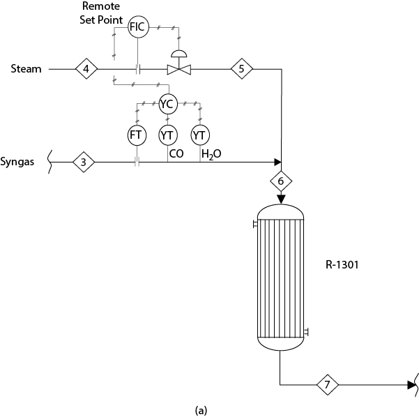
Figure E18.7(a) Ratio Control Strategy of a WGS Reactor System Where the Inlet Flowrate to the System is Measured

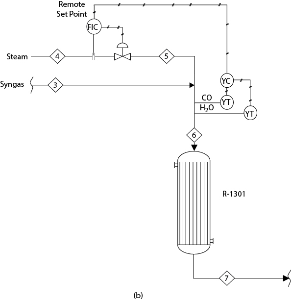
Figure E18.7(b) Ratio Control Strategy of a WGS Reactor System Where the Inlet Flowrate Is Not Measured

FSP=F3(yCORSP−yH2O)

Since the steam pressure is known to vary, a cascade control strategy is considered so as to reject the disturbances in the steam flow due to the varying steam header pressure. The advantage of this ratio control strategy is that the desired flowrate of the steam can be exactly calculated. The disadvantage is that the flowrate and composition of the syngas has to be measured.

In the second strategy, shown in Figure E18.7(b), the flow of the steam is again set by a flow indicator controller (FIC). However, in this case, the set point of the FIC is adjusted so as to maintain the desired H₂O/CO measured at the reactor inlet. Therefore, in the control strategy shown in Figure E18.7(b), the composition (CO and H₂O) at the inlet of the reactor is measured and the flowrate of the steam is manipulated by a feedback mechanism. The performance of this control strategy depends upon the tuning of the ratio controller as the exact set point F_SP cannot be calculated.

18.5.6 Split-Range Control

A split-range control strategy is used when a single manipulated variable (MV) is not sufficient to maintain the controlled variable (CV) at its set point. Split-range control can be used for both servo and regulatory controls. In the case of servo control, split-range control is used when the set point varies over a wide range such that it cannot be maintained with a single MV. A split-range control strategy is also used for regulatory control, where a single MV fails to reject the entire range of disturbances. Split-range control strategies vary based on how the control valves open and close in response to the split-range controller. For example, if there are two control valves, A and B, then the following strategies may be considered:

Split-Range Strategy 1: At 0% output of the split-range controller, control valve A is 100% open and B is closed. As the split-range controller output increases from 0% to 100%, control valve A closes and control valve B opens. At 100% output of the split-range controller, control valve B is 100% open and A is fully closed.

Split-Range Strategy 2: At 0% output of the split-range controller, control valve A is 100% open and B is closed. As the split-range controller output increases from 0% to x% (x < 100; the value of x is often chosen to be 50), control valve A closes whereas control valve B remains closed. At x% output of the controller, both control valves are completely closed. As the controller output increases from x% to 100%, control valve B opens and reaches 100% open at 100% of the controller output. During this time, control valve A remains closed.

Split-Range Strategy 3: At 0% output of the split-range controller, both control valves are fully closed. As the controller output increases from 0% to x% (x < 100; the value of x is often 50), control valve A opens and becomes fully open when the controller output reaches x%. On the other hand, during this time, control valve B remains closed. As the controller output increases from x% to 100%, control valve B opens and becomes 100% open at 100% of the controller output. During this time, control valve A remains fully open.

Advantages. A split-range controller is required to avoid input saturation or to achieve satisfactory control over a wide operating region.

Disadvantages. Controller tuning can be very difficult as the process gain and transients for each of the inputs can be very different.

Example 18.8 shows the use of a split-range controller for servo control using Split-Range Strategy 1.

Example 18.8

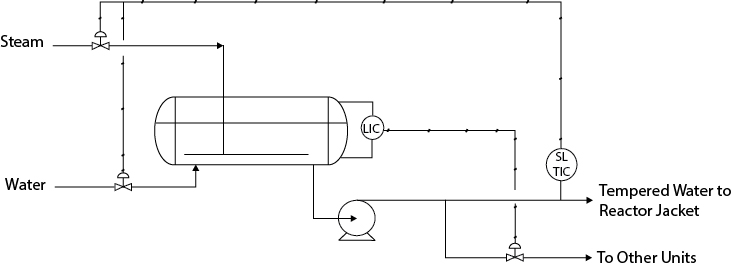
A tempered-water system is used for maintaining the temperature of a batch reactor. The set point for the tempered water varies between 45°C and 90°C. Feed water is available at 40°C, and steam is available at 120°C. Develop a split-range control configuration to maintain the temperature of this tempered-water system.

Figure E18.8 shows the split-range control configuration. When the set point is 45°C, the steam control valve is open a small amount. As the set point increases, the water control valve keeps closing while the steam control valve starts to open. When the set point is 90°C, the steam control valve is fully open, while the water control valve will be at some minimum open value. In this example, a modified Split-Range Strategy 1 is being used. In this strategy, the water and steam valves are clamped so that a minimum flow of each stream will occur at the extreme limits of the controller to maintain the correct energy balance.

Figure E18.8 Temperature Control of a Tempered-Water System Using Split-Range Control

Example 18.9 shows a split-range control strategy for regulatory control using Split-Range

Strategy 2.

Example 18.9

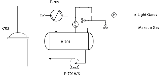
Figure B.6.1 shows the process for ethylene oxide production. Noncondensable light gases are vented from V-701. The amount of this gas at steady-state design conditions is very low. During plant operation, it is known that the amount of noncondensable gas in V-701 varies. Devise a split-range control strategy where the pressure of V-701 can be maintained at its steady-state design value even though the amount of noncondensable gas becomes negligible or higher than the design value.

The split-range control strategy is shown in Figure E18.9, where Split-Range Strategy 2 is used. Under the design condition, light gases are vented from V-701; consequently, only the vent valve (in Stream 34) remains open. If the pressure keeps decreasing, then its set point, the split-range controller output, keeps decreasing. This causes the vent valve to close gradually, being fully closed at 50% of the controller output. If the pressure decreases further, the split-range controller output decreases further. As a result, the control valve for makeup gas starts opening and becomes fully open at 0% of the controller output. The vent and makeup control valves should be designed considering the extremes of the flow of noncondensable gases in the system.

Figure E18.9 Split-Range Pressure Control of the EO Column Reflux Drum in Ethylene Oxide Production

These control strategies do not represent a comprehensive list of possibilities. The range of strategies is very large. This is due, in part, to the flexibility that software has added to the control field by allowing sophisticated process models to be used in simulating processes, as well as the use of more complicated control algorithms.

No mention has been made of the types of controller (proportional, differential, integral, etc.) and strategies to tune these controllers. Such information is covered in traditional process control texts, such as Stephanopolous [3], Coughanowr [4], Smith and Corripio [5], Seborg et al. [6], and Marlin [7].

18.6 Exchanging Heat and Work between Process and Utility Streams

In order to obtain the correct temperatures and pressures for process streams, it is often necessary to exchange energy, in the forms of heat and work, with utility streams. In order to increase the pressure of a process stream, work is done on the process stream. The conversion of energy (usually electrical) into the pressure head is provided by pumps (for liquid streams) or compressors (for gas streams) that are inserted directly into the process stream. For a process gas stream undergoing a significant reduction in pressure, the recovery of work using a gas turbine may have a significant impact (favorable) on process economics. In order to change the temperature of a process stream, heat is usually transferred to or from a process by exchange with a heat transfer medium—for example, steam and cooling water. As shown in Chapter 15, it may also be beneficial for heat to be exchanged between process streams using heat integration techniques.

18.6.1 Increasing the Pressure of a Process Stream and Regulating Its Flowrate

In the preceding examples, streams were available at constant pressure. This is normally true for utility streams. However, for a process stream, the pressure may change throughout the process. When higher pressures are needed, pumps or compressors are installed directly into a process stream. These units convert electrical energy into the required pressure head for the stream.

It should be noted that when a pump or compressor is required in a process, it is necessary to specify the type of fluid and fluid conditions, the design flowrate of fluid, the inlet (suction) and outlet (discharge) pressures at the design conditions, and an overdesign (safety) factor. The pump or compressor conforming to these specifications must be able to operate at and somewhat above the design conditions. However, in order to regulate the flow of the process streams, as will be required throughout the life of the process, it is necessary to implement a control or regulation system. Some typical methods of regulating the flow of process streams are outlined below and shown in Figure 18.5.

Figure 18.5 Flowrate Feedback Control Schemes for Pumping Liquids

Figure 18.5(a) shows a centrifugal pump system that increases the pressure of a process stream. The position of the control valve, CV-1, is at the discharge side of the pump. The flowrate of Stream 2 is changed in order to regulate the flow of the stream passing through the pump. The operation of the pump and the interaction of the pump curve, the system curve, and the control valve will be discussed in the presentation of pump performance curves in Chapter 19. In reviewing this material, it is important to remember that the maximum flowrate of the fluid is determined by the intersection of the pump and system curves. Regulation of flowrate is possible only for flows less than this maximum value, that is, to the left of the intersection of the pump and system curves, as illustrated in Figure 19.22.

Figure 18.5(b) shows a positive displacement pump increasing the pressure of a process stream. The positive displacement pump can be considered to be a constant-flow, variable-head device; that is, it will deliver the same flowrate of fluid at a wide range of discharge pressures. Thus

Under design condition, a small amount of flow is usually recycled for easier operability. During process operation, if the flow of the process stream, Stream 2, decreases below the design flow, the recycle flowrate, that is, the flowrate of Stream 3, must be increased to ensure that the total flowrate remains constant. In Figure 18.5(b) this is accomplished by returning Stream 3 through CV-2 to the suction side of the pump. Flow regulation of Stream 2 is accomplished by manipulating CV-3 placed on Stream 2. It should be noted that the pump curve of a positive displacement pump is almost vertical and even with minor changes in the flow due to throttling of the control valve on Stream 2, the discharge pressure will increase drastically (see Figure 19.24). Therefore the pump discharge pressure can be used as a surrogate measurement to capture the discrepancy from the design flow. CV-2 is manipulated to maintain the pressure by regulating the recycle flowrate.

Figure 18.5(c) uses a variable-speed drive—or variable displacement volume, for a positive displacement pump—to regulate the flow of the process stream. For a centrifugal pump, the impeller speed is regulated to provide the required flow, at the desired pressure, for the process stream. The advantage of using this type of control strategy is that there is no wasted energy due to throttling across a control valve. However, variable-speed controls and motors are expensive and less efficient. Therefore, this type of control scheme is usually cost effective only for gas blowers, compressors, and large liquid pumps, because a large savings in utilities is required to offset the large capital investment for the variable-speed drives and controls.

Figure 18.5(d) regulates the input flow with a valve, CV-4, installed in the suction line to the pump. The position of CV-4 is altered to provide the desired flowrate of fluid. This may work well for gases (suction throttling of blowers and compressors) but is seldom used for liquid pumps. For liquid streams, the reduction in pressure at the pump inlet increases the possibility of cavitation; that is, NPSH_A is reduced drastically. The causes of cavitation and NPSH calculations will be covered in Section 19.5.2. On the other hand, for the case of gas compression using centrifugal machines, the throttling of the inlet stream is essential for start-up purposes. Thus, this method is often the preferred control strategy for flow regulation in centrifugal blowers and compressors.

All the control systems shown in Figure 18.5 for the regulation of liquid process streams can be applied to compressor systems to regulate the flow of gaseous process streams.

18.6.2 Exchanging Heat between Process Streams and Utilities

The amount of heat added to or removed from a process stream is usually altered by changing the flow or pressure of utility streams. The primary utility streams in a chemical plant are as follows:

1. Cooling water is used to remove heat from a process stream. The heat transferred to the coolant adds to the sensible heat (enthalpy) of the coolant stream (temperature increases).

2. Air can be used to remove heat from a process stream and is often used in product coolers and overhead condensers. The heat transferred to the coolant adds to the sensible heat (enthalpy) of the coolant stream (temperature increases).

3. Steam condensation is used to add heat to a process stream. The heat transferred from the steam decreases the enthalpy of the steam (steam condenses).

4. Boiler feed water (bfw) is used to remove heat from a process stream to make steam that can be used elsewhere in the process. The heat transferred to the bfw increases the enthalpy of the bfw stream (bfw vaporizes).

When using cooling water or air in which there is no change of phase of the utility stream, regulation is generally performed by changing the flowrate of the cooling stream. For example, see Figure E18.4 and Example 18.4. In this section, the focus is on systems in which the utility stream undergoes a change of phase. The focus is on boiler feed water and steam. However, the results apply equally well to other heat transfer media that undergo a phase change. It is further assumed that utility streams are taken from and returned to headers and that the process streams are a single phase. The control of reboilers and condensers in a distillation column is covered in the case study on distillation given in the following section.

There are many ways to regulate systems using steam. No effort is made here to try to present an exhaustive list of possible schemes, but the focus is on several of the more common techniques. Figures 18.6 and 18.7 show several systems used to control the transfer of heat between a utility stream and a process stream. The systems on the left-hand side of the figures add heat to the process stream by condensing steam. Systems on the right-hand side remove heat from the process stream by vaporizing bfw. In either case, there are two phases present in equilibrium on the utility side of the exchanger. The temperature and pressure are related by the vapor-pressure relationship for water. If steam from the header is significantly superheated, it may be passed through a desuperheater prior to being fed to the heat exchanger. The desuperheater adds just enough bfw to saturate the steam. The reason for using a desuperheater is that highly superheated steam acts like a gas with a correspondingly low film heat transfer coefficient. Thus, a significant amount of heat-exchanger area may be taken up in desuperheating the steam. In such situations, it is more cost effective to saturate the steam before entering the heat exchanger, reducing significantly the heat exchange area required.

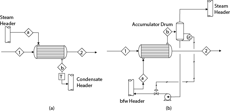
Figure 18.6 Unregulated Heat Exchanger Using Utility Streams with a Phase Change: (a) Process Heater and (b) Process Cooler

Figure 18.7 Regulation Schemes for a Heat Exchanger Using Utility Streams with a Phase Change

Figures 18.6(a) and 18.6(b) show a process heater (steam condenser) and a process cooler (bfw vaporizer) without control valves. The heater shown in Figure 18.6(a) includes a steam trap (shown as a box with a T in the middle) on the utility line. This steam trap separates the condensate formed from the vapor. The condensate is collected by the trap in the bottom of the exchanger and discharged intermittently to the condensate header. The steam flowrate, Stream a, is established by the rate at which heat is exchanged. This is different from normal utility flow regulation. As the steam condenses, there is a large decrease in the specific volume of the utility stream. Thus, steam is continually “sucked” from the header into the heat exchanger. For this system, no regulation of process temperature is attempted.

The process cooler shown in Figure 18.6(b) vaporizes bfw. In this case, the flow of bfw is more than sufficient to provide for the vaporization taking place. The exit stream is a two-phase mixture of steam and bfw. The bfw is separated from the vapor in an accumulation drum (phase separator) and recycled back to the inlet of the exchanger. Again, for this system, no regulation of process temperature is attempted.

Although no control schemes are implemented in the systems in Figure 18.6(a)(b), to some extent, both systems are self-regulating. The reason for this self-regulating property is that the major resistance to heat transfer is on the process side (film heat transfer coefficients for condensing steam and vaporizing bfw are very high). Consider an increase in the flowrate of the process stream in Figure 18.6(a). As the flow increases, so does the process-side heat transfer coefficient, and, for turbulent flow, this increase is proportional to the (process flowrate)^0.8–0.6. See Table 20.8 for an explanation of the range of exponents. Because the major resistance to heat transfer is on the process side, this suggests that the overall heat transfer coefficient changes by the same amount. Thus, for a 10% increase in process flowrate, the overall heat transfer coefficient increases by 6% to 8%. Because the change in the overall heat transfer coefficient does not quite match the change in process flowrate, the exit temperature of the process stream, Stream 2, must drop slightly. Although the temperature of the exit stream drops, it does not drop by much due to the partial regulation provided by the increase in heat transfer coefficient.

In discussing the operation of this heat exchanger, no mention was made of the change in flowrate of the steam that would be required to provide the increase in heat-exchanger duty caused by the increased process flowrate. As the exchanger duty increases, more steam will condense, and this increased demand for steam does have an effect on the operation. It should be noted that steam is supplied from the header to the exchanger in the quantity that is required; that is, it is determined by the energy balance. As the steam flowrate increases, the frictional pressure losses in the supply pipe from the header to the exchanger increase. This causes the pressure on the steam side of the heat exchanger to decrease. Thus, the utility side of the heat exchanger essentially “floats” on the header pressure, with an appropriate pressure loss to account for flow through the supply line. As the pressure of the steam side of the exchanger drops, this causes the temperature at which the steam condenses to drop slightly, thus reducing the temperature driving force for heat exchange. However, compared with the change in heat transfer coefficient, this change is minor.

In order to regulate the temperature of the process stream leaving the heat exchanger, it is necessary to control the heat duty. In order to do this, a variable on the right-hand side of the heat-exchanger performance equation must be able to be regulated:

This can be achieved by doing one or more of the following:

1. Regulate the temperature driving force (ΔT_lm) between the process fluid and the utility.

2. Adjust the overall heat transfer coefficient (U) for the heat exchanger.

3. Change the area (A) for heat exchange.

Two alternatives are considered for regulating the temperature of the process exit stream.

Regulate the Temperature Driving Force between the Process Fluid and the Utility. The systems shown in Figure 18.7(a)(b) include a valve on the utility line. This valve is used to change the pressure of the utility stream in the exchanger. Because there are two phases present, the pressure establishes the temperature at which the phase change takes place. Reducing pressure reduces temperature according to the vapor-pressure-temperature relationship for water, for example, from Antoine’s equation.

To increase the heat duty for the process heater, Figure 18.7(a), the temperature driving force is increased by increasing the pressure. This is achieved by opening CV-1 to decrease the frictional resistance to flow. Because CV-1 is located on the input side of the heat exchanger, opening the valve increases the pressure of the steam in the exchanger, and the temperature at which condensation occurs will also increase. To increase the process cooler heat duty, Figure 18.7(b), the temperature driving force is increased by opening CV-2, which decreases the resistance to flow. CV-2 is located on the discharge side of the utility, that is, between the exchanger and the steam header. In this case, the exchanger once again floats on the steam header pressure. As CV-2 is opened, the pressure on the utility side of the exchanger decreases, and this reduces the temperature at which the bfw boils and increases the temperature driving force for heat transfer.

Adjust the Overall Heat Transfer Coefficient for the Heat Exchanger by Adjusting the Area Exposed to Each Phase. The systems shown in Figure 18.7(c)(d) operate such that the interface between the liquid and vapor on the utility side of the exchanger covers some of the tubes. For this situation, a fraction of the heat-exchange area is immersed in the liquid region, with the remaining fraction in the vapor-phase region. The heat transfer coefficients and the temperature driving forces for these two regions differ significantly. Thus, by adjusting the level of the liquid-vapor interface in the exchanger, it is possible to regulate the duty.

For the process heater, Figure 18.7(c), decreasing the level increases the heat duty. The reason for this is that in the vapor-phase region the utility-side film coefficient and temperature driving force are large because steam is condensing. For the liquid-phase region, both the film coefficient and temperature driving force are low because the condensate is being subcooled. Therefore, as the liquid level decreases, more heat transfer area is exposed to condensing steam, the overall average value of UA increases, and the duty increases.

For the process cooler, Figure 18.7(d), increasing the liquid level increases the heat duty. The reason for this is that in the vapor-phase region, the utility-side film coefficient and temperature driving force are low because steam is being superheated. For the liquid-phase region, both the film coefficient and temperature driving force are high because the bfw is boiling. Therefore, as the liquid level increases, more heat transfer area is exposed to boiling water, the overall average value of UA increases, and the duty increases. Careful consideration of the disengagement height must be made in the design of these steam generators to ensure that free water does not get into the steam header even at the maximum allowable level and the maximum velocity of the generated steam.

18.6.3 Exchanging Heat between Process Streams

The integration of heat between process streams is often economically advantageous, and a strategy to do this is explained in Chapter 15. When heat integration is implemented in a process, it is unlikely that the flow of these process streams can be regulated to control the heat transfer, because these flows may be set based on the operation of other critical equipment items and/or plant throughput. Rather the flowrates, composition, temperature, and vapor fraction of these streams can change due to changes in the process operation. One method to control the exit temperature in such an exchanger is to bypass some portion of one or both of the process streams around the exchanger. By altering the amount of the stream that bypasses the equipment, temperature regulation is possible. This concept is considered further in Problem 18.4.

18.7 Logic Control

Logic control, often neglected in traditional undergraduate curricula, is an inseparable part of the overall control system design of a modern plant. Logic control executes logical steps and implements its decisions. Logic controllers are used in batch, continuous, and semibatch processes. In Chapter 3, a number of examples were given that show the various steps involved in a typical batch process. A logic controller carries out this sequence of steps in a batch process and repeats them based on some preprogrammed condition(s). In continuous processes, logic controllers are used for plant/equipment safety and for avoiding interruption in plant operation in the case of failure of an equipment/section of a plant. Logic controllers ensure that the start-up conditions for an equipment/plant section (known as start permissives) are satisfied before an equipment/plant section is permitted to start. Moreover, logic controllers continuously monitor various equipment/plant sections to avoid unsafe or dangerous situations and implement a series of preprogrammed steps in case of a shutdown. In a semibatch process, logic controllers usually execute a series of steps for smooth switching between two or more reactors/beds/process equipment at a regular interval. The platform in which the logic control system is usually implemented in industry is known as a programmable logic controller (PLC). The programming language for a PLC varies depending on the manufacturer. Examples of programming languages include Ladder Diagram (LD), Structured Text (ST), Sequential Function Chart (SFC), Function Block Diagram (FBD), and Instruction List (IL). LD is the most widely used language. Most of these programming languages follow the IEC-61131 standard. A single PLC can be used for implementing logic control of a number of equipment/process sections. Some manufacturers of special equipment such as turbines, compressors, and furnaces have dedicated PLCs for their equipment. Otherwise, even for large process plants, a single or a few PLCs may be sufficient. A brief discussion of LD will be provided, because of its popularity in the process industries.

Components of LD. An LD looks like a ladder—hence the name—where some logical processing is carried out at each “rung.” An LD can span several thousands of rungs. The components of an LD are of three types: input devices or contacts, internal devices, and output devices or coils. Each rung usually starts with one or more contacts and terminates in one or more coils directly or through one or more internal devices. Based on the state of the input devices (true or false) and the mathematical/logical operation carried out in the internal devices, the state of the output device becomes true (i.e., energized) or false (i.e., deenergized). The state of the input devices can be altered (i.e., true or false) by field instruments (such as start/stop switches, level switches, etc.) or by internal flags that are generated by the output device(s). When the output device becomes energized or deenergized, it can operate some field equipment (such as start/stop a motor, open/close valves, etc.), or it can change the status of some internal flags. Contacts can be used as internal devices as well. A few basic components of an LD are shown in Figure 18.8. Figure 18.8(a) represents a contact that is normally open (NO). Its state can be altered by a flag such as a motor start switch, a limit switch, or any internal flag. For example, if a motor start switch changes the state of an NO contact, then initially the output of this contact is false or 0. As the motor start button is pressed, the contact becomes closed, changing its state to true or 1. Figure 18.8(b) represents a contact that is normally closed (NC), that is, normally true. Its status can be changed to false by a flag as before. Figure 18.8(c) represents an internal device known as one-shot rising (OSR) that can be used to trigger a one-time event. When the input to the OSR becomes true, its output becomes true for one cycle, then becomes false in subsequent scans unless its input changes to true again. Figure 18.8(d) shows a coil that becomes true when its input flag is true. Figure 18.8(e) shows an output latch that becomes true when its input becomes true. It then remains true even when its input turns false. The output is triggered false when it is unlatched by an “output unlatch,” shown in Figure 18.8(f). Many other components are used in an LD. Examples include timer on/off delay, various comparators, function blocks, and various mathematical operations that can be used to turn a signal on or off. For a detailed discussion of these topics, refer to one of the many good books in this area [8–10].

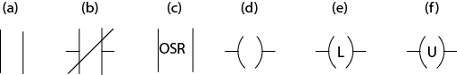
Figure 18.8 Basic Components of an LD: (a) Normally Open (NO) Contact; (b) Normally Closed (NC) Contact; (c) One-Shot Rising; (d) Coil; (e) Output Latch; (f) Output Unlatch

Example 18.10

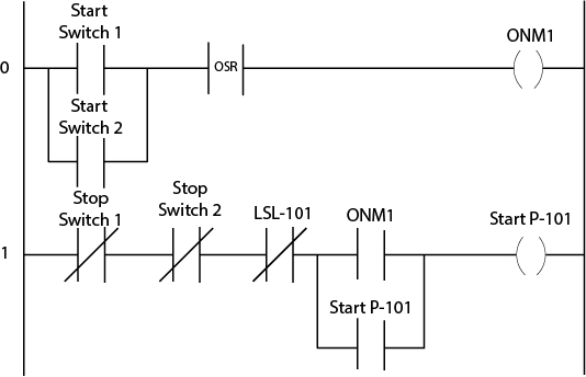
Figure E18.10(a) shows the schematic of a storage vessel, V-101. Pump P-101 has two start and stop switches (one in the plant and the other in the control room). Assume that the pump start switch is a momentary signal, that is, is true as long as the start button is pushed. The pump can be started or stopped by either of the start/stop switches. Pump P-101 should stop if the level of the vessel becomes low as detected by the level switch, LSL-101. Develop a ladder diagram for the pump.

Figure E18.10(a) Schematic of a Storage Vessel

The ladder diagram is shown in Figure E18.10(b). In Rung 0, if any one of the pump start switches is pressed, it generates a true flag, making the OSR output to be true for only one cycle. This makes the output of ONM1 true. If any of the stop switches and LSL-101 are not true, then when ONM1 is true, a pump start signal, Start P-101, is generated in Rung 1. This start signal is usually sent to a motor control center (MCC) located in an electrical substation to start the pump. As the OSR output is true only once when any of the pump start switches is true, ONM1 will be false at the next scan and the pump will turn off. To prevent this, the Start P-101 signal is used in parallel to ONM1. While the pump is running, if any of the stop switches is pressed or the LSL-101 is activated due to low level, the input to the Start P-101 contact becomes false and trips the pump.

Figure E18.10(b) Ladder Diagram for Pump Start/Stop

18.8 Advanced Process Control

Advanced process control (APC) involves many tools from process control theory. This term broadly covers advanced techniques employed for process control applications. APC is very effective for process systems under a number of circumstances such as the following:

• When multivariable interactions prohibit satisfactory control performance with a single-loop control

• When the process dynamics are so complex that a traditional control fails to give acceptable performance

• When the control system must satisfy some desired dynamic behavior

• When there are process constraints that cannot be violated under any circumstances

• When the control objective is to optimize some function, such as maximize profit, minimize auxiliary power consumption, and so forth, that involves multivariable interactions and (often) explicit process constraints

• When consistent product specifications cannot be met with traditional control

• When the plant operation is desired to be highly flexible

Nonetheless, APC is an umbrella term for a number of process control techniques. Based on their popularity, two such techniques will be briefly discussed here.

18.8.1 Statistical Process Control (SPC)

In this category, statistical methods are applied for process control. Quality control is one of the main focuses of SPC, ensuring that the product qualities are satisfied consistently in the face of inherent variability. In SPC, the process is monitored by using a quality control chart such as the Shewart chart, CUSUM (Cumulative Sum) chart, or other similar technique. In the case of undesired deviation of a process variable from its desired value, an objective analysis is carried out to determine the root cause by using techniques such as Ishikawa diagrams, Pareto charts, and other such tools. A control action is then taken to eliminate the root cause. SPC is primarily used in the manufacturing industry where the costs of making such adjustments are large and the process is not subject to persistent disturbances. In the process industry, usually the cost of making adjustments is minimal and the disturbances are not only persistent but significant. Therefore, SPC has fewer applications in the process industry.

18.8.2 Model-Based Control

In model-based control, a process model is used to decide the appropriate control action. Two approaches are very popular in this category. In the first approach, known as the direct synthesis approach, the controller is designed to follow a desired trajectory. Two common techniques are internal model control and generic model control. The other approach is known as optimal control, where the controller is designed to optimize some objective function, quite often subject to some constraints. Model Predictive Control (MPC) is probably the most popular control scheme in this category. In linear MPC, a linear process model is used to predict the future process trajectory over a time horizon known as the prediction horizon. The control action is then calculated over a time horizon known as the control horizon by carrying out an optimization. Popular methods under this category are linear quadratic control (LQC), dynamic matrix control (DMC), and model algorithmic control (MAC). For systems that cannot be well represented by a linear model, a nonlinear process model is necessary, leading to nonlinear MPC. The optimization problem in a linear MPC can be solved by very efficient algorithms available for solving quadratic programming (QP) problems. However, nonlinear MPC leads to a nonlinear programming (NLP) problem that can be computationally expensive for large and complicated process systems. Another issue with any model-based control is to obtain a representative process model. When a representative first-principles process model is available, it can be used. When such models are not available, the actual process is excited by an appropriately designed input signal, and a process model is identified using the process response. The performance of an MPC application can significantly deteriorate if the actual process deviates considerably from the model over the course of time. In such cases, the identification of an updated process model is required. To obtain satisfactory control performance in the face of model/parametric/input/output uncertainties is the focus of robust process control, which is an active field of research. Another problem for any APC application is its maintenance because complicated process control theory is usually involved.

Many other APC techniques are available in the existing literature. Readers interested in these techniques and the theory and applications of APC techniques are referred to a number of good references in this area [11–13].

18.9 Case Studies

In this section two operations that require more complex control schemes are studied in detail. Again, it is emphasized that these are not the only ways to control these units but are typical schemes that might be employed. Many alternatives exist, and in the course of a career in process engineering, you will encounter a wide variety of regulation systems.

18.9.1 The Cumene Reactor, R-801

Consider the reactor system for the production of cumene shown in Appendix C, Figure C.8, and redrawn in Figure 18.9. The reactor feed, Stream 7, comes from a fired heater, where it is heated to the temperature required in the catalytic reactor. The reaction takes place in a bank of parallel catalyst-filled tubes and is mildly exothermic. In order to regulate the temperature of the reacting mixture and catalyst, the tubes are immersed in boiler feed water. The heat is removed by vaporizing the water to make high-pressure steam, which is then sent to the high-pressure steam header.

Figure 18.9 Basic Regulation Scheme for Cumene Reactor, R-801

The first issue is what should be controlled in the reactor and why. This is not a simple question to answer because many things must be considered. Some of the important considerations for exothermic catalytic reactions are discussed in Chapter 22. Here, it is assumed that the exit temperature from the reactor, Stream 8, is the variable that must be controlled. If the reactor is designed such that the temperature increases monotonically from the inlet to the outlet, then the exit stream is the hottest point in the reactor. More commonly, there will be a temperature bump or warm (hot) spot somewhere within the reactor, and the exit temperature will be cooler than at the temperature bump. In this case, a series of in-bed thermocouples could be used to measure the temperature profile within the catalyst tubes and use the maximum temperature as the controlled variable. In either case, it is important to control the reactor temperature, because the reaction rate and catalyst activity are both affected strongly by temperature.

The first part of the control scheme is a feedback material balance control on the boiler feed water. Control valve CV-1 is adjusted using a signal from the level controller mounted on the side of the reactor. This scheme ensures that the bank of catalyst tubes is always totally immersed in the bfw. Regulation of the bfw level below the top of the tubes, as discussed in Section 18.6.2, is inadvisable for this reactor, because the poor heat transfer coefficient for the portion of the tubes above the liquid level might cause a hot spot to occur at the entrance of the reactor. The second part of the control scheme uses cascade control to regulate the reactor exit temperature. The temperature at which the bfw boils in the reactor is regulated by the setting of CV-2. The logic is the same as described for the situation in Figure 18.7(b): that the pressure of the steam in the reactor is set by the steam header pressure (fixed) and the pressure drop across CV-2 (adjustable). The temperature of Stream 8 is monitored and used to adjust the set point on CV-2 as required.

Consider a situation in which the reactor exit temperature is seen to drop slowly. This situation may be caused by a number of reasons—for example, the catalyst slowly loses its activity and has the undesirable effect of reducing the conversion in the reactor with the possibility of a reduction in cumene production. With the control scheme shown in Figure 18.8, the system would respond in the following manner. As the temperature of Stream 8 drops, the set point on CV-2 would be adjusted to close the valve and increase the pressure of the steam in the reactor. This would have the effect of increasing the temperature at which the bfw boiled and would reduce the temperature driving force for heat transfer. The net effect would be to reduce the amount of heat removed from the reactor, causing the exit stream temperature (and reactor temperature profile) to increase and also causing the amount of reaction to increase. If the reactor exit temperature were to increase for some reason, then the control strategy would be the opposite of that described above. The increase in temperature of Stream 8 would be sensed by the temperature controller, which would then adjust downward the set-point pressure for the reactor. This would cause CV-2 to open, reducing the pressure and temperature of the steam in the reactor. This, in turn, would increase the temperature driving force for heat transfer and increase the amount of heat removed from the reactor, causing the exit stream temperature to decrease and also causing the amount of reaction to decrease. Clearly, for exothermic reactions, the control of temperature is essential to safe reactor operation. For such equipment, several safety features would be incorporated into the overall control scheme. These safety features are extremely important and are treated separately in Chapter 26.

18.9.2 A Basic Control System for a Binary Distillation Column

The purpose of a control system for a distillation column is to provide stable operation and to produce products with the desired purity. Figure 18.9 shows a control scheme typically used to regulate a binary distillation system. Flowrates, pressure, stream composition, and liquid levels are regulated. The five control variables to be regulated are shown (column pressure, composition of distillate, composition of bottoms product, liquid level in the bottom of the column, and the liquid level in the reflux drum).

Shown in Figure 18.10 are five feedback control loops and one cascade control loop used to regulate the five control variables.

Figure 18.10 Typical Basic Control Scheme for a Binary Distillation Column

• Valve CV-1 regulates the liquid reflux, Stream 4, in order to maintain the desired distillate composition. In addition, a composition measurement is made on the overhead product stream, Stream 3, and this is used to change the set point of CV-1.

• Valve CV-2 regulates the condenser heat duty (by changing the flowrate of cooling water) in order to maintain a constant column pressure. In this control scheme, the vapor pressure of the liquid in V-1 gets changed due to the change in the temperature helping to achieve the desired pressure. One drawback of this scheme is that the change in the liquid temperature can affect other variables. The reflux flowrate may have to be adjusted. The product temperature may not be satisfactory, requiring an additional product cooler. Furthermore, the change in the vapor pressure of the distillate with temperature may not be sensitive in the allowable range of temperature resulting in poor performance of the pressure controller. Two approaches can be considered under these scenarios. If there is any noncondesnable in the feed, then E-1 becomes a partial condenser and flowrate of the noncondesables from V-1 can be manipulated to maintain its pressure. Otherwise, a noncondensable stream may be injected to V-1 to regulate its pressure. Often an inert gas such as N₂ is injected as a noncondensable to regulate the tower top pressure.

• Valve CV-3 regulates the distillate flowrate, Stream 3, in order to maintain a constant liquid level in the reflux drum, V-1.

• Valve CV-4 regulates the reboiler heat duty (by changing the pressure of the stream flowing into E-2) in order to maintain a constant distillate bottoms composition.

• Valve CV-5 regulates the bottoms product flowrate, Stream 5, in order to maintain a constant liquid level in the bottom of the column.

Consider the changes that result from a decrease in the concentration of the light component in the feed—assuming the feed flowrate remains unchanged—and the regulation that the control system provides. It is observed for this system that as a lower amount of light material is fed to the column, the purity of the distillate and amount of overhead vapor begin to drop. The concentration detector located on Stream 3 will detect this change and will send a signal to change the set point of CV-1. Valve CV-1 will begin to open in order to increase the reflux rate. Simultaneously, the level of liquid in V-1 will start to drop. The level control will sense this change and start to close CV-3, thus reducing the flow of overhead product, Stream 3. In addition, as the amount of overhead vapor, Stream 2, flowing to E-1 also drops, the column pressure will start to decrease slightly and the cooling water flowrate, regulated via CV-2, will be reduced. At the bottom of the column, the heavier material will start to accumulate. For this system, it is observed that this will result in an increase in the liquid level in the bottom of the column and an increase in the purity of the bottoms product. The level controller at the bottom of the column will sense the increase in liquid level and open valve CV-5, increasing the bottoms product flowrate. Finally, as the composition detector on Stream 5 senses the increase in purity of the bottoms product, it will send a signal to CV-4 to close, reducing the boil-up.

The action of the control scheme to the change in feed composition essentially regulated five streams in the following manner:

1. Stream 3↓

2. Stream 5↑

3. Stream 4↑

4. Cooling water to condenser (E-1)↓

5. Steam to reboiler (E-2)↓

Actions 1, 2, 4, and 5 are consistent with satisfying the material and energy balances for the distillation system. Action 3 is required to adjust the purity of the products.

The regulation scheme shown in Figure 18.10 is only one of many possible systems that can be used to regulate a binary distillation column. If there is a sudden change in a process variable, this system may become unstable, and careful tuning of the controllers is necessary to avoid such problems. It should also be pointed out that the material balance for the column is automatically satisfied by using the liquid levels in the column and reflux drum to control the product flowrates. The same is not true for the energy balance. For example, if valve CV-2 opens rapidly while valve CV-4 opens slowly, then a disparity in the energy balance will occur. Less vapor is produced in the reboiler than is condensed in the condenser, and the pressure drops. Fortunately, the distillation column tends to be self-regulating in response to pressure. If pressure decreases, the temperature decreases because of saturation conditions in the column. This increases the driving force for heat transfer in the reboiler and decreases the driving force for heat transfer in the condenser. This increases the boil-up and decreases the condensation of overhead vapor. Therefore, this results in an increase in the system pressure that tends to correct for the disparity in the energy balance.

For distillation columns with side products, the control strategy is more complicated. In general, for each additional variable that is to be regulated or controlled, an additional control loop must be added.

It is worth noting that most major column upsets arise from a change in the conditions of the feed stream to the column. These changes are most often caused by process upsets occurring upstream of the distillation column. The effects of sudden changes in column feed conditions can be significantly reduced by installing a surge tank upstream of the column. This tank acts as a buffer or capacitor by storing and mixing feed of differing composition. The overall effect is to dampen the amplitude of concentration fluctuations and reduce the impact of sudden changes on the column operation. The use of surge tanks is not restricted to distillation columns only. In fact, any place where a significant inventory of liquid is stored acts to dampen changes in feed conditions to the downstream units.

18.9.3 A More Sophisticated Control System for a Binary Distillation Column

Figure 18.11 shows a control system for a binary distillation process, adapted from Skrokov [14]. The distillation unit is similar to the one shown in Figure 18.10. Valves CV-1, CV-2, CV-3, CV-4, and CV-5 are in the same location and perform the same function in both systems.

Figure 18.11 An Advanced Control Scheme for a Binary Distillation Column (Adapted from Skrokov, M. R., Mini- and Microcomputer Control in Industrial Processes: Handbook of Systems and Application Strategies [New York: Van Nostrand Reinhold, 1980]. Reproduced by permission.)

However, for the system shown in Figure 18.11, the concentrations and flows of the input stream, exit streams, and reflux stream are measured and sent to the monitor/analyzer. This unit performs energy and material balances and uses performance relationships to evaluate new set points for the recycle, distillate, and bottom streams. It is a feed-forward system that predicts and makes changes in operations based on the predictions of a detailed process model.

Modern control capabilities involving sophisticated computer hardware and software also require a high degree of chemical engineering expertise in order to develop a system that optimizes the performance of process units.

18.10 Putting it all Together: The Operator Training Simulator (OTS)

An OTS can be very effectively used to train control room operators even before a chemical plant is operated for the first time. This is particularly important when new technologies are employed in a process plant or a less experienced workforce takes the place of an experienced workforce. This book includes discussions of all the components required for development of an OTS. In Chapters 13 and 16, various aspects of steady-state design of a process plant were discussed. This steady-state design is then used to develop a dynamic model of a system, as discussed in Chapter 17. One of the key requirements of a stable dynamic simulation is the appropriate design of the control system. Brief discussions on basic as well as advanced control system design were provided in Chapter 17 and in this chapter. After that, the logic control system is designed and implemented. Finally, an APC layer can be designed to satisfy objectives that cannot be satisfied with traditional control strategies. The APC layer is optional, and barring a few exceptions, in general, its absence will not impede developing an OTS but may result in unsatisfactory control performance. The steps mentioned above can be very involved and complicated for large, complex, and highly interacting process systems. The graphical interface of a dynamic simulator is usually not suitable for mimicking a “virtual control room” for control room engineers. Therefore, a user-friendly human machine interface (HMI) similar to the distributed control system (DCS) screen is used for easy interfacing to the dynamic simulator (see Chapter 1, Figure 1.16). By putting all these components together, an OTS can be developed. The benefits of an OTS include the following:

• The control room operators can be trained far ahead of running the actual plant. Other than normal plant operation, the OTS can be used to train operators to handle abnormal and emergency situations, which may happen only rarely in a plant, but if such situations do occur and they are not handled appropriately, they might result in serious conditions that would jeopardize equipment and personnel safety. This is similar to a flight simulator used for commercial pilots.

• The plant control system design and the DCS can be checked well in advance before connecting to the actual field equipment and instruments.

• Not only normal running of the plant, but also plant start-up and planned and emergency shutdowns can be simulated and valuable experience can be gained in terms of understanding the dynamics of the process during these transients. This can save valuable time and result in accident avoidance. As most of the equipment damage takes place during these transients, better equipment life can also be attained.

One of the key requirements of an OTS is the real-time execution of the dynamic simulation. This is hard to achieve for large process plants, especially when start-up, shutdown, or abnormal situations are simulated. Multiple processors must be used to work together to satisfy this requirement. Another challenge is to solve the process model in the face of large changes in the process. A robust solver is a primary requirement of an OTS. Nonetheless, modern OTS systems can solve hundreds of thousands of equations robustly and in real time.

18.11 Summary

In controlling any chemical process, the final control element is almost always a valve that regulates the flow of a process or, more commonly, a utility stream. The basic construction and operation of a control valve were reviewed. The way in which valves regulate flow and the pressure profiles in a pipe system were illustrated with several examples.

In this chapter, the basic regulation systems commonly used in simple process control schemes were reviewed. These systems were feedback, feed-forward, cascade, combinations of feedback and feed-forward control, ratio, and split-range control. The logic behind each of these control strategies was explained, and examples illustrating this logic were given. Methods of controlling the temperature of process streams using heat transfer media that undergo phase changes were discussed. Several strategies for controlling the temperature of process streams exchanging energy with these heat transfer media were given. Elements of logic control were discussed with a simple example. A brief discussion on APC was given. Two case studies were presented in which several control schemes were used to regulate variables in an exothermic reactor and a simple binary distillation column. Finally, the essential components of an OTS were provided.

References

1. Anderson, N. A., Instrumentation for Process Measurement and Control, 3rd ed. (Radnor, PA: Chilton Co., 1980).

2. Shinskey, F. G., Process Control Systems, 3rd ed. (New York: McGraw-Hill, 1988).

3. Stephanopolous, G., Chemical Process Control: An Introduction to Theory and Practice (Englewood Cliffs, NJ: Prentice Hall, 1984).

4. Coughanowr, D. R., and S. LeBlanc, Process Systems Analysis and Control, 3rd ed. (New York: McGraw-Hill, 2008).

5. Smith, C. A., and A. B. Corripio, Principles and Practice of Automatic Process Control, 3rd ed. (New York: John Wiley & Sons, 2006).

6. Seborg, D. E., D. A. Mellinchamp, T. F. Edgar, and F. J. Doyle, III, Process Dynamics and Control, 3rd ed. (New York: John Wiley & Sons, 2011).

7. Marlin, T. E., Process Control: Designing Process and Control Systems for Dynamic Performance, 2nd ed. (New York: McGraw-Hill, 2000).

8. Warnock, G., Programmable Controllers: Operation and Application (Upper Saddle River, NJ: Prentice Hall PTR, 1988).

9. Webb, J. W., and R. A. Reis, Programmable Logic Controllers: Principles and Application, 5th ed. (Upper Saddle River, NJ: Prentice Hall PTR, 2002).

10. Petruzella, F. D., Programmable Logic Controllers (New York: McGraw-Hill, 1998).

11. Ray, W. H., Advanced Process Control (New York: McGraw-Hill, 1980).

12. Smith, C., Advanced Process Control: Beyond Single Loop Control (New York: John Wiley & Sons, 2010).

13. Ikonen, E., and K. Najim, Advanced Process Identification and Control (Automation and Control Engineering) (New York: Marcel Dekker, 2002).

14. Skrokov, M. R., Mini- and Microcomputer Control in Industrial Processes: Handbook of Systems and Application Strategies (New York: Van Nostrand Reinhold, 1980).

Problems

1. Consider an alternative reactor configuration for the cumene reactor, R-801, discussed in Section 18.9.1. The alternative is shown in Figure P18.1 and consists of a series of adiabatic catalytic packed beds through which the reactants pass. As the reactants and products pass through each bed, they are cooled by a cold shot of inert diluent—in this case, propane—before entering the next bed. The catalyst must be protected from excessive temperatures that cause it to sinter and to lose activity rapidly. For each of the control strategies given below, sketch the control loops that must be added to the system and discuss how the regulation is achieved—for example, “that is, as x increases, valve y opens, causing...”

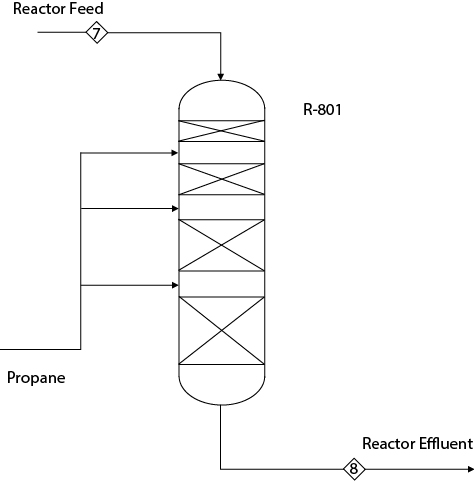
Figure P18.1 Alternative Configuration for Cumene Reactor from Problem 18.1

1. Use the exit temperature from a given bed to adjust the amount of diluent fed to that bed.

2. Use the exit temperature from the previous bed to adjust the amount of diluent fed to the next bed.

3. To what types of control strategy do Parts (a) and (b) conform? Which scheme do you think is better for this type of reactor? Explain your reasoning.

4. Devise a control strategy that incorporates both the ideas used in Parts (a) and (b).

2. Consider the benzene purification column, T-101, in Figure 1.5 for the toluene hydrodealkylation process. The column feed contains noncondensables, mainly methane and a small amount of hydrogen, that must be vented from the system. The vent is taken off the top of the reflux drum, V-104. Sketch a control system in which the valve on this vent line is used to control the pressure of the column. Explain what happens when

1. The column pressure begins to drop

2. The amount of noncondensables fed to the column suddenly increases

3. It has been proposed that the feed toluene to the process shown in Figure 1.5 be vaporized prior to mixing with the hydrogen. It is believed that this scheme will allow more flexibility in the operation of the plant. You have been asked to devise a conceptual design for this vaporizer. The source of heat is the condensation of high-pressure steam. The system designed should be capable of controlling the amount of toluene vaporized and the pressure at which the toluene leaves the vaporizer. Sketch a diagram showing the major pieces of equipment and major control loops.

4. In the DME process shown in Figure B.1.1, the reactor feed exchanges heat with the reactor effluent stream in exchanger E-202. From the diagram, it is evident that the temperature of the stream entering the reactor is controlled by regulating the amount of reactor effluent that is bypassed around the heat exchanger. For this system, answer the following questions:

1. Explain how this system works. For example, explain what happens if the temperature of the feed into E-202 (Stream 4) were to increase or decrease.

2. How would this system respond to fouling in the heat exchanger or a loss of activity of catalyst in the reactor?

3. What type of control strategy is used in this example—feedback, feed-forward, and so on?

4. Design a control system that would regulate the exit temperature of the reactor (Stream 6) rather than the inlet stream temperature.

5. For the benzene column (T-101) in Figure 1.5, do the following:

1. Implement a control scheme that will regulate the purity of the benzene product (Stream 15). You may assume that the purity of this stream can be evaluated by an on-line refractive index monitor placed on Stream 15.

2. What is the type of control system that you have designed in Part (a) called?

6. Consider the feed section of the phthalic anhydride process in Appendix C, Figure C.5. A single control valve is used to control the flow of the combined vaporized naphthalene and air streams, Stream 7. In this process it is important to regulate both the flowrate of Stream 7 and the relative amounts of air and naphthalene in Stream 7. Does the current control scheme allow this type of regulation to occur? If not, devise a control scheme that will allow both these variables to be controlled independently.

7. Describe which form of control strategy (feed-forward, feedback, cascade, or a combination of these) best describes how a responsible person drives an automobile. What would be the consequence of using a feedback control strategy alone?

8. Figure P18.8 shows a CSTR, R-901, carrying out a liquid-phase exothermic reaction. The feed, Stream 1, comes from an upstream unit, and its flowrate is known to vary. The heat of reaction is removed by circulating a portion of the contents of the reactor through an external heat exchanger. Cooling water is used as the cooling utility in E-901.

Figure P18.8 CSTR Configuration for Problem 18.8

For this reactor scheme, devise a system to implement the following control actions:

1. Regulate the temperature of the reactor

2. Regulate the inventory of the reactor, that is, keep a constant liquid level

Explain how your control system would compensate for a change in the flowrate of Stream 1.

What additional control scheme would be needed to maintain a constant conversion in the reactor, assuming that constant conversion can be achieved by ensuring constant residence time in the reactor?

9. Figure P18.9 shows a CSTR carrying out a liquid-phase, exothermic reaction. The heat released partially vaporizes the contents of the reactor. This vapor is condensed in an external condenser, and the condensate is returned to the reactor. The reactor operates at the boiling point (T and P) of the mixture in the CSTR. The vapor formed consists of reactants and products.

Figure P18.9 CSTR Configuration for Problem 18.9

For this system, devise a system to regulate the following variables:

1. Temperature in reactor

2. Residence time in the reactor

Explain how your system would respond to the following changes:

1. Increase in flowrate of feed

2. Fouling of the tubes (on cw side) of the condenser

10. Consider the feed section of the toluene process given in Figure 1.5. The flow of fresh toluene, Stream 1, is regulated by monitoring the level in the toluene storage tank, V-101. If the level is seen to drop, then the valve on Stream 1 opens and vice versa. This is an example of a feedback material balance control loop. For this system, implement a feed-forward control scheme in which the flow of the recycle, Stream 11, is measured and used to control the flow of Stream 1. Do you foresee any potential problems with this control strategy?

11. In the feed section of the maleic anhydride process shown in Figure B.5.1, consider that the air flowrate must be regulated so that a desired ratio between benzene and air is maintained. However, as the air flow changes, the discharge pressure of C-601 should also be maintained at a desired set point. Devise a control scheme to achieve the desired regulation. What type of control system did you design? Why?

12. In the maleic anhydride process shown in Figure B.5.1, the temperature of Stream 6 at the outlet of the feed heater, H-601, needs to be maintained. For this system, do the following:

1. Devise a control scheme for maintaining the temperature of Stream 6 by manipulating the flowrate of the natural gas to the furnace (i.e., firing rate of H-601). The flowrate of combustion air must be maintained at a desired ratio to the flowrate of the natural gas.

2. In an alternative scenario, it is decided that, for maintaining the furnace temperature, fuel oil will be used to minimize the consumption of natural gas. When the fuel oil alone is not sufficient to maintain the temperature, natural gas will be fired along with the fuel oil. The flowrate of combustion air should be regulated such that the desired ratios with respect to the flowrate of the natural gas and the fuel oil are both maintained. Devise a control scheme to achieve this control objective. What type of control system(s) did you design? As the fuel oil and the natural gas have very different heating values, what challenge would you expect in achieving a satisfactory performance with this control scheme?

13. In Example 18.10, there are two switches to start the pump. In addition, consider that the pump can be automatically started by a newly installed high-level switch as long as the stop switches are not pressed. Modify the ladder diagram shown in Figure E18.10(b) accordingly.

14. Consider Problem 18.13. The control logic is now modified such that the pump can be automatically started by the high-level switch even though the stop switches are pressed. Modify the ladder diagram you developed in Problem 18.13 accordingly.

15. In the distillation column shown in Figure 18.10, changes in the feed composition give rise to noncondensables in the tower overhead vapor. Devise a new control scheme for the tower top pressure. It is also desired that instead of controlling the composition of the tower top product, the tower top temperature is controlled as a surrogate control obejective. Modify the existing control scheme accordingly.