

Statistical Intervals for a Single Sample

Chapter Outline
8-1 Confidence Interval on the Mean of a Normal Distribution, Variance Known
8-1.1 Development of the Confidence Interval and Its Basic Properties
8-1.3 One-Sided Confidence Bounds
8-1.4 General Method to Derive a Confidence Interval
8-1.5 Large-Sample Confidence Interval for μ
8-2 Confidence Interval on the Mean of a Normal Distribution, Variance Unknown
8-2.2 Confidence Interval on μ
8-3 Confidence Interval on the Variance And Standard Deviation of a Normal Distribution
8-4 Large-Sample Confidence Interval for a Population Proportion
8-5 Guidelines for Constructing Confidence Intervals
8-6 Bootstrap Confidence Interval
8-7 Tolerance and Prediction intervals
Introduction
Engineers are often involved in estimating parameters. For example, there is an ASTM Standard E23 that defines a technique called the Charpy V-notch method for notched bar impact testing of metallic materials. The impact energy is often used to determine whether the material experiences a ductile-to-brittle transition as the temperature decreases. Suppose that we have tested a sample of 10 specimens of a particular material with this procedure. We know that we can use the sample average ![]() to estimate the true mean impact energy μ. However, we also know that the true mean impact energy is unlikely to be exactly equal to your estimate. Reporting the results of your test as a single number is unappealing because nothing inherent in
to estimate the true mean impact energy μ. However, we also know that the true mean impact energy is unlikely to be exactly equal to your estimate. Reporting the results of your test as a single number is unappealing because nothing inherent in ![]() provides any information about how close it is to μ. Our estimate could be very close, or it could be considerably far from the true mean. A way to avoid this is to report the estimate in terms of a range of plausible values called a confidence interval. A confidence interval always specifies a confidence level, usually 90%, 95%, or 99%, which is a measure of the reliability of the procedure. So if a 95% confidence interval on the impact energy based on the data from our 10 specimens has a lower limit of 63.84J and an upper limit of 65.08J, then we can say that at the 95% level of confidence any value of mean impact energy between 63.84J and 65.08J is a plausible value. By reliability, we mean that if we repeated this experiment over and over again, 95% of all samples would produce a confidence interval that contains the true mean impact energy, and only 5% of the time would the interval be in error. In this chapter, you will learn how to construct confidence intervals and other useful types of statistical intervals for many important types of problem situations.
provides any information about how close it is to μ. Our estimate could be very close, or it could be considerably far from the true mean. A way to avoid this is to report the estimate in terms of a range of plausible values called a confidence interval. A confidence interval always specifies a confidence level, usually 90%, 95%, or 99%, which is a measure of the reliability of the procedure. So if a 95% confidence interval on the impact energy based on the data from our 10 specimens has a lower limit of 63.84J and an upper limit of 65.08J, then we can say that at the 95% level of confidence any value of mean impact energy between 63.84J and 65.08J is a plausible value. By reliability, we mean that if we repeated this experiment over and over again, 95% of all samples would produce a confidence interval that contains the true mean impact energy, and only 5% of the time would the interval be in error. In this chapter, you will learn how to construct confidence intervals and other useful types of statistical intervals for many important types of problem situations.
![]() Learning Objectives
Learning Objectives
After careful study of this chapter, you should be able to do the following:
- Construct confidence intervals on the mean of a normal distribution, using either the normal distribution or the t distribution method
- Construct confidence intervals on the variance and standard deviation of a normal distribution
- Construct confidence intervals on a population proportion
- Use a general method for constructing an approximate confidence interval on a parameter
- Construct prediction intervals for a future observation
- Construct a tolerance interval for a normal population
- Explain the three types of interval estimates: confidence intervals, prediction intervals, and tolerance intervals
In the previous chapter, we illustrated how a point estimate of a parameter can be estimated from sample data. However, it is important to understand how good the estimate obtained is. For example, suppose that we estimate the mean viscosity of a chemical product to be ![]() =
= ![]() = 1000. Now because of sampling variability, it is almost never the case that the true mean μ is exactly equal to the estimate
= 1000. Now because of sampling variability, it is almost never the case that the true mean μ is exactly equal to the estimate ![]() . The point estimate says nothing about how close
. The point estimate says nothing about how close ![]() is to μ. Is the process mean likely to be between 900 and 1100? Or is it likely to be between 990 and 1010? The answer to these questions affects our decisions regarding this process. Bounds that represent an interval of plausible values for a parameter are examples of an interval estimate. Surprisingly, it is easy to determine such intervals in many cases, and the same data that provided the point estimate are typically used.
is to μ. Is the process mean likely to be between 900 and 1100? Or is it likely to be between 990 and 1010? The answer to these questions affects our decisions regarding this process. Bounds that represent an interval of plausible values for a parameter are examples of an interval estimate. Surprisingly, it is easy to determine such intervals in many cases, and the same data that provided the point estimate are typically used.
An interval estimate for a population parameter is called a confidence interval. Information about the precision of estimation is conveyed by the length of the interval. A short interval implies precise estimation. We cannot be certain that the interval contains the true, unknown population parameter—we use only a sample from the full population to compute the point estimate and the interval. However, the confidence interval is constructed so that we have high confidence that it does contain the unknown population parameter. Confidence intervals are widely used in engineering and the sciences.
A tolerance interval is another important type of interval estimate. For example, the chemical product viscosity data might be assumed to be normally distributed. We might like to calculate limits that bound 95% of the viscosity values. For a normal distribution, we know that 95% of the distribution is in the interval
![]()
However, this is not a useful tolerance interval because the parameters μ and σ are unknown. Point estimates such as ![]() and s can be used in the preceding equation for μ and σ. However, we need to account for the potential error in each point estimate to form a tolerance interval for the distribution. The result is an interval of the form
and s can be used in the preceding equation for μ and σ. However, we need to account for the potential error in each point estimate to form a tolerance interval for the distribution. The result is an interval of the form
![]()
where k is an appropriate constant (that is larger than 1.96 to account for the estimation error). As in the case of a confidence interval, it is not certain that the tolerance interval bounds 95% of the distribution, but the interval is constructed so that we have high confidence that it does. Tolerance intervals are widely used and, as we will subsequently see, they are easy to calculate for normal distributions.
Confidence and tolerance intervals bound unknown elements of a distribution. In this chapter, you will learn to appreciate the value of these intervals. A prediction interval provides bounds on one (or more) future observations from the population. For example, a prediction interval could be used to bound a single, new measurement of viscosity—another useful interval. With a large sample size, the prediction interval for normally distributed data tends to the tolerance interval, but for more modest sample sizes, the prediction and tolerance intervals are different.
Keep the purpose of the three types of interval estimates clear:
- A confidence interval bounds population or distribution parameters (such as the mean viscosity).
- A tolerance interval bounds a selected proportion of a distribution.
- A prediction interval bounds future observations from the population or distribution.
Our experience has been that it is easy to confuse the three types of intervals. For example, a confidence interval is often reported when the problem situation calls for a prediction interval.
8-1 Confidence Interval on the Mean of a Normal Distribution, Variance Known
The basic ideas of a confidence interval (CI) are most easily understood by initially considering a simple situation. Suppose that we have a normal population with unknown mean μ and known variance σ2. This is a somewhat unrealistic scenario because typically both the mean and variance are unknown. However, in subsequent sections, we will present confidence intervals for more general situations.
8-1.1 DEVELOPMENT OF THE CONFIDENCE INTERVAL AND ITS BASIC PROPERTIES
Suppose that X1, X2,..., Xn is a random sample from a normal distribution with unknown mean μ and known variance σ2. From the results of Chapter 5, we know that the sample mean ![]() is normally distributed with mean μ and variance σ2/n. We may standardize
is normally distributed with mean μ and variance σ2/n. We may standardize ![]() by subtracting the mean and dividing by the standard deviation, which results in the variable
by subtracting the mean and dividing by the standard deviation, which results in the variable
![]()
The random variable Z has a standard normal distribution.
A confidence interval estimate for μ is an interval of the form l ≤ μ ≤ u, where the end-points l and u are computed from the sample data. Because different samples will produce different values of l and u, these end-points are values of random variables L and U, respectively. Suppose that we can determine values of L and U such that the following probability statement is true:
![]()
where 0 ≤ α ≤ 1. There is a probability of 1 − α of selecting a sample for which the CI will contain the true value of μ. Once we have selected the sample, so that X1 = x1, X2 = x2,..., Xn = xn, and computed l and u, the resulting confidence interval for μ is
![]()
The end-points or bounds l and u are called the lower- and upper-confidence limits (bounds), respectively, and 1 − α is called the confidence coefficient.
In our problem situation, because Z = ![]() has a standard normal distribution, we may write
has a standard normal distribution, we may write
![]()
Now manipulate the quantities inside the brackets by (1) multiplying through by σ/![]() , (2) subtracting
, (2) subtracting ![]() from each term, and (3) multiplying through by − 1. This results in
from each term, and (3) multiplying through by − 1. This results in
![]()
This is a random interval because the end-points ![]() involve the random variable
involve the random variable ![]() . From consideration of Equation 8-4, the lower and upper end-points or limits of the inequalities in Equation 8-4 are the lower- and upper-confidence limits L and U, respectively. This leads to the following definition.
. From consideration of Equation 8-4, the lower and upper end-points or limits of the inequalities in Equation 8-4 are the lower- and upper-confidence limits L and U, respectively. This leads to the following definition.
Confidence Interval on the Mean, Variance Known
If ![]() is the sample mean of a random sample of size n from a normal population with known variance σ2, a 100(1 − α)% CI on μ is given by
is the sample mean of a random sample of size n from a normal population with known variance σ2, a 100(1 − α)% CI on μ is given by
![]()
where zα/2 is the upper 100α/2 percentage point of the standard normal distribution.
The development of this CI assumed that we are sampling from a normal population. The CI is quite robust to this assumption. That is, moderate departures from normality are of no serious concern. From a practical viewpoint, this implies that an advertised 95% CI might have actual confidence of 93% or 94%.
Example 8-1 Metallic Material Transition ASTM Standard E23 defines standard test methods for notched bar impact testing of metallic materials. The Charpy V-notch (CVN) technique measures impact energy and is often used to determine whether or not a material experiences a ductile-to-brittle transition with decreasing temperature. Ten measurements of impact energy (J) on specimens of A238 steel cut at 60°C are as follows: 64.1, 64.7, 64.5, 64.6, 64.5, 64.3, 64.6, 64.8, 64.2, and 64.3. Assume that impact energy is normally distributed with σ = 1J. We want to find a 95% CI for μ, the mean impact energy. The required quantities are zα/2 = z0.025 = 1.96, n = 10, σ = 1, and ![]() = 64.46. The resulting 95% CI is found from Equation 8-5 as follows:
= 64.46. The resulting 95% CI is found from Equation 8-5 as follows:
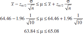
Practical Interpretation: Based on the sample data, a range of highly plausible values for mean impact energy for A238 steel at 60°C is 63.84 J ≤ μ ≤ 65.08 J.
Interpreting a Confidence Interval
How does one interpret a confidence interval? In the impact energy estimation problem in Example 8-1, the 95% CI is 63.84 ≤ μ ≤ 65.08, so it is tempting to conclude that μ is within this interval with probability 0.95. However, with a little reflection, it is easy to see that this cannot be correct; the true value of μ is unknown, and the statement 63.84 ≤ μ ≤ 65.08 is either correct (true with probability 1) or incorrect (false with probability 1). The correct interpretation lies in the realization that a CI is a random interval because in the probability statement defining the end-points of the interval (Equation 8-2), L and U are random variables. Consequently, the correct interpretation of a 100(1 − α)% CI depends on the relative frequency view of probability. Specifically, if an infinite number of random samples are collected and a 100(1 − α)% confidence interval for μ is computed from each sample, 100(1 − α)% of these intervals will contain the true value of μ.
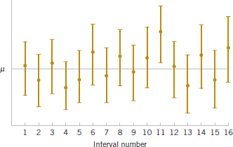
FIGURE 8-1 Repeated construction of a confidence interval for μ.
The situation is illustrated in Fig. 8-1, which shows several 100(1 − α)% confidence intervals for the mean μ of a normal distribution. The dots at the center of the intervals indicate the point estimate of μ (that is, ![]() ). Notice that one of the intervals fails to contain the true value of μ. If this were a 95% confidence interval, in the long run only 5% of the intervals would fail to contain μ.
). Notice that one of the intervals fails to contain the true value of μ. If this were a 95% confidence interval, in the long run only 5% of the intervals would fail to contain μ.
Now in practice, we obtain only one random sample and calculate one confidence interval. Because this interval either will or will not contain the true value of μ, it is not reasonable to attach a probability level to this specific event. The appropriate statement is that the observed interval [l, u] brackets the true value of μ with confidence 100(1 − α). This statement has a frequency interpretation; that is, we do not know whether the statement is true for this specific sample, but the method used to obtain the interval [l, u] yields correct statements 100(1 − α)% of the time.
Confidence Level and Precision of Estimation
Notice that in Example 8-1, our choice of the 95% level of confidence was essentially arbitrary. What would have happened if we had chosen a higher level of confidence, say, 99%? In fact, is it not reasonable that we would want the higher level of confidence? At α = 0.01, we find zα/2 = z0.01/2 = z0.005 = 2.58, while for α = 0.05, z0.025 = 1.96. Thus, the length of the 95% confidence interval is
![]()
whereas the length of the 99% CI is
![]()
Thus, the 99% CI is longer than the 95% CI. This is why we have a higher level of confidence in the 99% confidence interval. Generally, for a fixed sample size n and standard deviation σ, the higher the confidence level, the longer the resulting CI.
The length of a confidence interval is a measure of the precision of estimation. Many authors define the half-length of the CI (in our case zα/2σ/![]() ) as the bound on the error in estimation of the parameter. From the preceeding discussion, we see that precision is inversely related to the confidence level. It is desirable to obtain a confidence interval that is short enough for decision-making purposes and that also has adequate confidence. One way to achieve this is by choosing the sample size n to be large enough to give a CI of specified length or precision with prescribed confidence.
) as the bound on the error in estimation of the parameter. From the preceeding discussion, we see that precision is inversely related to the confidence level. It is desirable to obtain a confidence interval that is short enough for decision-making purposes and that also has adequate confidence. One way to achieve this is by choosing the sample size n to be large enough to give a CI of specified length or precision with prescribed confidence.
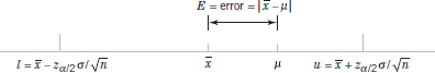
FIGURE 8-2 Error in estimating μ with ![]() .
.
8-1.2 CHOICE OF SAMPLE SIZE
The precision of the confidence interval in Equation 8-5 is 2zα/2σ/![]() . This means that in using
. This means that in using ![]() to estimate μ, the error E = |
to estimate μ, the error E = |![]() − μ| is less than or equal to zα/2σ/
− μ| is less than or equal to zα/2σ/![]() with confidence 100(1 − α). This is shown graphically in Fig. 8-2. In situations whose sample size can be controlled, we can choose n so that we are 100(1 − α)% confident that the error in estimating μ is less than a specified bound on the error E. The appropriate sample size is found by choosing n such that zα/2σ/
with confidence 100(1 − α). This is shown graphically in Fig. 8-2. In situations whose sample size can be controlled, we can choose n so that we are 100(1 − α)% confident that the error in estimating μ is less than a specified bound on the error E. The appropriate sample size is found by choosing n such that zα/2σ/![]() = E. Solving this equation gives the following formula for n.
= E. Solving this equation gives the following formula for n.
Sample Size for Specified Error on the Mean, Variance Known
If ![]() is used as an estimate of μ, we can be 100(1 − α)% confident that the error |
is used as an estimate of μ, we can be 100(1 − α)% confident that the error |![]() − μ| will not exceed a specified amount E when the sample size is
− μ| will not exceed a specified amount E when the sample size is
![]()
If the right-hand side of Equation 8-6 is not an integer, it must be rounded up. This will ensure that the level of confidence does not fall below 100(1 − α)%. Notice that 2E is the length of the resulting confidence interval.
Example 8-2 Metallic Material Transition To illustrate the use of this procedure, consider the CVN test described in Example 8-1 and suppose that we want to determine how many specimens must be tested to ensure that the 95% CI on μ for A238 steel cut at 60°C has a length of at most 1.0J. Because the bound on error in estimation E is one-half of the length of the CI, to determine n, we use Equation 8-6 with E = 0.5, σ = 1, and zα/2 = 1.96. The required sample size is,
![]()
and because n must be an integer, the required sample size is n = 16.
Notice the general relationship between sample size, desired length of the confidence interval 2E, confidence level 100(1 − α), and standard deviation σ:
- As the desired length of the interval 2E decreases, the required sample size n increases for a fixed value of σ and specified confidence.
- As σ increases, the required sample size n increases for a fixed desired length 2E and specified confidence.
- As the level of confidence increases, the required sample size n increases for fixed desired length 2E and standard deviation σ.
8-1.3 ONE-SIDED CONFIDENCE BOUNDS
The confidence interval in Equation 8-5 gives both a lower confidence bound and an upper confidence bound for μ. Thus, it provides a two-sided CI. It is also possible to obtain one-sided confidence bounds for m by setting either the lower bound l = −∞ or the upper bound u = ∞ and replacing zα/2 by zα.
One-Sided Confidence Bounds on the Mean, Variance Known
A 100(1 − α)% upper-confidence bound for μ is
![]()
and a 100(1 − α)% lower-confidence bound for μ is
![]()
Example 8-3 One-Sided Confidence Bound The same data for impact testing from Example 8-1 are used to construct a lower, one-sided 95% confidence interval for the mean impact energy. Recall that ![]() = 64.46, σ = 1J, and n = 10. The interval is
= 64.46, σ = 1J, and n = 10. The interval is
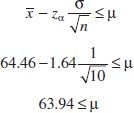
Practical Interpretation: The lower limit for the two-sided interval in Example 8-1 was 63.84. Because zα < zα/2, the lower limit of a one-sided interval is always greater than the lower limit of a two-sided interval of equal confidence. The one-sided interval does not bound μ from above so that it still achieves 95% confidence with a slightly larger lower limit. If our interest is only in the lower limit for μ, then the one-sided interval is preferred because it provides equal confidence with a greater limit. Similarly, a one-sided upper limit is always less than a two-sided upper limit of equal confidence.
8-1.4 GENERAL METHOD TO DERIVE A CONFIDENCE INTERVAL
It is easy to give a general method for finding a confidence interval for an unknown parameter θ. Let X1, X2,..., Xn be a random sample of n observations. Suppose that we can find a statistic g(X1, X2,..., Xn; θ) with the following properties:
- g(X1, X2,..., Xn; θ) depends on both the sample and θ.
- The probability distribution of g(X1, X2,..., Xn; θ) does not depend on θ or any other unknown parameter.
In the case considered in this section, the parameter θ = μ. The random variable g(X1, X2,..., Xn; μ) = (![]() − μ)/(σ/
− μ)/(σ/![]() ) satisfies both conditions; the random variable depends on the sample and on μ, and it has a standard normal distribution because σ is known. Now we must find constants CL and CU so that
) satisfies both conditions; the random variable depends on the sample and on μ, and it has a standard normal distribution because σ is known. Now we must find constants CL and CU so that
![]()
Because of property 2, CL and CU do not depend on θ. In our example, CL = −zα/2 and CU = zα/2. Finally, we must manipulate the inequalities in the probability statement so that
![]()
This gives L(X1, X2,..., Xn) and U(X1, X2,..., Xn) as the lower and upper confidence limits defining the 100(1 − α) confidence interval for θ. The quantity g(X1, X2,..., Xn; θ) is often called a pivotal quantity because we pivot on this quantity in Equation 8-9 to produce Equation 8-10. In our example, we manipulated the pivotal quantity (![]() − μ)/(σ/
− μ)/(σ/![]() ) to obtain L(X1, X2,... Xn) =
) to obtain L(X1, X2,... Xn) = ![]() − zα/2σ/
− zα/2σ/![]() and U(X1, X2,..., Xn) =
and U(X1, X2,..., Xn) = ![]() + zα/2σ/
+ zα/2σ/![]() .
.
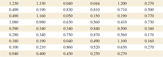
Example 8-4 The Exponential Distribution The exponential distribution is used extensively in the fields of reliability engineering and communications technology because it has been shown to be an excellent model for many of the kinds of problems encountered. For example, the call-handling (processing) time in telephone networks often follows an exponential distribution. A sample of n = 10 calls had the following durations (in minutes):
![]()
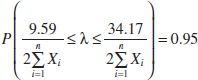
Assume that call-handling time is exponentially distributed. Find a 95% two-sided CI on both the parameter λ of the exponential distribution and the mean call-handling time.
If X is an exponential random variable, it can be shown that 2λ![]() Xi is a chi-square distributed random variable with 2n degrees of freedom (the chi-square distribution will be formally introduced in Section 8.3). So we can let g(x1,x2,...xn;θ) in Equation (8-9) equal
Xi is a chi-square distributed random variable with 2n degrees of freedom (the chi-square distribution will be formally introduced in Section 8.3). So we can let g(x1,x2,...xn;θ) in Equation (8-9) equal ![]() Xi and let CL and CU in that equation be the lower-tailed and upper-tailed 2½ percentage points of the chi-square distribution, which are given in Appendix Table IV. For 2n = 2(10) = 20 degrees of freedom, these percentage points are CL = 9.59 and CU = 34.17, respectively. Therefore, Equation (8-9) becomes
Xi and let CL and CU in that equation be the lower-tailed and upper-tailed 2½ percentage points of the chi-square distribution, which are given in Appendix Table IV. For 2n = 2(10) = 20 degrees of freedom, these percentage points are CL = 9.59 and CU = 34.17, respectively. Therefore, Equation (8-9) becomes
![]()
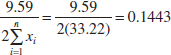
Rearranging the quantities inside the probability statement by dividing through by ![]() Xi gives
Xi gives
From the sample data, we find that ![]() = 33.22, so the lower confidence bound on λ is
= 33.22, so the lower confidence bound on λ is
and the upper confidence bound is
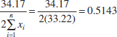
The 95% two-sided CI on λ is
![]()
The 95% confidence interval on the mean call-handling time is found using the relationship between the mean μ of the exponential distribution and the parameter λ; that is, μ = 1/λ. The resulting 95% CI on μ is 1/0.5143 ≤ μ = 1/λ ≤ 1/0.1443, or
![]()
Therefore, we are 95% confident that the mean call-handling time in this telephone network is between 1.9444 and 6.9300 minutes.
8-1.5 LARGE-SAMPLE CONFIDENCE INTERVAL FOR μ
We have assumed that the population distribution is normal with unknown mean and known standard deviation σ. We now present a large-sample CI for μ that does not require these assumptions. Let X1, X2,..., Xn be a random sample from a population with unknown mean μ and variance σ2. Now if the sample size n is large, the central limit theorem implies that ![]() has approximately a normal distribution with mean μ and variance σ2/n. Therefore, Z = (
has approximately a normal distribution with mean μ and variance σ2/n. Therefore, Z = (![]() − μ)/(σ/
− μ)/(σ/![]() ) has approximately a standard normal distribution. This ratio could be used as a pivotal quantity and manipulated as in Section 8-1.1 to produce an approximate CI for μ. However, the standard deviation σ is unknown. It turns out that when n is large, replacing σ by the sample standard deviation S has little effect on the distribution of Z. This leads to the following useful result.
) has approximately a standard normal distribution. This ratio could be used as a pivotal quantity and manipulated as in Section 8-1.1 to produce an approximate CI for μ. However, the standard deviation σ is unknown. It turns out that when n is large, replacing σ by the sample standard deviation S has little effect on the distribution of Z. This leads to the following useful result.
Large-Sample Confidence Interval on the Mean
When n is large, the quantity
![]()
has an approximate standard normal distribution. Consequently,
![]()
is a large-sample confidence interval for μ, with confidence level of approximately 100(1 − α)%.
Equation 8-11 holds regardless of the shape of the population distribution. Generally, n should be at least 40 to use this result reliably. The central limit theorem generally holds for n ≥ 30, but the larger sample size is recommended here because replacing s with S in Z results in additional variability.
Example 8-5 Mercury Contamination An article in the 1993 volume of the Transactions of the American Fisheries Society reports the results of a study to investigate the mercury contamination in large-mouth bass. A sample of fish was selected from 53 Florida lakes, and mercury concentration in the muscle tissue was measured (ppm). The mercury concentration values were
The summary statistics for these data are as follows:
![]()
Figure 8-3 presents the histogram and normal probability plot of the mercury concentration data. Both plots indicate that the distribution of mercury concentration is not normal and is positively skewed. We want to find an approximate 95% CI on μ. Because n > 40, the assumption of normality is not necessary to use in Equation 8-11. The required quantities are n = 53, ![]() = 0.5250, s = 0.3486, and z0.025 = 1.96. The approximate 95% CI on μ is
= 0.5250, s = 0.3486, and z0.025 = 1.96. The approximate 95% CI on μ is
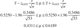
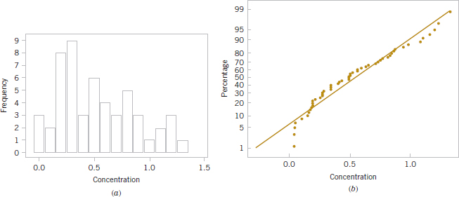
FIGURE 8-3 Mercury concentration in largemouth bass. (a) Histogram. (b) Normal probability plot.
Practical Interpretation: This interval is fairly wide because there is substantial variability in the mercury concentration measurements. A larger sample size would have produced a shorter interval.
Large-Sample Confidence Interval for a Parameter
The large-sample confidence interval for μ in Equation 8-11 is a special case of a more general result. Suppose that θ is a parameter of a probability distribution, and let ![]() be an estimator of θ. If
be an estimator of θ. If ![]() (1) has an approximate normal distribution, (2) is approximately unbiased for θ, and (3) has standard deviation
(1) has an approximate normal distribution, (2) is approximately unbiased for θ, and (3) has standard deviation ![]() that can be estimated from the sample data, the quantity (
that can be estimated from the sample data, the quantity (![]() − 0)/
− 0)/![]() has an approximate standard normal distribution. Then a large-sample approximate CI for θ is given by
has an approximate standard normal distribution. Then a large-sample approximate CI for θ is given by
Large-Sample Approximate Confidence Interval
![]()
Maximum likelihood estimators usually satisfy the three conditions just listed, so Equation 8-12 is often used when ![]() is the maximum likelihood estimator of θ. Finally, note that Equation 8-12 can be used even when
is the maximum likelihood estimator of θ. Finally, note that Equation 8-12 can be used even when ![]() is a function of other unknown parameters (or of θ). Essentially, we simply use the sample data to compute estimates of the unknown parameters and substitute those estimates into the expression for
is a function of other unknown parameters (or of θ). Essentially, we simply use the sample data to compute estimates of the unknown parameters and substitute those estimates into the expression for ![]() .
.
![]() Problem available in WileyPLUS at instructor's discretion.
Problem available in WileyPLUS at instructor's discretion.
![]() Go Tutorial Tutoring problem available in WileyPLUS at instructor's discretion
Go Tutorial Tutoring problem available in WileyPLUS at instructor's discretion
8-1. ![]() For a normal population with known variance σ2, answer the following questions:
For a normal population with known variance σ2, answer the following questions:
(a) What is the confidence level for the interval ![]() − 2.14σ/
− 2.14σ/![]() ≤ μ ≤
≤ μ ≤ ![]() + 2.14σ/
+ 2.14σ/![]() ?
?
(b) What is the confidence level for the interval ![]() − 2.49σ/
− 2.49σ/![]()
![]() − 2.49σ/
− 2.49σ/![]() ≤ μ ≤
≤ μ ≤ ![]() + 2.49σ/
+ 2.49σ/![]() ?
?
(c) What is the confidence level for the interval ![]() − 1.85σ/
− 1.85σ/![]() ≤ μ ≤
≤ μ ≤ ![]() + 1.85σ/
+ 1.85σ/![]() ?
?
(d) What is the confidence level for the interval μ ≤ ![]() + 2.00σ/
+ 2.00σ/![]() ?
?
(e) What is the confidence level for the interval ![]() − 1.96σ/
− 1.96σ/![]() ≤ μ?
≤ μ?
8-2. For a normal population with known variance σ2:
(a) What value of zα/2 in Equation 8-5 gives 98% confidence?
(b) What value of zα/2 in Equation 8-5 gives 80% confidence?
(c) What value of zα/2 in Equation 8-5 gives 75% confidence?
8-3. ![]() Consider the one-sided confidence interval expressions for a mean of a normal population.
Consider the one-sided confidence interval expressions for a mean of a normal population.
(a) What value of zα would result in a 90% CI?
(b) What value of zα would result in a 95% CI?
(c) What value of zα would result in a 99% CI?
8-4. ![]() A confidence interval estimate is desired for the gain in a circuit on a semiconductor device. Assume that gain is normally distributed with standard deviation s = 20.
A confidence interval estimate is desired for the gain in a circuit on a semiconductor device. Assume that gain is normally distributed with standard deviation s = 20.
(a) Find a 95% CI for m when n = 10 and ![]() = 1000.
= 1000.
(b) Find a 95% CI for m when n = 25 and ![]() = 1000.
= 1000.
(c) Find a 99% CI for m when n = 10 and ![]() = 1000.
= 1000.
(d) Find a 99% CI for m when n = 25 and ![]() = 1000.
= 1000.
(e) How does the length of the CIs computed change with the changes in sample size and confidence level?
8-5. A random sample has been taken from a normal distribution and the following confidence intervals constructed using the same data: (38.02, 61.98) and (39.95, 60.05)
(a) What is the value of the sample mean?
(b) One of these intervals is a 95% CI and the other is a 90% CI. Which one is the 95% CI and why?
8-6. A random sample has been taken from a normal distribution and the following confidence intervals constructed using the same data: (37.53, 49.87) and (35.59, 51.81)
(a) What is the value of the sample mean?
(b) One of these intervals is a 99% CI and the other is a 95% CI. Which one is the 95% CI and why?
8-7. ![]() Consider the gain estimation problem in Exercise 8-4.
Consider the gain estimation problem in Exercise 8-4.
(a) How large must n be if the length of the 95% CI is to be 40?
(b) How large must n be if the length of the 99% CI is to be 40?
8-8. Following are two confidence interval estimates of the mean m of the cycles to failure of an automotive door latch mechanism (the test was conducted at an elevated stress level to accelerate the failure).
![]()
(a) What is the value of the sample mean cycles to failure?
(b) The confidence level for one of these CIs is 95% and for the other is 99%. Both CIs are calculated from the same sample data. Which is the 95% CI? Explain why.
8-9. Suppose that n = 100 random samples of water from a freshwater lake were taken and the calcium concentration (milligrams per liter) measured. A 95% CI on the mean calcium concentration is 0.49 ≤ μ ≤ 0.82.
(a) Would a 99% CI calculated from the same sample data be longer or shorter?
(b) Consider the following statement: There is a 95% chance that μ is between 0.49 and 0.82. Is this statement correct? Explain your answer.
(c) Consider the following statement: If n = 100 random samples of water from the lake were taken and the 95% CI on μ computed, and this process were repeated 1000 times, 950 of the CIs would contain the true value of μ. Is this statement correct? Explain your answer.
8-10. ![]() Past experience has indicated that the breaking strength of yarn used in manufacturing drapery material is normally distributed and that σ = 2 psi. A random sample of nine specimens is tested, and the average breaking strength is found to be 98 psi. Find a 95% two-sided confidence interval on the true mean breaking strength.
Past experience has indicated that the breaking strength of yarn used in manufacturing drapery material is normally distributed and that σ = 2 psi. A random sample of nine specimens is tested, and the average breaking strength is found to be 98 psi. Find a 95% two-sided confidence interval on the true mean breaking strength.
8-11. ![]() The yield of a chemical process is being studied. From previous experience, yield is known to be normally distributed and σ = 3. The past five days of plant operation have resulted in the following percent yields: 91.6, 88.75, 90.8, 89.95, and 91.3. Find a 95% two-sided confidence interval on the true mean yield.
The yield of a chemical process is being studied. From previous experience, yield is known to be normally distributed and σ = 3. The past five days of plant operation have resulted in the following percent yields: 91.6, 88.75, 90.8, 89.95, and 91.3. Find a 95% two-sided confidence interval on the true mean yield.
8-12. ![]() The diameter of holes for a cable harness is known to have a normal distribution with σ = 0.01 inch. A random sample of size 10 yields an average diameter of 1.5045 inch. Find a 99% two-sided confidence interval on the mean hole diameter.
The diameter of holes for a cable harness is known to have a normal distribution with σ = 0.01 inch. A random sample of size 10 yields an average diameter of 1.5045 inch. Find a 99% two-sided confidence interval on the mean hole diameter.
8-13. ![]() A manufacturer produces piston rings for an automobile engine. It is known that ring diameter is normally distributed with σ = 0.001 millimeters. A random sample of 15 rings has a mean diameter of
A manufacturer produces piston rings for an automobile engine. It is known that ring diameter is normally distributed with σ = 0.001 millimeters. A random sample of 15 rings has a mean diameter of ![]() = 74.036 millimeters.
= 74.036 millimeters.
(a) Construct a 99% two-sided confidence interval on the mean piston ring diameter.
(b) Construct a 99% lower-confidence bound on the mean piston ring diameter. Compare the lower bound of this confidence interval with the one in part (a).
8-14. The life in hours of a 75-watt light bulb is known to be normally distributed with σ = 25 hours. A random sample of 20 bulbs has a mean life of ![]() = 1014 hours.
= 1014 hours.
(a) Construct a 95% two-sided confidence interval on the mean life.
(b) Construct a 95% lower-confidence bound on the mean life. Compare the lower bound of this confidence interval with the one in part (a).
8-15. ![]() A civil engineer is analyzing the compressive strength of concrete. Compressive strength is normally distributed with σ2 = 1000(psi)2. A random sample of 12 specimens has a mean compressive strength of
A civil engineer is analyzing the compressive strength of concrete. Compressive strength is normally distributed with σ2 = 1000(psi)2. A random sample of 12 specimens has a mean compressive strength of ![]() = 3250 psi.
= 3250 psi.
(a) Construct a 95% two-sided confidence interval on mean compressive strength.
(b) Construct a 99% two-sided confidence interval on mean compressive strength. Compare the width of this confidence interval with the width of the one found in part (a).
8-16. ![]() Suppose that in Exercise 8-14 we wanted the error in estimating the mean life from the two-sided confidence interval to be five hours at 95% confidence. What sample size should be used?
Suppose that in Exercise 8-14 we wanted the error in estimating the mean life from the two-sided confidence interval to be five hours at 95% confidence. What sample size should be used?
8-17. ![]() Suppose that in Exercise 8-14 you wanted the total width of the two-sided confidence interval on mean life to be six hours at 95% confidence. What sample size should be used?
Suppose that in Exercise 8-14 you wanted the total width of the two-sided confidence interval on mean life to be six hours at 95% confidence. What sample size should be used?
8-18. ![]() Suppose that in Exercise 8-15 it is desired to estimate the compressive strength with an error that is less than 15 psi at 99% confidence. What sample size is required?
Suppose that in Exercise 8-15 it is desired to estimate the compressive strength with an error that is less than 15 psi at 99% confidence. What sample size is required?
8-19. ![]() By how much must the sample size n be increased if the length of the CI on μ in Equation 8-5 is to be halved?
By how much must the sample size n be increased if the length of the CI on μ in Equation 8-5 is to be halved?
8-20. If the sample size n is doubled, by how much is the length of the CI on μ in Equation 8-5 reduced? What happens to the length of the interval if the sample size is increased by a factor of four?
8-21. ![]() Go Tutorial An article in the Journal of Agricultural Science [“The Use of Residual Maximum Likelihood to Model Grain Quality Characteristics of Wheat with Variety, Climatic and Nitrogen Fertilizer Effects” (1997, Vol. 128, pp. 135–142)] investigated means of wheat grain crude protein content (CP) and Hagberg falling number (HFN) surveyed in the United Kingdom. The analysis used a variety of nitrogen fertilizer applications (kg N/ha), temperature (°C), and total monthly rainfall (mm). The following data below describe temperatures for wheat grown at Harper Adams Agricultural College between 1982 and 1993. The temperatures measured in June were obtained as follows:
Go Tutorial An article in the Journal of Agricultural Science [“The Use of Residual Maximum Likelihood to Model Grain Quality Characteristics of Wheat with Variety, Climatic and Nitrogen Fertilizer Effects” (1997, Vol. 128, pp. 135–142)] investigated means of wheat grain crude protein content (CP) and Hagberg falling number (HFN) surveyed in the United Kingdom. The analysis used a variety of nitrogen fertilizer applications (kg N/ha), temperature (°C), and total monthly rainfall (mm). The following data below describe temperatures for wheat grown at Harper Adams Agricultural College between 1982 and 1993. The temperatures measured in June were obtained as follows:
![]()
Assume that the standard deviation is known to be σ = 0.5.
(a) Construct a 99% two-sided confidence interval on the mean temperature.
(b) Construct a 95% lower-confidence bound on the mean temperature.
(c) Suppose that you wanted to be 95% confident that the error in estimating the mean temperature is less than 2 degrees Celsius. What sample size should be used?
(d) Suppose that you wanted the total width of the two-sided confidence interval on mean temperature to be 1.5 degrees Celsius at 95% confidence. What sample size should be used?
8-22. Ishikawa et al. (Journal of Bioscience and Bioengineering, 2012) studied the adhesion of various biofilms to solid surfaces for possible use in environmental technologies. Adhesion assay is conducted by measuring absorbance at A590. Suppose that for the bacterial strain Acinetobacter, five measurements gave readings of 2.69, 5.76, 2.67, 1.62 and 4.12 dyne-cm2. Assume that the standard deviation is known to be 0.66 dyne-cm2.
(a) Find a 95% confidence interval for the mean adhesion.
(b) If the scientists want the confidence interval to be no wider than 0.55 dyne-cm2, how many observations should they take?
8-23. Dairy cows at large commercial farms often receive injections of bST (Bovine Somatotropin), a hormone used to spur milk production. Bauman et al. (Journal of Dairy Science, 1989) reported that 12 cows given bST produced an average of 28.0 kg/d of milk. Assume that the standard deviation of milk production is 2.25 kg/d.
(a) Find a 99% confidence interval for the true mean milk production.
(b) If the farms want the confidence interval to be no wider than ±1.25 kg/d, what level of confidence would they need to use?
8-2 Confidence Interval on the Mean of a Normal Distribution, Variance Unknown
When we are constructing confidence intervals on the mean μ of a normal population when σ2 is known, we can use the procedure in Section 8-1.1. This CI is also approximately valid (because of the central limit theorem) regardless of whether or not the underlying population is normal so long as n is reasonably large (n ≥ 40, say). As noted in Section 8-1.5, we can even handle the case of unknown variance for the large-sample-size situation. However, when the sample is small and σ2 is unknown, we must make an assumption about the form of the underlying distribution to obtain a valid CI procedure. A reasonable assumption in many cases is that the underlying distribution is normal.
Many populations encountered in practice are well approximated by the normal distribution, so this assumption will lead to confidence interval procedures of wide applicability. In fact, moderate departure from normality will have little effect on validity. When the assumption is unreasonable, an alternative is to use nonparametric statistical procedures that are valid for any underlying distribution.
Suppose that the population of interest has a normal distribution with unknown mean μ and unknown variance σ2. Assume that a random sample of size n, say, X1, X2, ..., Xn, is available, and let ![]() and S2 be the sample mean and variance, respectively.
and S2 be the sample mean and variance, respectively.
We wish to construct a two-sided CI on μ. If the variance σ2 is known, we know that Z = (![]() − μ)/(σ/
− μ)/(σ/![]() ) has a standard normal distribution. When σ2 is unknown, a logical procedure is to replace σ with the sample standard deviation S. The random variable Z now becomes T = (
) has a standard normal distribution. When σ2 is unknown, a logical procedure is to replace σ with the sample standard deviation S. The random variable Z now becomes T = (![]() − μ)/(S/
− μ)/(S/![]() ). A logical question is what effect replacing σ with S has on the distribution of the random variable T. If n is large, the answer to this question is “very little,” and we can proceed to use the confidence interval based on the normal distribution from Section 8-1.5. However, n is usually small in most engineering problems, and in this situation, a different distribution must be employed to construct the CI.
). A logical question is what effect replacing σ with S has on the distribution of the random variable T. If n is large, the answer to this question is “very little,” and we can proceed to use the confidence interval based on the normal distribution from Section 8-1.5. However, n is usually small in most engineering problems, and in this situation, a different distribution must be employed to construct the CI.
8-2.1 t DISTRIBUTION
t Distribution
Let X1, X2,..., Xn be a random sample from a normal distribution with unknown mean μ and unknown variance σ2. The random variable
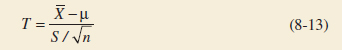
has a t distribution with n − 1 degrees of freedom.
The t probability density function is
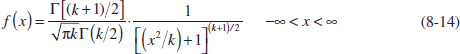
where k is the number of degrees of freedom. The mean and variance of the t distribution are zero and k/(k − 2) (for k > 2), respectively.
Several t distributions are shown in Fig. 8-4. The general appearance of the t distribution is similar to the standard normal distribution in that both distributions are symmetric and unimodal, and the maximum ordinate value is reached when the mean μ = 0. However, the t distribution has heavier tails than the normal; that is, it has more probability in the tails than does the normal distribution. As the number of degrees of freedom k → ∞, the limiting form of the t distribution is the standard normal distribution. Generally, the number of degrees of freedom for t is the number of degrees of freedom associated with the estimated standard deviation.
Appendix Table V provides percentage points of the t distribution. We will let tα,k be the value of the random variable T with k degrees of freedom above which we find an area (or probability) α. Thus, tα,k is an upper-tailed 100α percentage point of the t distribution with k degrees of freedom. This percentage point is shown in Fig. 8-5. In the Appendix Table V, the α values are the column headings, and the degrees of freedom are listed in the left column. To illustrate the use of the table, note that the t-value with 10 degrees of freedom having an area of 0.05 to the right is t0.05,10 = 1.812. That is,
![]()
Because the t distribution is symmetric about zero, we have t1−α,n = −tα,n; that is, the t-value having an area of 1 − α to the right (and therefore an area of a to the left) is equal to the negative of the t-value that has area a in the right tail of the distribution. Therefore, t0.95,10 = −t0.05,10 = −1.812. Finally, because tα,∞ is the standard normal distribution, the familiar zα values appear in the last row of Appendix Table V.
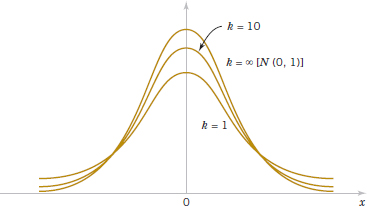
FIGURE 8-4 Probability density functions of several t distributions.
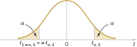
FIGURE 8-5 Percentage points of the t distribution.
8-2.2 t CONFIDENCE INTERVAL ON μ
It is easy to find a 100(1 − α)% confidence interval on the mean of a normal distribution with unknown variance by proceeding essentially as we did in Section 8-1.1. We know that the distribution of T = (![]() − μ)/(S/
− μ)/(S/![]() ) is t with n − 1 degrees of freedom. Letting tα/2,n−1 be the upper 100α/2 percentage point of the t distribution with n − 1 degrees of freedom, we may write
) is t with n − 1 degrees of freedom. Letting tα/2,n−1 be the upper 100α/2 percentage point of the t distribution with n − 1 degrees of freedom, we may write
![]()
or
![]()
Rearranging this last equation yields
![]()
This leads to the following definition of the 100(1 − α)% two-sided confidence interval on μ.
Confidence Interval on the Mean, Variance Unknown
If ![]() and s are the mean and standard deviation of a random sample from a normal distribution with unknown variance σ2, a 100(1 − α)% confidence interval on μ is given by
and s are the mean and standard deviation of a random sample from a normal distribution with unknown variance σ2, a 100(1 − α)% confidence interval on μ is given by
![]()
where tα/2,n−1 is the upper 100α/2 percentage point of the t distribution with n − 1 degrees of freedom.
The assumption underlying this CI is that we are sampling from a normal population. However, the t distribution-based CI is relatively insensitive or robust to this assumption. Checking the normality assumption by constructing a normal probability plot of the data is a good general practice. Small to moderate departures from normality are not a cause for concern.
One-sided confidence bounds on the mean of a normal distribution are also of interest and are easy to find. Simply use only the appropriate lower or upper confidence limit from Equation 8-16 and replace tα/2,n−1 by tα,n−1.
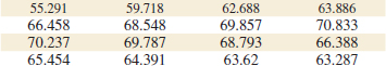
Example 8-6 Alloy Adhesion An article in the journal Materials Engineering (1989, Vol. II, No. 4, pp. 275–281) describes the results of tensile adhesion tests on 22 U-700 alloy specimens. The load at specimen failure is as follows (in megapascals):
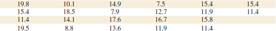
The sample mean is ![]() = 13.71, and the sample standard deviation is s = 3.55. Figures 8-6 and 8-7 show a box plot and a normal probability plot of the tensile adhesion test data, respectively. These displays provide good support for the assumption that the population is normally distributed. We want to find a 95% CI on μ. Since n = 22, we have n − 1 = 21 degrees of freedom for t, so t0.025,21 = 2.080. The resulting CI is
= 13.71, and the sample standard deviation is s = 3.55. Figures 8-6 and 8-7 show a box plot and a normal probability plot of the tensile adhesion test data, respectively. These displays provide good support for the assumption that the population is normally distributed. We want to find a 95% CI on μ. Since n = 22, we have n − 1 = 21 degrees of freedom for t, so t0.025,21 = 2.080. The resulting CI is
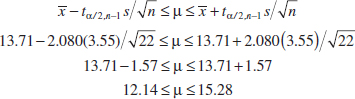
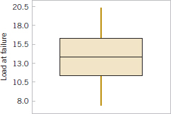
FIGURE 8-6 Box and whisker plot for the load at failure data in Example 8-5.
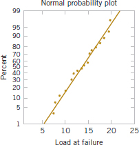
FIGURE 8-7 Normal probability plot of the load at failure data from Example 8-5.
Practical Interpretation: The CI is fairly wide because there is a lot of variability in the tensile adhesion test measurements. A larger sample size would have led to a shorter interval.
It is not as easy to select a sample size n to obtain a specified length (or precision of estimation) for this CI as it was in the known-σ case, because the length of the interval involves s (which is unknown before the data are collected), n, and tα/2,n−1. Note that the t-percentile depends on the sample size n. Consequently, an appropriate n can only be obtained through trial and error. The results of this will, of course, also depend on the reliability of our prior “guess” for σ.
Exercises FOR SECTION 8-2
![]() Problem available in WileyPLUS at instructor's discretion.
Problem available in WileyPLUS at instructor's discretion.
![]() Go Tutorial Tutoring problem available in WileyPLUS at instructor's discretion.
Go Tutorial Tutoring problem available in WileyPLUS at instructor's discretion.
8-24. ![]() Find the values of the following percentiles: t0.025,15, t0.05,10, t0.10,20, t0.005,25, and t0.001,30.
Find the values of the following percentiles: t0.025,15, t0.05,10, t0.10,20, t0.005,25, and t0.001,30.
8-25. ![]() Determine the t-percentile that is required to construct each of the following two-sided confidence intervals:
Determine the t-percentile that is required to construct each of the following two-sided confidence intervals:
(a) Confidence level = 95%, degrees of freedom = 12
(b) Confidence level = 95%, degrees of freedom = 24
(c) Confidence level = 99%, degrees of freedom = 13
(d) Confidence level = 99.9%, degrees of freedom = 15
8-26. ![]() Determine the t-percentile that is required to construct each of the following one-sided confidence intervals:
Determine the t-percentile that is required to construct each of the following one-sided confidence intervals:
(a) Confidence level = 95%, degrees of freedom = 14
(b) Confidence level = 99%, degrees of freedom = 19
(c) Confidence level = 99.9%, degrees of freedom = 24
8-27. A random sample has been taken from a normal distribution. Output from a software package follows:
![]()
(a) Fill in the missing quantities.
(b) Find a 95% CI on the population mean.
8-28. A random sample has been taken from a normal distribution. Output from a software package follows:
![]()
(a) Fill in the missing quantities.
(b) Find a 95% CI on the population mean.
8-29. A research engineer for a tire manufacturer is investigating tire life for a new rubber compound and has built 16 tires and tested them to end-of-life in a road test. The sample mean and standard deviation are 60,139.7 and 3645.94 kilometers. Find a 95% confidence interval on mean tire life.
8-30. ![]() An Izod impact test was performed on 20 specimens of PVC pipe. The sample mean is
An Izod impact test was performed on 20 specimens of PVC pipe. The sample mean is ![]() = 1.25 and the sample standard deviation is s = 0.25. Find a 99% lower confidence bound on Izod impact strength.
= 1.25 and the sample standard deviation is s = 0.25. Find a 99% lower confidence bound on Izod impact strength.
8-31. ![]() A postmix beverage machine is adjusted to release a certain amount of syrup into a chamber where it is mixed with carbonated water. A random sample of 25 beverages was found to have a mean syrup content of
A postmix beverage machine is adjusted to release a certain amount of syrup into a chamber where it is mixed with carbonated water. A random sample of 25 beverages was found to have a mean syrup content of ![]() = 1.10 fluid ounce and a standard deviation of s = 0.015 fluid ounce. Find a 95% CI on the mean volume of syrup dispensed.
= 1.10 fluid ounce and a standard deviation of s = 0.015 fluid ounce. Find a 95% CI on the mean volume of syrup dispensed.
8-32. ![]() An article in Medicine and Science in Sports and Exercise [“Maximal Leg-Strength Training Improves Cycling Economy in Previously Untrained Men” (2005, Vol. 37, pp. 131–136)] studied cycling performance before and after eight weeks of leg-strength training. Seven previously untrained males performed leg-strength training three days per week for eight weeks (with four sets of five replications at 85% of one repetition maximum). Peak power during incremental cycling increased to a mean of 315 watts with a standard deviation of 16 watts. Construct a 95% confidence interval for the mean peak power after training.
An article in Medicine and Science in Sports and Exercise [“Maximal Leg-Strength Training Improves Cycling Economy in Previously Untrained Men” (2005, Vol. 37, pp. 131–136)] studied cycling performance before and after eight weeks of leg-strength training. Seven previously untrained males performed leg-strength training three days per week for eight weeks (with four sets of five replications at 85% of one repetition maximum). Peak power during incremental cycling increased to a mean of 315 watts with a standard deviation of 16 watts. Construct a 95% confidence interval for the mean peak power after training.
8-33. ![]() An article in Obesity Research [“Impaired Pressure Natriuresis in Obese Youths” (2003, Vol. 11, pp. 745–751)] described a study in which all meals were provided for 14 lean boys for three days followed by one stress test (with a video-game task). The average systolic blood pressure (SBP) during the test was 118.3 mm HG with a standard deviation of 9.9 mm HG. Construct a 99% one-sided upper confidence interval for mean SBP.
An article in Obesity Research [“Impaired Pressure Natriuresis in Obese Youths” (2003, Vol. 11, pp. 745–751)] described a study in which all meals were provided for 14 lean boys for three days followed by one stress test (with a video-game task). The average systolic blood pressure (SBP) during the test was 118.3 mm HG with a standard deviation of 9.9 mm HG. Construct a 99% one-sided upper confidence interval for mean SBP.
8-34. An article in the Journal of Composite Materials (December 1989, Vol. 23, p. 1200) describes the effect of delamination on the natural frequency of beams made from composite laminates. Five such delaminated beams were subjected to loads, and the resulting frequencies (in hertz) were as follows:
![]()
Check the assumption of normality in the population. Calculate a 90% two-sided confidence interval on mean natural frequency.
8-35. ![]() The Bureau of Meteorology of the Australian Government provided the mean annual rainfall (in millimeters) in Australia 1983–2002 as follows (http://www.bom.gov.au/climate/change/rain03.txt):
The Bureau of Meteorology of the Australian Government provided the mean annual rainfall (in millimeters) in Australia 1983–2002 as follows (http://www.bom.gov.au/climate/change/rain03.txt):
![]()
Check the assumption of normality in the population. Construct a 95% confidence interval for the mean annual rainfall.
8-36. ![]() Go Tutorial The solar energy consumed (in trillion BTU) in the United States by year from 1989 to 2004 (source: U.S. Department of Energy, http://www.eia.doe.gov/emeu) is shown in the following table. Read down then across for year.
Go Tutorial The solar energy consumed (in trillion BTU) in the United States by year from 1989 to 2004 (source: U.S. Department of Energy, http://www.eia.doe.gov/emeu) is shown in the following table. Read down then across for year.
Check the assumption of normality in the population. Construct a 95% confidence interval for the mean solar energy consumed.
8-37. The brightness of a television picture tube can be evaluated by measuring the amount of current required to achieve a particular brightness level. A sample of 10 tubes results in ![]() = 317.2 and s = 15.7. Find (in microamps) a 99% confidence interval on mean current required. State any necessary assumptions about the underlying distribution of the data.
= 317.2 and s = 15.7. Find (in microamps) a 99% confidence interval on mean current required. State any necessary assumptions about the underlying distribution of the data.
8-38. A particular brand of diet margarine was analyzed to determine the level of polyunsaturated fatty acid (in percentages). A sample of six packages resulted in the following data: 16.8, 17.2, 17.4, 16.9, 16.5, 17.1.
(a) Check the assumption that the level of polyunsaturated fatty acid is normally distributed.
(b) Calculate a 99% confidence interval on the mean μ. Provide a practical interpretation of this interval.
(c) Calculate a 99% lower confidence bound on the mean. Compare this bound with the lower bound of the two-sided confidence interval and discuss why they are different.
8-39. The compressive strength of concrete is being tested by a civil engineer who tests 12 specimens and obtains the following data:
![]()
(a) Check the assumption that compressive strength is normally distributed. Include a graphical display in your answer.
(b) Construct a 95% two-sided confidence interval on the mean strength.
(c) Construct a 95% lower confidence bound on the mean strength. Compare this bound with the lower bound of the two-sided confidence interval and discuss why they are different.
8-40. ![]() A machine produces metal rods used in an automobile suspension system. A random sample of 15 rods is selected, and the diameter is measured. The resulting data (in millimeters) are as follows:
A machine produces metal rods used in an automobile suspension system. A random sample of 15 rods is selected, and the diameter is measured. The resulting data (in millimeters) are as follows:
(a) Check the assumption of normality for rod diameter.
(b) Calculate a 95% two-sided confidence interval on mean rod diameter.
(c) Calculate a 95% upper confidence bound on the mean. Compare this bound with the upper bound of the two-sided confidence interval and discuss why they are different.
8-41. ![]() An article in Computers & Electrical Engineering [“Parallel Simulation of Cellular Neural Networks” (1996, Vol. 22, pp. 61–84)] considered the speedup of cellular neural networks (CNN) for a parallel general-purpose computing architecture based on six transputers in different areas. The data follow:
An article in Computers & Electrical Engineering [“Parallel Simulation of Cellular Neural Networks” (1996, Vol. 22, pp. 61–84)] considered the speedup of cellular neural networks (CNN) for a parallel general-purpose computing architecture based on six transputers in different areas. The data follow:

(a) Is there evidence to support the assumption that speedup of CNN is normally distributed? Include a graphical display in your answer.
(b) Construct a 95% two-sided confidence interval on the mean speedup.
(c) Construct a 95% lower confidence bound on the mean speedup.
8-42. ![]() The wall thickness of 25 glass 2-liter bottles was measured by a quality-control engineer. The sample mean was
The wall thickness of 25 glass 2-liter bottles was measured by a quality-control engineer. The sample mean was ![]() = 4.05 millimeters, and the sample standard deviation was s = 0.08 millimeter. Find a 95% lower confidence bound for mean wall thickness. Interpret the interval obtained.
= 4.05 millimeters, and the sample standard deviation was s = 0.08 millimeter. Find a 95% lower confidence bound for mean wall thickness. Interpret the interval obtained.
8-43. An article in Nuclear Engineering International (February 1988, p. 33) describes several characteristics of fuel rods used in a reactor owned by an electric utility in Norway. Measurements on the percentage of enrichment of 12 rods were reported as follows:
![]()
(a) Use a normal probability plot to check the normality assumption.
(b) Find a 99% two-sided confidence interval on the mean percentage of enrichment. Are you comfortable with the statement that the mean percentage of enrichment is 2.95%? Why?
8-44. Using the data from Exercise 8-22 on adhesion without assuming that the standard deviation is known,
(a) Check the assumption of normality by using a normal probability plot.
(b) Find a 95% confidence interval for the mean adhesion.
8-45. A healthcare provider monitors the number of CAT scans performed each month in each of its clinics. The most recent year of data for a particular clinic follows (the reported variable is the number of CAT scans each month expressed as the number of CAT scans per thousand members of the health plan):
![]()
(a) Find a 95% two-sided CI on the mean number of CAT scans performed each month at this clinic.
(b) Historically, the mean number of scans performed by all clinics in the system has been 1.95. If there any evidence that this particular clinic performs more CAT scans on average than the overall system average?
8-3 Confidence Interval on the Variance and Standard Deviation of a Normal Distribution
Sometimes confidence intervals on the population variance or standard deviation are needed. When the population is modeled by a normal distribution, the tests and intervals described in this section are applicable. The following result provides the basis of constructing these confidence intervals.
χ2 Distribution
Let X1, X2, ..., Xn be a random sample from a normal distribution with mean μ and variance σ2, and let S2 be the sample variance. Then the random variable
![]()
has a chi-square (χ2) distribution with n – 1 degrees of freedom.
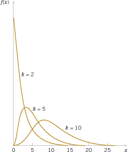
FIGURE 8-8 Probability density functions of several χ2 distributions.
The probability density function of a χ2 random variable is
![]()
where k is the number of degrees of freedom. The mean and variance of the χ2 distribution are k and 2k, respectively. Several chi-square distributions are shown in Fig. 8-8. Note that the chi-square random variable is non-negative and that the probability distribution is skewed to the right. However, as k increases, the distribution becomes more symmetric. As k → ∞, the limiting form of the chi-square distribution is the normal distribution.
The percentage points of the χ2 distribution are given in Table IV of the Appendix. Define ![]() as the percentage point or value of the chi-square random variable with k degrees of freedom such that the probability that X2 exceeds this value is α. That is,
as the percentage point or value of the chi-square random variable with k degrees of freedom such that the probability that X2 exceeds this value is α. That is,
![]()
This probability is shown as the shaded area in Fig. 8-9(a). To illustrate the use of Table IV, note that the areas α are the column headings and the degrees of freedom k are given in the left column. Therefore, the value with 10 degrees of freedom having an area (probability) of 0.05 to the right is ![]() = 18.31. This value is often called an upper 5% point of chi-square with 10 degrees of freedom. We may write this as a probability statement as follows:
= 18.31. This value is often called an upper 5% point of chi-square with 10 degrees of freedom. We may write this as a probability statement as follows:
![]()
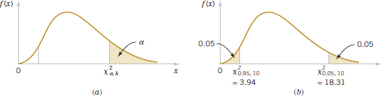
FIGURE 8-9 Percentage point of the χ2 distribution. (a) The percentage point ![]() . (b) The upper percentage point
. (b) The upper percentage point ![]() and the lower percentage point
and the lower percentage point ![]() .
.
Conversely, a lower 5% point of chi-square with 10 degrees of freedom would be ![]() = 3.94 (from Appendix A). Both of these percentage points are shown in Figure 8-9(b).
= 3.94 (from Appendix A). Both of these percentage points are shown in Figure 8-9(b).
The construction of the 100(1 − α)% CI for σ2 is straightforward. Because
![]()
is chi-square with n − 1 degrees of freedom, we may write
![]()
so that
![]()
This last equation can be rearranged as
![]()
This leads to the following definition of the confidence interval for σ2.
Confidence Interval on the Variance
If s2 is the sample variance from a random sample of n observations from a normal distribution with unknown variance σ2, then a 100(1 − α)% confidence interval on σ2 is
![]()
where ![]() and
and ![]() are the upper and lower 100α/2 percentage points of the chi-square distribution with n − 1 degrees of freedom, respectively. A confidence interval for σ has lower and upper limits that are the square roots of the corresponding limits in Equation 8-19.
are the upper and lower 100α/2 percentage points of the chi-square distribution with n − 1 degrees of freedom, respectively. A confidence interval for σ has lower and upper limits that are the square roots of the corresponding limits in Equation 8-19.
It is also possible to find a 100(1 − α)% lower confidence bound or upper confidence bound on σ2.
One-Sided Confidence Bounds on the Variance
The 100(1 − α)% lower and upper confidence bounds on σ2 are
![]()
respectively.
The CIs given in Equations 8-19 and 8-20 are less robust to the normality assumption. The distribution of (n − 1)S2/σ2 can be very different from the chi-square if the underlying population is not normal.
Example 8-7 Detergent Filling An automatic filling machine is used to fill bottles with liquid detergent. A random sample of 20 bottles results in a sample variance of fill volume of s2 = 0.01532 (fluid ounce). If the variance of fill volume is too large, an unacceptable proportion of bottles will be under- or overfilled. We will assume that the fill volume is approximately normally distributed. A 95% upper confidence bound is found from Equation 8-26 as follows:
![]()
![]()
This last expression may be converted into a confidence interval on the standard deviation σ by taking the square root of both sides, resulting in
![]()
Practical Interpretation: Therefore, at the 95% level of confidence, the data indicate that the process standard deviation could be as large as 0.17 fluid ounce. The process engineer or manager now needs to determine whether a standard deviation this large could lead to an operational problem with under- or over-filled bottles.
Exercises FOR SECTION 8-3
![]() Problem available in WileyPLUS at instructor's discretion.
Problem available in WileyPLUS at instructor's discretion.
![]() Go Tutorial Tutoring problem available in WileyPLUS at instructor's discretion
Go Tutorial Tutoring problem available in WileyPLUS at instructor's discretion
8-46. ![]() Determine the values of the following percentiles:
Determine the values of the following percentiles:
![]() .
.
8-47. Determine the χ2 percentile that is required to construct each of the following CIs:
(a) Confidence level = 95%, degrees of freedom = 24, one-sided (upper)
(b) Confidence level = 99%, degrees of freedom = 9, one-sided (lower)
(c) Confidence level = 90%, degrees of freedom = 19, two-sided.
8-48. ![]() A rivet is to be inserted into a hole. A random sample of n = 15 parts is selected, and the hole diameter is measured. The sample standard deviation of the hole diameter measurements is s = 0.008 millimeters. Construct a 99% lower confidence bound for σ2.
A rivet is to be inserted into a hole. A random sample of n = 15 parts is selected, and the hole diameter is measured. The sample standard deviation of the hole diameter measurements is s = 0.008 millimeters. Construct a 99% lower confidence bound for σ2.
8-49. Consider the situation in Exercise 8-48. Find a 99% lower confidence bound on the standard deviation.
8-50. ![]() The sugar content of the syrup in canned peaches is normally distributed. A random sample of n = 10 cans yields a sample standard deviation of s = 4.8 milligrams. Calculate a 95% two-sided confidence interval for σ.
The sugar content of the syrup in canned peaches is normally distributed. A random sample of n = 10 cans yields a sample standard deviation of s = 4.8 milligrams. Calculate a 95% two-sided confidence interval for σ.
8-51. ![]() The percentage of titanium in an alloy used in aerospace castings is measured in 51 randomly selected parts. The sample standard deviation is s = 0.37. Construct a 95% two-sided confidence interval for σ.
The percentage of titanium in an alloy used in aerospace castings is measured in 51 randomly selected parts. The sample standard deviation is s = 0.37. Construct a 95% two-sided confidence interval for σ.
8-52. ![]() An article in Medicine and Science in Sports and Exercise [“Electrostimulation Training Effects on the Physical Performance of Ice Hockey Players” (2005, Vol. 37, pp. 455–460)] considered the use of electromyostimulation (EMS) as a method to train healthy skeletal muscle. EMS sessions consisted of 30 contractions (4-second duration, 85 Hz) and were carried out three times per week for three weeks on 17 ice hockey players. The 10-meter skating performance test showed a standard deviation of 0.09 seconds. Construct a 95% confidence interval of the standard deviation of the skating performance test.
An article in Medicine and Science in Sports and Exercise [“Electrostimulation Training Effects on the Physical Performance of Ice Hockey Players” (2005, Vol. 37, pp. 455–460)] considered the use of electromyostimulation (EMS) as a method to train healthy skeletal muscle. EMS sessions consisted of 30 contractions (4-second duration, 85 Hz) and were carried out three times per week for three weeks on 17 ice hockey players. The 10-meter skating performance test showed a standard deviation of 0.09 seconds. Construct a 95% confidence interval of the standard deviation of the skating performance test.
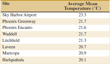
8-53. ![]() Go Tutorial An article in Urban Ecosystems, “Urbanization and Warming of Phoenix (Arizona, USA): Impacts, Feedbacks and Mitigation” (2002, Vol. 6, pp. 183–203), mentions that Phoenix is ideal to study the effects of an urban heat island because it has grown from a population of 300,000 to approximately 3 million over the last 50 years, which is a period with a continuous, detailed climate record. The 50-year averages of the mean annual temperatures at eight sites in Phoenix follow. Check the assumption of normality in the population with a probability plot. Construct a 95% confidence interval for the standard deviation over the sites of the mean annual temperatures.
Go Tutorial An article in Urban Ecosystems, “Urbanization and Warming of Phoenix (Arizona, USA): Impacts, Feedbacks and Mitigation” (2002, Vol. 6, pp. 183–203), mentions that Phoenix is ideal to study the effects of an urban heat island because it has grown from a population of 300,000 to approximately 3 million over the last 50 years, which is a period with a continuous, detailed climate record. The 50-year averages of the mean annual temperatures at eight sites in Phoenix follow. Check the assumption of normality in the population with a probability plot. Construct a 95% confidence interval for the standard deviation over the sites of the mean annual temperatures.
 .
.
8-54. ![]() An article in Cancer Research [“Analyses of Litter-Matched Time-to-Response Data, with Modifications for Recovery of Interlitter Information” (1977, Vol. 37, pp. 3863–3868)] tested the tumorigenesis of a drug. Rats were randomly selected from litters and given the drug. The times of tumor appearance were recorded as follows:
An article in Cancer Research [“Analyses of Litter-Matched Time-to-Response Data, with Modifications for Recovery of Interlitter Information” (1977, Vol. 37, pp. 3863–3868)] tested the tumorigenesis of a drug. Rats were randomly selected from litters and given the drug. The times of tumor appearance were recorded as follows:
![]()
Calculate a 95% confidence interval on the standard deviation of time until a tumor appearance. Check the assumption of normality of the population and comment on the assumptions for the confidence interval.
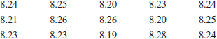
8-55. ![]() An article in Technometrics (1999, Vol. 41, pp. 202–211) studied the capability of a gauge by measuring the weight of paper. The data for repeated measurements of one sheet of paper are in the following table. Construct a 95% one-sided upper confidence interval for the standard deviation of these measurements. Check the assumption of normality of the data and comment on the assumptions for the confidence interval.
An article in Technometrics (1999, Vol. 41, pp. 202–211) studied the capability of a gauge by measuring the weight of paper. The data for repeated measurements of one sheet of paper are in the following table. Construct a 95% one-sided upper confidence interval for the standard deviation of these measurements. Check the assumption of normality of the data and comment on the assumptions for the confidence interval.

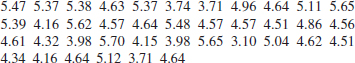
8-56. ![]() An article in the Australian Journal of Agricultural Research [“Non-Starch Polysaccharides and Broiler Performance on Diets Containing Soyabean Meal as the Sole Protein Concentrate” (1993, Vol. 44(8), pp. 1483–1499)] determined that the essential amino acid (Lysine) composition level of soybean meals is as shown here (g/kg):
An article in the Australian Journal of Agricultural Research [“Non-Starch Polysaccharides and Broiler Performance on Diets Containing Soyabean Meal as the Sole Protein Concentrate” (1993, Vol. 44(8), pp. 1483–1499)] determined that the essential amino acid (Lysine) composition level of soybean meals is as shown here (g/kg):
![]()
(a) Construct a 99% two-sided confidence interval for σ2.
(b) Calculate a 99% lower confidence bound for σ2.
(c) Calculate a 90% lower confidence bound for σ.
(d) Compare the intervals that you have computed.
8-57. From the data on the pH of rain in Ingham County, Michigan:
Find a two-sided 95% confidence interval for the standard deviation of pH.
8-58. From the data on CAT scans in Exercise 8-45
(a) Find a two-sided 95% confidence interval for the standard deviation.
(b) What should you do to address any reservations about the confidence interval you found in part (a)?
8-4 Large-Sample Confidence Interval for a Population Proportion
It is often necessary to construct confidence intervals on a population proportion. For example, suppose that a random sample of size n has been taken from a large (possibly infinite) population and that X(≤ n) observations in this sample belong to a class of interest. Then ![]() = X/n is a point estimator of the proportion of the population p that belongs to this class. Note that n and p are the parameters of a binomial distribution. Furthermore, from Chapter 4 we know that the sampling distribution of
= X/n is a point estimator of the proportion of the population p that belongs to this class. Note that n and p are the parameters of a binomial distribution. Furthermore, from Chapter 4 we know that the sampling distribution of ![]() is approximately normal with mean p and variance p(1 − p)/n, if p is not too close to either 0 or 1 and if n is relatively large. Typically, to apply this approximation we require that np and n(1 − p) be greater than or equal to 5. We will use the normal approximation in this section.
is approximately normal with mean p and variance p(1 − p)/n, if p is not too close to either 0 or 1 and if n is relatively large. Typically, to apply this approximation we require that np and n(1 − p) be greater than or equal to 5. We will use the normal approximation in this section.
Normal Approximation for a Binomial Proportion
If n is large, the distribution of
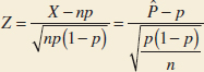
is approximately standard normal.
To construct the confidence interval on p, note that
![]()
so
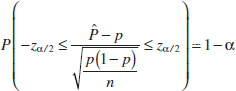
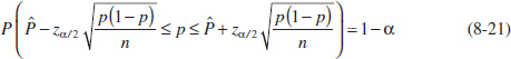
The quantity ![]() in Equation 8-21 is called the standard error of the point estimator
in Equation 8-21 is called the standard error of the point estimator ![]() . This was discussed in Chapter 7. Unfortunately, the upper and lower limits of the confidence interval obtained from Equation 8-21 contain the unknown parameter p. However, as suggested at the end of Section 8-1.5, a solution that is often satisfactory solution is to replace p by
. This was discussed in Chapter 7. Unfortunately, the upper and lower limits of the confidence interval obtained from Equation 8-21 contain the unknown parameter p. However, as suggested at the end of Section 8-1.5, a solution that is often satisfactory solution is to replace p by ![]() in the standard error, which results in
in the standard error, which results in
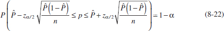
This leads to the approximate 100(1 − α)% confidence interval on p.
Approximate Confidence Interval on a Binomial Proportion
If ![]() is the proportion of observations in a random sample of size n that belongs to a class of interest, an approximate 100(1 − α)% confidence interval on the proportion p of the population that belongs to this class is
is the proportion of observations in a random sample of size n that belongs to a class of interest, an approximate 100(1 − α)% confidence interval on the proportion p of the population that belongs to this class is
![]()
where zα/2 is the upper α/2 percentage point of the standard normal distribution.
This procedure depends on the adequacy of the normal approximation to the binomial. To be reasonably conservative, this requires that np and n(1 − p) be greater than or equal to 5. In situations when this approximation is inappropriate, particularly in cases when n is small, other methods must be used. Tables of the binomial distribution could be used to obtain a confidence interval for p. However, we could also use numerical methods that are implemented on the binomial probability mass function in some computer program.
Example 8-8 Crankshaft Bearings In a random sample of 85 automobile engine crankshaft bearings, 10 have a surface finish that is rougher than the specifications allow. Therefore, a point estimate of the proportion of bearings in the population that exceeds the roughness specification is ![]() = x/n = 10/85 = 0.12. A 95% two-sided confidence interval for p is computed from Equation 8-23 as
= x/n = 10/85 = 0.12. A 95% two-sided confidence interval for p is computed from Equation 8-23 as
![]()
or
![]()
which simplifies to
![]()
Practical Interpretation: This is a wide CI. Although the sample size does not appear to be small (n = 85), the value of ![]() is fairly small, which leads to a large standard error for
is fairly small, which leads to a large standard error for ![]() contributing to the wide CI.
contributing to the wide CI.
Choice of Sample Size
Because ![]() is the point estimator of p, we can define the error in estimating p by
is the point estimator of p, we can define the error in estimating p by ![]() as E = |p −
as E = |p − ![]() |. Note that we are approximately 100(1 − α)% confident that this error is less than zα/2
|. Note that we are approximately 100(1 − α)% confident that this error is less than zα/2 ![]() . For instance, in Example 8-8, we are 95% confident that the sample proportion
. For instance, in Example 8-8, we are 95% confident that the sample proportion ![]() = 0.12 differs from the true proportion p by an amount not exceeding 0.07.
= 0.12 differs from the true proportion p by an amount not exceeding 0.07.
In situations when the sample size can be selected, we may choose n to be 100(1 − α)% confident that the error is less than some specified value E. If we set E = zα/2 ![]() and solve for n, the appropriate sample size is
and solve for n, the appropriate sample size is
Sample Size for a Specified Error on a Binomial Proportion
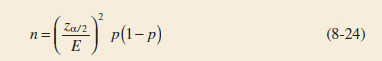
An estimate of p is required to use Equation 8-24. If an estimate ![]() from a previous sample is available, it can be substituted for p in Equation 8-24, or perhaps a subjective estimate can be made. If these alternatives are unsatisfactory, a preliminary sample can be taken,
from a previous sample is available, it can be substituted for p in Equation 8-24, or perhaps a subjective estimate can be made. If these alternatives are unsatisfactory, a preliminary sample can be taken, ![]() computed, and then Equation 8-24 used to determine how many additional observations are required to estimate p with the desired accuracy. Another approach to choosing n uses the fact that the sample size from Equation 8-24 will always be a maximum for p = 0.5 [that is, p(1 − p) ≤ 0.25 with equality for p = 0.5], and this can be used to obtain an upper bound on n. In other words, we are at least 100(1 − α)% confident that the error in estimating p by
computed, and then Equation 8-24 used to determine how many additional observations are required to estimate p with the desired accuracy. Another approach to choosing n uses the fact that the sample size from Equation 8-24 will always be a maximum for p = 0.5 [that is, p(1 − p) ≤ 0.25 with equality for p = 0.5], and this can be used to obtain an upper bound on n. In other words, we are at least 100(1 − α)% confident that the error in estimating p by ![]() is less than E if the sample size is
is less than E if the sample size is

Example 8-9 Crankshaft Bearings Consider the situation in Example 8-8. How large a sample is required if we want to be 95% confident that the error in using ![]() to estimate p is less than 0.05? Using
to estimate p is less than 0.05? Using ![]() = 0.12 as an initial estimate of p, we find from Equation 8-24 that the required sample size is
= 0.12 as an initial estimate of p, we find from Equation 8-24 that the required sample size is
![]()
If we wanted to be at least 95% confident that our estimate ![]() of the true proportion p was within 0.05 regardless of the value of p, we would use Equation 8-25 to find the sample size
of the true proportion p was within 0.05 regardless of the value of p, we would use Equation 8-25 to find the sample size
![]()
Practical Interpretation: Notice that if we have information concerning the value of p, either from a preliminary sample or from past experience, we could use a smaller sample while maintaining both the desired precision of estimation and the level of confidence.
One-Sided Confidence Bounds
We may find approximate one-sided confidence bounds on p by using a simple modification of Equation 8-23.
The approximate 100(1 − α)% lower and upper confidence bounds are
![]()
respectively.
A Different Cofidence interval on the Binomial Proportion
There is a different way to construct a CI on a binomial proportion than the traditional approach in Equation 8-23. Starting with Equation 8-22 and replacing the inequalities with an equality and solving the resulting quadratic equation for p results in
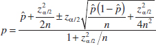
This implies that a two-sided CI on a proportion p is as follows:
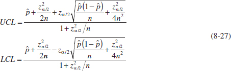
The article by Agresti and Coull in The American Statistician (“Approximate Better Than ‘Exact’ for Interval Estimation of a Binomial Proportion,” 1998, pp. 119–126) reports that the actual confidence level for the CI in Equation 8-27 is closer to the “advertised” or nominal level for almost all values of α and p than for the traditional CI in Equation 8-23. The authors also report that this new interval can be used with nearly all sample sizes. So the requirements that n![]() ≥ 5 or 10 or n(1 −
≥ 5 or 10 or n(1 − ![]() ) ≥ 5 or 10 are not too important. If the sample size is large, the quantity
) ≥ 5 or 10 are not too important. If the sample size is large, the quantity ![]() /(2n) will be small relative to
/(2n) will be small relative to ![]() ,
, ![]() /(4a2) will be small relative to
/(4a2) will be small relative to ![]() (1 −
(1 − ![]() )/n, and
)/n, and ![]() /n will be small, so as a result the Agresti-Coull CI in Equation 8-27 will reduce to the traditional CI given in Equation 8-23.
/n will be small, so as a result the Agresti-Coull CI in Equation 8-27 will reduce to the traditional CI given in Equation 8-23.
Example 8-10 The Agresti-Coull CI on a Proportion Reconsider the crankshaft bearing data introduced in Example 8-8. In that example we reported that ![]() = 0.12 and n = 85. The traditional 95% CI was
= 0.12 and n = 85. The traditional 95% CI was
![]()
To construct the new Agresti-Coull CI, we use Equation 8-27:
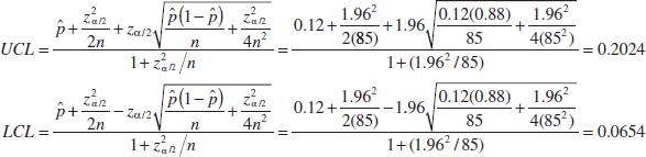
The two CIs would agree more closely if the sample size were larger.
![]() Problem available in WileyPLUS at instructor's discretion.
Problem available in WileyPLUS at instructor's discretion.
![]() Go Tutorial Tutoring problem available in WileyPLUS at instructor's discretion.
Go Tutorial Tutoring problem available in WileyPLUS at instructor's discretion.
8-59. ![]() The fraction of defective integrated circuits produced in a photolithography process is being studied. A random sample of 300 circuits is tested, revealing 13 defectives.
The fraction of defective integrated circuits produced in a photolithography process is being studied. A random sample of 300 circuits is tested, revealing 13 defectives.
(a) Calculate a 95% two-sided CI on the fraction of defective circuits produced by this particular tool.
(b) Calculate a 95% upper confidence bound on the fraction of defective circuits.
8-60. ![]() An article in Knee Surgery, Sports Traumatology, Arthroscopy [“Arthroscopic Meniscal Repair with an Absorbable Screw: Results and Surgical Technique” (2005, Vol. 13, pp. 273–279)] showed that only 25 out of 37 tears (67.6%) located between 3 and 6 mm from the meniscus rim were healed.
An article in Knee Surgery, Sports Traumatology, Arthroscopy [“Arthroscopic Meniscal Repair with an Absorbable Screw: Results and Surgical Technique” (2005, Vol. 13, pp. 273–279)] showed that only 25 out of 37 tears (67.6%) located between 3 and 6 mm from the meniscus rim were healed.
(a) Calculate a two-sided 95% confidence interval on the proportion of such tears that will heal.
(b) Calculate a 95% lower confidence bound on the proportion of such tears that will heal.
8-61. ![]() The 2004 presidential election exit polls from the critical state of Ohio provided the following results. The exit polls had 2020 respondents, 768 of whom were college graduates. Of the college graduates, 412 voted for George Bush.
The 2004 presidential election exit polls from the critical state of Ohio provided the following results. The exit polls had 2020 respondents, 768 of whom were college graduates. Of the college graduates, 412 voted for George Bush.
(a) Calculate a 95% confidence interval for the proportion of college graduates in Ohio who voted for George Bush.
(b) Calculate a 95% lower confidence bound for the proportion of college graduates in Ohio who voted for George Bush.
8-62. ![]() Of 1000 randomly selected cases of lung cancer, 823 resulted in death within 10 years.
Of 1000 randomly selected cases of lung cancer, 823 resulted in death within 10 years.
(a) Calculate a 95% two-sided confidence interval on the death rate from lung cancer.
(b) Using the point estimate of p obtained from the preliminary sample, what sample size is needed to be 95% confident that the error in estimating the true value of p is less than 0.03?
(c) How large must the sample be if you wish to be at least 95% confident that the error in estimating p is less than 0.03, regardless of the true value of p?
8-63. ![]() An article in the Journal of the American Statistical Association (1990, Vol. 85, pp. 972–985) measured the weight of 30 rats under experiment controls. Suppose that 12 were underweight rats.
An article in the Journal of the American Statistical Association (1990, Vol. 85, pp. 972–985) measured the weight of 30 rats under experiment controls. Suppose that 12 were underweight rats.
(a) Calculate a 95% two-sided confidence interval on the true proportion of rats that would show underweight from the experiment.
(b) Using the point estimate of p obtained from the preliminary sample, what sample size is needed to be 95% confident that the error in estimating the true value of p is less than 0.02?
(c) How large must the sample be if you wish to be at least 95% confident that the error in estimating p is less than 0.02, regardless of the true value of p?
8-64. ![]() A random sample of 50 suspension helmets used by motorcycle riders and automobile race-car drivers was subjected to an impact test, and some damage was observed on 18 of these helmets.
A random sample of 50 suspension helmets used by motorcycle riders and automobile race-car drivers was subjected to an impact test, and some damage was observed on 18 of these helmets.
(a) Find a 95% two-sided confidence interval on the true proportion of helmets that would show damage from this test.
(b) Using the point estimate of p from the 50 helmets, how many helmets must be tested to be 95% confident that the error in estimating p is less than 0.02?
(c) How large must the sample be if we wish to be at least 95% confident that the error in estimating p is less than 0.02 regardless of the true value of p?
8-65. ![]() The Arizona Department of Transportation wishes to survey state residents to determine what proportion of the population would like to increase statewide highway speed limits from 65 mph to 75 mph. How many residents does the department need to survey if it wants to be at least 99% confident that the sample proportion is within 0.05 of the true proportion?
The Arizona Department of Transportation wishes to survey state residents to determine what proportion of the population would like to increase statewide highway speed limits from 65 mph to 75 mph. How many residents does the department need to survey if it wants to be at least 99% confident that the sample proportion is within 0.05 of the true proportion?
8-66. ![]() A study is to be conducted of the percentage of homeowners who own at least two television sets. How large a sample is required if we wish to be 99% confident that the error in estimating this quantity is less than 0.017?
A study is to be conducted of the percentage of homeowners who own at least two television sets. How large a sample is required if we wish to be 99% confident that the error in estimating this quantity is less than 0.017?
8-67. The U.S. Postal Service (USPS) has used optical character recognition (OCR) since the mid-1960s. In 1983, USPS began deploying the technology to major post offices throughout the country (www.britannica.com). Suppose that in a random sample of 500 handwritten zip code digits, 466 were read correctly.
(a) Construct a 95% confidence interval for the true proportion of correct digits that can be automatically read.
(b) What sample size is needed to reduce the margin of error to 1%?
(c) How would the answer to part (b) change if you had to assume that the machine read only one-half of the digits correctly?
8-68. Information on a packet of seeds claims that 93% of them will germinate. Of the 200 seeds that I planted, only 180 germinated.
(a) Find a 95% confidence interval for the true proportion of seeds that germinate based on this sample.
(b) Does this seem to provide evidence that the claim is wrong?
8-69. Use the data from Exercise 8-59 to compute a two-sided Agresti-Coull CI on the proportion of defective circuits. Compare and discuss the CI to the one computed in Exercise 8-59.
8-70. Use the data from Exercise 8-60 to compute a two-sided Agresti-Coull CI on the proportion of tears that will heal. Compare and discuss the CI to the one computed in Exercise 8-60.
8-71. Use the data from Exercise 8-66 to compute a two-sided Agresti-Coull CI on the proportion of correct digits that can be automatically read. Compare and discuss the CI to the one computed in Exercise 8-66.
8-72. Use the data from Exercise 8-68 to compute a two-sided Agresti-Coull CI on the proportion of seeds that germinate. Compare and discuss the CI to the one computed in Exercise 8-68.
8-5 Guidelines for Constructing Confidence Intervals
The most difficult step in constructing a confidence interval is often the match of the appropriate calculation to the objective of the study. Common cases are listed in Table 8-1 along with the reference to the section that covers the appropriate calculation for a confidence interval test. Table 8-1 provides a simple road map to help select the appropriate analysis. Two primary comments can help identify the analysis:
- Determine the parameter (and the distribution of the data) that will be bounded by the confidence interval or tested by the hypothesis.
- Check if other parameters are known or need to be estimated.
![]() TABLE • 8-1 The Roadmap for Constructing Confidence Intervals and Performing Hypothesis Tests, One-Sample Case
TABLE • 8-1 The Roadmap for Constructing Confidence Intervals and Performing Hypothesis Tests, One-Sample Case
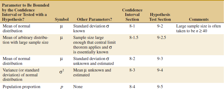
In Chapter 9, we will study a procedure closely related to confidence intervals called hypothesis testing. Table 8-1 can be used for those procedures also. This road map will be extended to more cases in Chapter 10.
8.6 Bootstrap Confidence Interval
In Section 7-3.4, we saw how a computer-intensive technique called the bootstrap could be used to find the estimated standard error of a statistic, say ![]() . The bootstrap technique can also be used to find confidence intervals. These bootstrap can be useful in situations in which a “standard” CI is not readily available. To illustrate the general approach, let's consider a case for which there is a standard CI, the 100(1 − α)% CI on the mean of a normal distribution with known variance. Here the parameter of interest is the population mean μ, and the statistic that estimates μ is the sample average
. The bootstrap technique can also be used to find confidence intervals. These bootstrap can be useful in situations in which a “standard” CI is not readily available. To illustrate the general approach, let's consider a case for which there is a standard CI, the 100(1 − α)% CI on the mean of a normal distribution with known variance. Here the parameter of interest is the population mean μ, and the statistic that estimates μ is the sample average ![]() . The quantity zα/2σ/
. The quantity zα/2σ/![]() is the 100(1 − α / 2) percentile of the distribution of
is the 100(1 − α / 2) percentile of the distribution of ![]() , i = 1, 2,..., nB and by the same logic, the quantity − zα/2σ/
, i = 1, 2,..., nB and by the same logic, the quantity − zα/2σ/![]() is the 100(α/2) percentile of the distribution of
is the 100(α/2) percentile of the distribution of ![]() − μ. Therefore, the 100(1 − α/2)% CI can be written as:
− μ. Therefore, the 100(1 − α/2)% CI can be written as:
![]()
This can be rearranged as
![]()
So the lower confidence bound is ![]() − (1 − α/2)th percentile of the distribution of
− (1 − α/2)th percentile of the distribution of ![]() − μ and the upper confidence bound is
− μ and the upper confidence bound is ![]() + α/2th percentile of the distribution of
+ α/2th percentile of the distribution of ![]() − μ. When these percentiles cannot be easily determined for some arbitrary parameter θ, they can often be estimated by using bootstrap samples. The procedure would consist of taking nB bootstrap samples, calculating the bootstrap estimates
− μ. When these percentiles cannot be easily determined for some arbitrary parameter θ, they can often be estimated by using bootstrap samples. The procedure would consist of taking nB bootstrap samples, calculating the bootstrap estimates ![]() and
and ![]() , and then computing the differences
, and then computing the differences ![]() , i = 1,2,...,nB. The α/2 smallest and largest of these differences are the estimates of the percentiles required to construct the bootstrap CI.
, i = 1,2,...,nB. The α/2 smallest and largest of these differences are the estimates of the percentiles required to construct the bootstrap CI.
8-7 Tolerance and Prediction Intervals
8-7.1 PREDICTION INTERVAL FOR A FUTURE OBSERVATION
In some problem situations, we may be interested in predicting a future observation of a variable. This is a different problem than estimating the mean of that variable, so a confidence interval is not appropriate. In this section, we show how to obtain a 100(1 − α)% prediction interval on a future value of a normal random variable.
Suppose that X1, X2,..., Xn is a random sample from a normal population. We wish to predict the value Xn+1, a single future observation. A point prediction of Xn+1 is ![]() , the sample mean. The prediction error is Xn+1 −
, the sample mean. The prediction error is Xn+1 − ![]() . The expected value of the prediction error is
. The expected value of the prediction error is
![]()
and the variance of the prediction error is
![]()
because the future observation Xn+1 is independent of the mean of the current sample ![]() . The prediction error Xn+1 −
. The prediction error Xn+1 − ![]() is normally distributed. Therefore,
is normally distributed. Therefore,

has a standard normal distribution. Replacing σ with S results in

which has a t distribution with n − 1 degrees of freedom. Manipulating T as we have done previously in the development of a CI leads to a prediction interval on the future observation Xn+1.
Prediction Interval
A 100(1 − α)% prediction interval (PI) on a single future observation from a normal distribution is given by
![]()
The prediction interval for Xn+1 will always be longer than the confidence interval for μ because more variability is associated with the prediction error than with the error of estimation. This is easy to see because the prediction error is the difference between two random variables (Xn+1 − ![]() ), and the estimation error in the CI is the difference between one random variable and a constant (
), and the estimation error in the CI is the difference between one random variable and a constant (![]() − μ). As n gets larger (n → ∞), the length of the CI decreases to zero, essentially becoming the single value μ, but the length of the PI approaches 2zα/2σ. So as n increases, the uncertainty in estimating μ goes to zero, although there will always be uncertainty about the future value Xn+1, even when estimating any of the distribution parameters is not necessary.
− μ). As n gets larger (n → ∞), the length of the CI decreases to zero, essentially becoming the single value μ, but the length of the PI approaches 2zα/2σ. So as n increases, the uncertainty in estimating μ goes to zero, although there will always be uncertainty about the future value Xn+1, even when estimating any of the distribution parameters is not necessary.
We noted in Section 8-2 that the t distribution based CI for μ was robust to the normality assumption when n is small. The practical implication of this is that although we have computed a 95% CI, the actual confidence level will not be exactly 95%, but it will be very close—maybe 93% or 94%. Prediction intervals, on the other hand, are very sensitive to the normality assumption, and Equaion 8-28 should not be used unless we are very comfortable with the normality assumption.
Example 8-11 Alloy Adhesion Reconsider the tensile adhesion tests on specimens of U-700 alloy described in Example 8-6. The load at failure for n = 22 specimens was observed, and we found that ![]() = 13.71 and s = 3.55. The 95% confidence interval on μ was 12.14 ≤ μ ≤ 15.28. We plan to test a 23rd specimen. A 95% prediction interval on the load at failure for this specimen is
= 13.71 and s = 3.55. The 95% confidence interval on μ was 12.14 ≤ μ ≤ 15.28. We plan to test a 23rd specimen. A 95% prediction interval on the load at failure for this specimen is
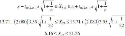
Practical Interpretation: Notice that the prediction interval is considerably longer than the CI. This is because the CI is an estimate of a parameter, but the PI is an interval estimate of a single future observation.
8-7.2 TOLERANCE INTERVAL FOR A NORMAL DISTRIBUTION
Consider a population of semiconductor processors. Suppose that the speed of these processors has a normal distribution with mean μ = 600 megahertz and standard deviation σ = 30 megahertz. Then the interval from 600 − 1.96(30) = 541.2 to 600 + 1.96(30) = 658.8 megahertz captures the speed of 95% of the processors in this population because the interval from −1.96 to 1.96 captures 95% of the area under the standard normal curve. The interval from μ − zα/2σ to μ + zα/2σ is called a tolerance interval.
If μ and σ are unknown, we can use the data from a random sample of size n to compute ![]() and s and then form the interval (
and s and then form the interval (![]() − 1.96 s,
− 1.96 s, ![]() + 1.96 s). However, because of sampling variability in
+ 1.96 s). However, because of sampling variability in ![]() and s, it is likely that this interval will contain less than 95% of the values in the population. The solution to this problem is to replace 1.96 with some value that will make the proportion of the distribution contained in the interval 95% with some level of confidence. Fortunately, it is easy to do this.
and s, it is likely that this interval will contain less than 95% of the values in the population. The solution to this problem is to replace 1.96 with some value that will make the proportion of the distribution contained in the interval 95% with some level of confidence. Fortunately, it is easy to do this.
Tolerance Interval
A tolerance interval for capturing at least γ% of the values in a normal distribution with confidence level 100(1 − α)% is
![]()
where k is a tolerance interval factor found in Appendix Table XII. Values are given for γ = 90%, 95%, and 99%, and for 90%, 95%, and 99% confidence.
This interval is very sensitive to the normality assumption. One-sided tolerance bounds can also be computed. The tolerance factors for these bounds are also given in Appendix Table XII.
Example 8-12 Alloy Adhesion Let's reconsider the tensile adhesion tests originally described in Example 8-6. The load at failure for n = 22 specimens was observed, and we found that ![]() = 13.71 and s = 3.55. We want to find a tolerance interval for the load at failure that includes 90% of the values in the population with 95% confidence. From Appendix Table XII, the tolerance factor k for n = 22, γ = 0.90, and 95% confidence is k = 2.264. The desired tolerance interval is
= 13.71 and s = 3.55. We want to find a tolerance interval for the load at failure that includes 90% of the values in the population with 95% confidence. From Appendix Table XII, the tolerance factor k for n = 22, γ = 0.90, and 95% confidence is k = 2.264. The desired tolerance interval is
![]()
or
![]()
which reduces to (5.67, 21.74).
Practical Interpretation: We can be 95% confident that at least 90% of the values of load at failure for this particular alloy lie between 5.67 and 21.74 megapascals.
From Appendix Table XII, we note that as n → ∞, the value of k goes to the z-value associated with the desired level of containment for the normal distribution. For example, if we want 90% of the population to fall in the two-sided tolerance interval, k approaches z0.05 = 1.645 as n → ∞. Note that as n → ∞, a 100(1 − α)% prediction interval on a future value approaches a tolerance interval that contains 100(1 − α)% of the distribution.
Exercises FOR SECTION 8-6
![]() Problem available in WileyPLUS at instructor's discretion.
Problem available in WileyPLUS at instructor's discretion.
![]() Go Tutorial Tutoring problem available in WileyPLUS at instructor's discretion.
Go Tutorial Tutoring problem available in WileyPLUS at instructor's discretion.
8-73. ![]() Go Tutorial Consider the tire-testing data described in Exercise 8-29. Compute a 95% prediction interval on the life of the next tire of this type tested under conditions that are similar to those employed in the original test. Compare the length of the prediction interval with the length of the 95% CI on the population mean.
Go Tutorial Consider the tire-testing data described in Exercise 8-29. Compute a 95% prediction interval on the life of the next tire of this type tested under conditions that are similar to those employed in the original test. Compare the length of the prediction interval with the length of the 95% CI on the population mean.
8-74. Consider the Izod impact test described in Exercise 8-30. Compute a 99% prediction interval on the impact strength of the next specimen of PVC pipe tested. Compare the length of the prediction interval with the length of the 99% CI on the population mean.
8-75. ![]() Consider the syrup-dispensing measurements described in Exercise 8-31. Compute a 95% prediction interval on the syrup volume in the next beverage dispensed. Compare the length of the prediction interval with the length of the 95% CI on the population mean.
Consider the syrup-dispensing measurements described in Exercise 8-31. Compute a 95% prediction interval on the syrup volume in the next beverage dispensed. Compare the length of the prediction interval with the length of the 95% CI on the population mean.
8-76. Consider the natural frequency of beams described in Exercise 8-34. Compute a 90% prediction interval on the diameter of the natural frequency of the next beam of this type that will be tested. Compare the length of the prediction interval with the length of the 90% CI on the population mean.
8-77. ![]() Consider the rainfall in Exercise 8-35. Compute a 95% prediction interval on the rainfall for the next year. Compare the length of the prediction interval with the length of the 95% CI on the population mean.
Consider the rainfall in Exercise 8-35. Compute a 95% prediction interval on the rainfall for the next year. Compare the length of the prediction interval with the length of the 95% CI on the population mean.
8-78. Consider the margarine test described in Exercise 8-38. Compute a 99% prediction interval on the polyunsaturated fatty acid in the next package of margarine that is tested. Compare the length of the prediction interval with the length of the 99% CI on the population mean.
8-79. ![]() Consider the television tube brightness test described in Exercise 8-37. Compute a 99% prediction interval on the brightness of the next tube tested. Compare the length of the prediction interval with the length of the 99% CI on the population mean.
Consider the television tube brightness test described in Exercise 8-37. Compute a 99% prediction interval on the brightness of the next tube tested. Compare the length of the prediction interval with the length of the 99% CI on the population mean.
8-80. ![]() Consider the suspension rod diameter measurements described in Exercise 8-40. Compute a 95% prediction interval on the diameter of the next rod tested. Compare the length of the prediction interval with the length of the 95% CI on the population mean.
Consider the suspension rod diameter measurements described in Exercise 8-40. Compute a 95% prediction interval on the diameter of the next rod tested. Compare the length of the prediction interval with the length of the 95% CI on the population mean.
8-81. ![]() Consider the test on the compressive strength of concrete described in Exercise 8-39. Compute a 90% prediction interval on the next specimen of concrete tested.
Consider the test on the compressive strength of concrete described in Exercise 8-39. Compute a 90% prediction interval on the next specimen of concrete tested.
8-82. ![]() Go Tutorial Consider the bottle-wall thickness measurements described in Exercise 8-42. Compute a 90% prediction interval on the wall thickness of the next bottle tested.
Go Tutorial Consider the bottle-wall thickness measurements described in Exercise 8-42. Compute a 90% prediction interval on the wall thickness of the next bottle tested.
8-83. ![]() Consider the fuel rod enrichment data described in Exercise 8-43. Compute a 90% prediction interval on the enrichment of the next rod tested. Compare the length of the prediction interval with the length of the 99% CI on the population mean.
Consider the fuel rod enrichment data described in Exercise 8-43. Compute a 90% prediction interval on the enrichment of the next rod tested. Compare the length of the prediction interval with the length of the 99% CI on the population mean.
8-84. How would you obtain a one-sided prediction bound on a future observation? Apply this procedure to obtain a 95% one-sided prediction bound on the wall thickness of the next bottle for the situation described in Exercise 8-42.
8-85. Consider the tire-testing data in Exercise 8-29. Compute a 95% tolerance interval on the life of the tires that has confidence level 95%. Compare the length of the tolerance interval with the length of the 95% CI on the population mean. Which interval is shorter? Discuss the difference in interpretation of these two intervals.
8-86. ![]() Consider the Izod impact test described in Exercise 8-30. Compute a 99% tolerance interval on the impact strength of PVC pipe that has confidence level 90%. Compare the length of the tolerance interval with the length of the 99% CI on the population mean. Which interval is shorter? Discuss the difference in interpretation of these two intervals.
Consider the Izod impact test described in Exercise 8-30. Compute a 99% tolerance interval on the impact strength of PVC pipe that has confidence level 90%. Compare the length of the tolerance interval with the length of the 99% CI on the population mean. Which interval is shorter? Discuss the difference in interpretation of these two intervals.
8-87. ![]() Consider the syrup-volume data in Exercise 8-31. Compute a 95% tolerance interval on the syrup volume that has confidence level 90%. Compare the length of the tolerance interval with the length of the 95% CI on the population mean.
Consider the syrup-volume data in Exercise 8-31. Compute a 95% tolerance interval on the syrup volume that has confidence level 90%. Compare the length of the tolerance interval with the length of the 95% CI on the population mean.
8-88. ![]() Consider the margarine test described in Exercise 8-38. Compute a 99% tolerance interval on the polyunsaturated fatty acid in this particular type of margarine that has confidence level 95%. Compare the length of the tolerance interval with the length of the 99% CI on the population mean. Which interval is shorter? Discuss the difference in interpretation of these two intervals.
Consider the margarine test described in Exercise 8-38. Compute a 99% tolerance interval on the polyunsaturated fatty acid in this particular type of margarine that has confidence level 95%. Compare the length of the tolerance interval with the length of the 99% CI on the population mean. Which interval is shorter? Discuss the difference in interpretation of these two intervals.
8-89. Consider the rainfall data in Exercise 8-35. Compute a 95% tolerance interval that has confidence level 95%. Compare the length of the tolerance interval with the length of the 95% CI on the population mean. Discuss the difference in interpretation of these two intervals.
8-90. ![]() Consider the suspension rod diameter data in Exercise 8-40. Compute a 95% tolerance interval on the diameter of the rods described that has 90% confidence. Compare the length of the tolerance interval with the length of the 95% CI on the population mean. Which interval is shorter? Discuss the difference in interpretation of these two intervals.
Consider the suspension rod diameter data in Exercise 8-40. Compute a 95% tolerance interval on the diameter of the rods described that has 90% confidence. Compare the length of the tolerance interval with the length of the 95% CI on the population mean. Which interval is shorter? Discuss the difference in interpretation of these two intervals.
8-91. Consider the television tube brightness data in Exercise 8-37. Compute a 99% tolerance interval on the brightness of the television tubes that has confidence level 95%. Compare the length of the tolerance interval with the length of the 99% CI on the population mean. Which interval is shorter? Discuss the difference in interpretation of these two intervals.
8-92. Consider the strength-of-concrete data in Exercise 8-39. Compute a 90% tolerance interval on the compressive strength of the concrete that has 90% confidence.
8-93. Consider the fuel rod enrichment data described in Exercise 8-43. Compute a 99% tolerance interval on rod enrichment that has confidence level 95%. Compare the length of the tolerance interval with the length of the 95% CI on the population mean.
8-94. ![]() Consider the bottle-wall thickness measurements described in Exercise 8-42.
Consider the bottle-wall thickness measurements described in Exercise 8-42.
(a) Compute a 90% tolerance interval on bottle-wall thickness that has confidence level 90%.
(b) Compute a 90% lower tolerance bound on bottle-wall thickness that has confidence level 90%. Why would a lower tolerance bound likely be of interest here?
Supplemental Exercises
![]() Problem available in WileyPLUS at instructor's discretion.
Problem available in WileyPLUS at instructor's discretion.
![]() Go Tutorial Tutoring problem available in WileyPLUS at instructor's discretion.
Go Tutorial Tutoring problem available in WileyPLUS at instructor's discretion.
8-95. Consider the confidence interval for μ with known standard deviation σ:
![]()
where α1 + α2 = α. Let α = 0.05 and find the interval for α1 = α2 = α/2 = 0.025. Now find the interval for the case α1 = 0.01 and α2 = 0.04. Which interval is shorter? Is there any advantage to a “symmetric” confidence interval?
8-96. A normal population has a known mean of 50 and unknown variance.
(a) A random sample of n = 16 is selected from this population, and the sample results are ![]() = 52 and s = 8. How unusual are these results? That is, what is the probability of observing a sample average as large as 52 (or larger) if the known, underlying mean is actually 50?
= 52 and s = 8. How unusual are these results? That is, what is the probability of observing a sample average as large as 52 (or larger) if the known, underlying mean is actually 50?
(b) A random sample of n = 30 is selected from this population, and the sample results are ![]() = 52 and s = 8. How unusual are these results?
= 52 and s = 8. How unusual are these results?
(c) A random sample of n = 100 is selected from this population, and the sample results are ![]() = 52 and s = 8. How unusual are these results?
= 52 and s = 8. How unusual are these results?
(d) Compare your answers to parts (a)–(c) and explain why they are the same or different.
8-97. A normal population has known mean μ = 50 and variance σ2 = 5. What is the approximate probability that the sample variance is greater than or equal to 7.44? less than or equal to 2.56? For a random sample of size
(a) n = 16
(b) n = 30
(c) n = 71
(d) Compare your answers to parts (a)–(c) for the approximate probability that the sample variance is greater than or equal to 7.44. Explain why this tail probability is increasing or decreasing with increased sample size.
(e) Compare your answers to parts (a)–(c) for the approximate probability that the sample variance is less than or equal to 2.56. Explain why this tail probability is increasing or decreasing with increased sample size.
8-98. ![]() An article in the Journal of Sports Science (1987, Vol. 5, pp. 261–271) presents the results of an investigation of the hemoglobin level of Canadian Olympic ice hockey players. The data reported are as follows (in g/dl):
An article in the Journal of Sports Science (1987, Vol. 5, pp. 261–271) presents the results of an investigation of the hemoglobin level of Canadian Olympic ice hockey players. The data reported are as follows (in g/dl):
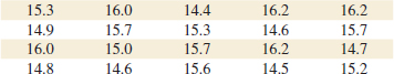
(a) Given the following probability plot of the data, what is a logical assumption about the underlying distribution of the data?
(b) Explain why this check of the distribution underlying the sample data is important if you want to construct a confidence interval on the mean.
(c) Based on this sample data, a 95% confidence interval for the mean is (15.04, 15.62). Is it reasonable to infer that the true mean could be 14.5? Explain your answer.
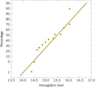
(d) Explain why this check of the distribution underlying the sample data is important if we want to construct a confidence interval on the variance.
(e) Based on these sample data, a 95% confidence interval for the variance is (0.22, 0.82). Is it reasonable to infer that the true variance could be 0.35? Explain your answer.
(f) Is it reasonable to use these confidence intervals to draw an inference about the mean and variance of hemoglobin levels
(i) of Canadian doctors? Explain your answer.
(ii) of Canadian children ages 6–12? Explain your answer.
8-99. The article “Mix Design for Optimal Strength Development of Fly Ash Concrete” (Cement and Concrete Research, 1989, Vol. 19(4), pp. 634–640) investigates the compressive strength of concrete when mixed with fly ash (a mixture of silica, alumina, iron, magnesium oxide, and other ingredients). The compressive strength for nine samples in dry conditions on the 28th day are as follows (in megapascals):
![]()
(a) Given the following probability plot of the data, what is a logical assumption about the underlying distribution of the data?
(b) Find a 99% lower one-sided confidence interval on mean compressive strength. Provide a practical interpretation of this interval.
(c) Find a 98% two-sided confidence interval on mean compressive strength. Provide a practical interpretation of this interval and explain why the lower end-point of the interval is or is not the same as in part (b).
(d) Find a 99% upper one-sided confidence interval on the variance of compressive strength. Provide a practical interpretation of this interval.
(e) Find a 98% two-sided confidence interval on the variance of compression strength. Provide a practical interpretation of this interval and explain why the upper end-point of the interval is or is not the same as in part (d).
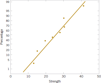
(f) Suppose that it was discovered that the largest observation 40.2 was misrecorded and should actually be 20.4. Now the sample mean ![]() = 23 and the sample variance s2 = 39.8. Use these new values and repeat parts (c) and (e). Compare the original computed intervals and the newly computed intervals with the corrected observation value. How does this mistake affect the values of the sample mean, sample variance, and the width of the two-sided confidence intervals?
= 23 and the sample variance s2 = 39.8. Use these new values and repeat parts (c) and (e). Compare the original computed intervals and the newly computed intervals with the corrected observation value. How does this mistake affect the values of the sample mean, sample variance, and the width of the two-sided confidence intervals?
(g) Suppose, instead, that it was discovered that the largest observation 40.2 is correct but that the observation 25.8 is incorrect and should actually be 24.8. Now the sample mean ![]() = 25 and the standard deviation s = 8.41. Use these new values and repeat parts (c) and (e). Compare the original computed intervals and the newly computed intervals with the corrected observation value. How does this mistake affect the values of the sample mean, the sample variance, and the width of the two-sided confidence intervals?
= 25 and the standard deviation s = 8.41. Use these new values and repeat parts (c) and (e). Compare the original computed intervals and the newly computed intervals with the corrected observation value. How does this mistake affect the values of the sample mean, the sample variance, and the width of the two-sided confidence intervals?
(h) Use the results from parts (f) and (g) to explain the effect of mistakenly recorded values on sample estimates. Comment on the effect when the mistaken values are near the sample mean and when they are not.
8-100. ![]() An operating system for a personal computer has been studied extensively, and it is known that the standard deviation of the response time following a particular command is σ = 8 milliseconds. A new version of the operating system is installed, and you wish to estimate the mean response time for the new system to ensure that a 95% confidence interval for μ has a length of at most 5 milliseconds.
An operating system for a personal computer has been studied extensively, and it is known that the standard deviation of the response time following a particular command is σ = 8 milliseconds. A new version of the operating system is installed, and you wish to estimate the mean response time for the new system to ensure that a 95% confidence interval for μ has a length of at most 5 milliseconds.
(a) If you can assume that response time is normally distributed and that σ = 8 for the new system, what sample size would you recommend?
(b) Suppose that the vendor tells you that the standard deviation of the response time of the new system is smaller, say, σ = 6; give the sample size that you recommend and comment on the effect the smaller standard deviation has on this calculation.
8-101. ![]() Consider the hemoglobin data in Exercise 8-97. Find the following:
Consider the hemoglobin data in Exercise 8-97. Find the following:
(a) An interval that contains 95% of the hemoglobin values with 90% confidence.
(b) An interval that contains 99% of the hemoglobin values with 90% confidence.
8-102. ![]() Consider the compressive strength of concrete data from Exercise 8-99. Find a 95% prediction interval on the next sample that will be tested.
Consider the compressive strength of concrete data from Exercise 8-99. Find a 95% prediction interval on the next sample that will be tested.
8-103. The maker of a shampoo knows that customers like this product to have a lot of foam. Ten sample bottles of the product are selected at random and the foam heights observed are as follows (in millimeters): 210, 215, 194, 195, 211, 201, 198, 204, 208, and 196.
(a) Is there evidence to support the assumption that foam height is normally distributed?
(b) Find a 95% CI on the mean foam height.
(c) Find a 95% prediction interval on the next bottle of shampoo that will be tested.
(d) Find an interval that contains 95% of the shampoo foam heights with 99% confidence.
(e) Explain the difference in the intervals computed in parts (b), (c), and (d).
8-104. During the 1999 and 2000 baseball seasons, there was much speculation that the unusually large number of home runs hit was due at least in part to a livelier ball. One way to test the “liveliness” of a baseball is to launch the ball at a vertical surface with a known velocity VL and measure the ratio of the outgoing velocity VO of the ball to VL. The ratio R = VO/VL is called the coefficient of restitution. Following are measurements of the coefficient of restitution for 40 randomly selected baseballs. The balls were thrown from a pitching machine at an oak surface.
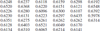
(a) Is there evidence to support the assumption that the coefficient of restitution is normally distributed?
(b) Find a 99% CI on the mean coefficient of restitution.
(c) Find a 99% prediction interval on the coefficient of restitution for the next baseball that will be tested.
(d) Find an interval that will contain 99% of the values of the coefficient of restitution with 95% confidence.
(e) Explain the difference in the three intervals computed in parts (b), (c), and (d).
8-105. ![]() Consider the baseball coefficient of restitution data in Exercise 8-104. Suppose that any baseball that has a coefficient of restitution that exceeds 0.635 is considered too lively. Based on the available data, what proportion of the baseballs in the sampled population are too lively? Find a 95% lower confidence bound on this proportion.
Consider the baseball coefficient of restitution data in Exercise 8-104. Suppose that any baseball that has a coefficient of restitution that exceeds 0.635 is considered too lively. Based on the available data, what proportion of the baseballs in the sampled population are too lively? Find a 95% lower confidence bound on this proportion.
8-106. ![]() An article in the ASCE Journal of Energy Engineering [“Overview of Reservoir Release Improvements at 20 TVA Dams” (Vol. 125, April 1999, pp. 1–17)] presents data on dissolved oxygen concentrations in streams below 20 dams in the Tennessee Valley Authority system. The observations are (in milligrams per liter): 5.0, 3.4, 3.9, 1.3, 0.2, 0.9, 2.7, 3.7, 3.8, 4.1, 1.0, 1.0, 0.8, 0.4, 3.8, 4.5, 5.3, 6.1, 6.9, and 6.5.
An article in the ASCE Journal of Energy Engineering [“Overview of Reservoir Release Improvements at 20 TVA Dams” (Vol. 125, April 1999, pp. 1–17)] presents data on dissolved oxygen concentrations in streams below 20 dams in the Tennessee Valley Authority system. The observations are (in milligrams per liter): 5.0, 3.4, 3.9, 1.3, 0.2, 0.9, 2.7, 3.7, 3.8, 4.1, 1.0, 1.0, 0.8, 0.4, 3.8, 4.5, 5.3, 6.1, 6.9, and 6.5.
(a) Is there evidence to support the assumption that the dissolved oxygen concentration is normally distributed?
(b) Find a 95% CI on the mean dissolved oxygen concentration.
(c) Find a 95% prediction interval on the dissolved oxygen concentration for the next stream in the system that will be tested.
(d) Find an interval that will contain 95% of the values of the dissolved oxygen concentration with 99% confidence.
(e) Explain the difference in the three intervals computed in parts (b), (c), and (d).
8-107. The tar content in 30 samples of cigar tobacco follows:
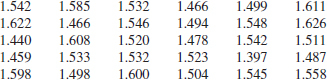
(a) Is there evidence to support the assumption that the tar content is normally distributed?
(b) Find a 99% CI on the mean tar content.
(c) Find a 99% prediction interval on the tar content for the next observation that will be taken on this particular type of tobacco.
(d) Find an interval that will contain 99% of the values of the tar content with 95% confidence.
(e) Explain the difference in the three intervals computed in parts (b), (c), and (d).
8-108. ![]() A manufacturer of electronic calculators takes a random sample of 1200 calculators and finds 8 defective units.
A manufacturer of electronic calculators takes a random sample of 1200 calculators and finds 8 defective units.
(a) Construct a 95% confidence interval on the population proportion.
(b) Is there evidence to support a claim that the fraction of defective units produced is 1% or less?
8-109. ![]() An article in The Engineer (“Redesign for Suspect Wiring,” June 1990) reported the results of an investigation into wiring errors on commercial transport aircraft that may display faulty information to the flight crew. Such a wiring error may have been responsible for the crash of a British Midland Airways aircraft in January 1989 by causing the pilot to shut down the wrong engine. Of 1600 randomly selected aircraft, 8 were found to have wiring errors that could display incorrect information to the flight crew.
An article in The Engineer (“Redesign for Suspect Wiring,” June 1990) reported the results of an investigation into wiring errors on commercial transport aircraft that may display faulty information to the flight crew. Such a wiring error may have been responsible for the crash of a British Midland Airways aircraft in January 1989 by causing the pilot to shut down the wrong engine. Of 1600 randomly selected aircraft, 8 were found to have wiring errors that could display incorrect information to the flight crew.
(a) Find a 99% confidence interval on the proportion of aircraft that have such wiring errors.
(b) Suppose that you use the information in this example to provide a preliminary estimate of p. How large a sample would be required to produce an estimate of p that we are 99% confident differs from the true value by at most 0.008?
(c) Suppose that you did not have a preliminary estimate of p. How large a sample would be required if you wanted to be at least 99% confident that the sample proportion differs from the true proportion by at most 0.008 regardless of the true value of p?
(d) Comment on the usefulness of preliminary information in computing the needed sample size.
8-110. ![]() An article in Engineering Horizons (Spring 1990, p. 26) reported that 117 of 484 new engineering graduates were planning to continue studying for an advanced degree. Consider this as a random sample of the 1990 graduating class.
An article in Engineering Horizons (Spring 1990, p. 26) reported that 117 of 484 new engineering graduates were planning to continue studying for an advanced degree. Consider this as a random sample of the 1990 graduating class.
(a) Find a 90% confidence interval on the proportion of such graduates planning to continue their education.
(b) Find a 95% confidence interval on the proportion of such graduates planning to continue their education.
(c) Compare your answers to parts (a) and (b) and explain why they are the same or different.
(d) Could you use either of these confidence intervals to determine whether the proportion is actually 0.25? Explain your answer. Hint: Use the normal approximation to the binomial.
8-111. An article in the Journal of Applied Physiology [“Humidity Does Not Affect Central Nervous System Oxygen Toxicity” (2001, Vol. 91, pp. 1327–1333)] reported that central nervous system (CNS) oxygen toxicity can appear in humans on exposure to oxygen pressures >180 kPa. CNS oxygen toxicity can occur as convulsions (similar to epileptic seizures, grand mal) and loss of consciousness without any warning symptoms. CNS oxygen toxicity is a risk encountered in several fields of human activity, such as combat diving with closed-circuit breathing apparatus and diving with mixtures of nitrogen and oxygen (nitrox) or nitrogen, oxygen, and helium (trimix) in sport and professional diving to depths >30 μ. The risk of oxygen toxicity is always considered when deep diving is planned. The following data demonstrate shortened latencies in a dry atmosphere (<10% humidity) in 11 rats at O2 of 507 kPa. The data collected are as follows:
![]()
(a) Given the following probability plot of the data, what is a logical assumption about the underlying distribution of the data?
(b) Explain why this check of the distribution underlying the sample data is important if you want to construct a confidence interval on the mean.
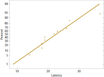
(c) Find the 95% confidence interval for the mean.
(d) Explain why this check of the distribution underlying the sample data is important if you want to construct a confidence interval on the variance.
(e) Find the 95% confidence interval for the variance.
8-112. An article in the Journal of Human Nutrition and Dietetics [“The Validation of Energy and Protein Intakes by Doubly Labeled Water and 24-Hour Urinary Nitrogen Excretion in Post-Obese Subjects” (1995, Vol. 8, pp. 51–64)] showed the energy intake expressed as a basal metabolic rate, BMR (MJ).
![]()
(a) Use a normal probability plot to check the normality assumption.
(b) Find a 99% two-sided confidence interval on the mean BMR.
Mind-Expanding Exercises
8-113. An electrical component has a time-to-failure (or lifetime) distribution that is exponential with parameter λ, so the mean lifetime is μ = 1/λ. Suppose that a sample of n of these components is put on test, and let Xi be the observed lifetime of component i. The test continues only until the rth unit fails, where r < n. This results in a censored life test. Let X1 denote the time at which the first failure occurred, X2 denote the time at which the second failure occurred, and so on. Then the total lifetime that has been accumulated at test termination is
![]()
We have previously shown in Exercise 7-81 that Tr/r is an unbiased estimator for μ.
(a) It can be shown that 2λTr has a chi-square distribution with 2r degrees of freedom. Use this fact to develop a 100(1 − α)% confidence interval for mean lifetime μ = 1/λ.
(b) Suppose that 20 units were tested, and the test terminated after 10 failures occurred. The failure times (in hours) are 15, 18, 19, 20, 21, 21, 22, 27, 28, and 29. Find a 95% confidence interval on mean lifetime.
8-114. Consider a two-sided confidence interval for the mean μ when σ is known:
![]()
where α1 + α2 = α. If α1 = α2 = α/2, you have the usual 100(1 − α)% confidence interval for μ. In the preceding, when α1 ≠ α2, the interval is not symmetric about μ. The length of the interval is L = σ(zα1 + zα2)/![]() . Prove that the length of the interval L is minimized when α1 = α2 = α/2. Hint: Remember that Φ(za) = 1 − α, so Φ − 1(1 − α) = zα, and the relationship between the derivative of a function y = f(x) and the inverse x = f −1(y) is (d/dy)f −1(y) = 1/[(d/dy)f(x)].
. Prove that the length of the interval L is minimized when α1 = α2 = α/2. Hint: Remember that Φ(za) = 1 − α, so Φ − 1(1 − α) = zα, and the relationship between the derivative of a function y = f(x) and the inverse x = f −1(y) is (d/dy)f −1(y) = 1/[(d/dy)f(x)].
8-115. It is possible to construct a nonparametric tolerance interval that is based on the extreme values in a random sample of size n from any continuous population. If p is the minimum proportion of the population contained between the smallest and largest sample observations with confidence 1 − α, it can be shown that
![]()
and n is approximately
![]()
(a) To be 95% confident that at least 90% of the population will be included between the extreme values of the sample, what sample size will be required?
(b) A random sample of 10 transistors gave the following measurements on saturation current (in milliamps): 10.25, 10.41, 10.30, 10.26, 10.19, 10.37, 10.29, 10.34, 10.23, 10.38. Find the limits that contain a proportion p of the saturation current measurements at 95% confidence. What is the proportion p contained by these limits?
8-116. Suppose that X1, X2, ..., Xn is a random sample from a continuous probability distribution with median ![]()
(a) Show that
![]()
[Hint: The complement of the event [min(Xi) < ![]() < max (Xi)] is [max (Xi) ≤
< max (Xi)] is [max (Xi) ≤ ![]() ] ∪ [min(Xi) ≤
] ∪ [min(Xi) ≤ ![]() ] but max (Xi) ≤
] but max (Xi) ≤ ![]() if and only if Xi ≤
if and only if Xi ≤ ![]() for all i.]
for all i.]
(b) Write down a 100(1 − α)% confidence interval for the median ![]() where
where
![]()
8-117. Students in the industrial statistics lab at ASU calculate confidence intervals on μ. Suppose that all these CIs are independent of each other. Consider the next one thousand 95% confidence intervals that will be calculated. How many of these CIs do you expect to capture the true value of μ? What is the probability that between 930 and 970 of these intervals contain the true value of μ?
8-118. The confidence interval for a population proportion depends on the central limit theorem. A common rule of thumb is that to use the normal approximation for the sampling distribution for ![]() , you should have at least 10 “successes” and 10 “failures.” However, Agresti and Coull developed a method that can be used for smaller samples and increases the accuracy of all confidence intervals for proportions. The idea is simply to add 4 “pseudo observations” to the data set—2 successes and 2 failures. That is, if you have X successes from of n trials, use
, you should have at least 10 “successes” and 10 “failures.” However, Agresti and Coull developed a method that can be used for smaller samples and increases the accuracy of all confidence intervals for proportions. The idea is simply to add 4 “pseudo observations” to the data set—2 successes and 2 failures. That is, if you have X successes from of n trials, use ![]() instead of the usual
instead of the usual ![]() in the formulas for the confidence interval.
in the formulas for the confidence interval.
A quality control engineer is inspecting defects on a newly designed printed circuit board. She inspects 50 boards and finds no defects. The usual estimate would be ![]() = 0, but she does not believe that there will ever be a no-defects situation for this product. Use this Agresi-Coull estimate to come up with a 95% confidence interval for the true proportion of defects. [Hint: The lower bound may be negative, which is not feasible, so simply use the upper limit and report that she is 95% confident that the true defect proportion is no higher than this number.]
= 0, but she does not believe that there will ever be a no-defects situation for this product. Use this Agresi-Coull estimate to come up with a 95% confidence interval for the true proportion of defects. [Hint: The lower bound may be negative, which is not feasible, so simply use the upper limit and report that she is 95% confident that the true defect proportion is no higher than this number.]
8-119. A biology student finds that of 35 males with Drosophila melanogaster, 2 have Adh genotypes with a male mating advantage.
(a) Using the standard methods, find a 95% confidence interval for the true proportion of males with this genotype.
(b) Compare the confidence interval you found in part (a) with the Agresti-Coull confidence interval by adding 4 pseudo-observations to the data discussed in the previous exercise.
Important Terms and Concepts
Chi-square distribution
Confidence coefficient
Confidence interval
Confidence interval for a population proportion
Confidence interval on the variance of a normal distribution
Confidence intervals on the mean of a normal distribution
Confidence level
Error in estimation
Large-sample confidence interval
One-sided confidence bounds
Prediction interval
Tolerance interval
Two-sided confidence interval
t distribution