

Joint Probability Distributions

Chapter Outline
5-1 Two or More Random Variables
5-1.1 Joint Probability Distributions
5-1.2 Marginal Probability Distributions
5-1.3 Conditional Probability Distributions
5-1.5 More Than Two Random Variables
5-2 Covariance and Correlation
5-3 Common Joint Distributions
5-3.1 Multinomial Probability Distribution
5-3.2 Bivariate Normal Distribution
5-4 Linear Functions of Random Variables
Air-quality monitoring stations are maintained throughout Maricopa County, Arizona and the Phoenix metropolitan area. Measurements for particulate matter and ozone are measured hourly. Particulate matter (known as PM10) is a measure (in μg/m3) of solid and liquid particles in the air with diameters less than 10 micrometers. Ozone is a colorless gas with molecules comprised of three oxygen atoms that make it very reactive. Ozone is formed in a complex reaction from heat, sunlight, and other pollutants, especially volatile organic compounds. The U.S. Environmental Protection Agency sets limits for both PM10 and ozone. For example, the limit for ozone is 0.075 ppm. The probability that a day in Phoenix exceeds the limits for PM10 and ozone is important for compliance and remedial actions with the county and city. But this might be more involved that the product of the probabilities for each pollutant separately. It might be that days with high PM10 measurements also tend to have ozone values. That is, the measurements might not be independent, so the joint relationship between these measurements becomes important. The study of probability distributions for more than one random variable is the focus of this chapter and the air-quality data is just one illustration of the ubiquitous need to study variables jointly.
After careful study of this chapter, you should be able to do the following:
- Use joint probability mass functions and joint probability density functions to calculate probabilities
- Calculate marginal and conditional probability distributions from joint probability distributions
- Interpret and calculate covariances and correlations between random variables
- Use the multinomial distribution to determine probabilities
- Understand properties of a bivariate normal distribution and be able to draw contour plots for the probability density function
- Calculate means and variances for linear combinations of random variables and calculate probabilities for linear combinations of normally distributed random variables
- Determine the distribution of a general function of a random variable
- Calculate moment generating functions and use the functions to determine moments and distributions
In Chapters 3 and 4, you studied probability distributions for a single random variable. However, it is often useful to have more than one random variable defined in a random experiment. For example, in the classification of transmitted and received signals, each signal can be classified as high, medium, or low quality. We might define the random variable X to be the number of high-quality signals received and the random variable Y to be the number of low-quality signals received. In another example, the continuous random variable X can denote the length of one dimension of an injection-molded part, and the continuous random variable Y might denote the length of another dimension. We might be interested in probabilities that can be expressed in terms of both X and Y. For example, if the specifications for X and Y are (2.95 to 3.05) and (7.60 to 7.80) millimeters, respectively, we might be interested in the probability that a part satisfies both specifications; that is, P(2.95 < X < 3.05 and 7.60 < Y < 7.80).
Because the two random variables are measurements from the same part, small disturbances in the injection-molding process, such as pressure and temperature variations, might be more likely to generate values for X and Y in specific regions of two-dimensional space. For example, a small pressure increase might generate parts such that both X and Y are greater than their respective targets, and a small pressure decrease might generate parts such that X and Y are both less than their respective targets. Therefore, based on pressure variations, we expect that the probability of a part with X much greater than its target and Y much less than its target is small.
In general, if X and Y are two random variables, the probability distribution that defines their simultaneous behavior is called a joint probability distribution. In this chapter, we investigate some important properties of these joint distributions.
5-1 Two or More Random Variables
5-1.1 JOINT PROBABILITY DISTRIBUTIONS
Joint Probability Mass Function
For simplicity, we begin by considering random experiments in which only two random variables are studied. In later sections, we generalize the presentation to the joint probability distribution of more than two random variables.
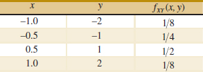
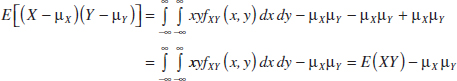
Example 5-1 Mobile Response Time The response time is the speed of page downloads and it is critical for a mobile Web site. As the response time increases, customers become more frustrated and potentially abandon the site for a competitive one. Let X denote the number of bars of service, and let Y denote the response time (to the nearest second) for a particular user and site.
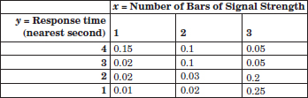
FIGURE 5-1 Joint probability distribution of X and Y in Example 5-1.
By specifying the probability of each of the points in Fig. 5-1, we specify the joint probability distribution of X and Y. Similarly to an individual random variable, we define the range of the random variables (X,Y) to be the set of points (x, y) in two-dimensional space for which the probability that X = x and Y = y is positive.
If X and Y are discrete random variables, the joint probability distribution of X and Y is a description of the set of points (x,y) in the range of (X,Y) along with the probability of each point. Also, P(X = x and Y = y) is usually written as P(X = x,Y = y). The joint probability distribution of two random variables is sometimes referred to as the bivariate probability distribution or bivariate distribution of the random variables. One way to describe the joint probability distribution of two discrete random variables is through a joint probability mass function f(x,y) = P(X = x,Y = y).
Joint Probability Mass Function
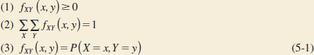
The joint probability mass function of the discrete random variables X and Y, denoted as fxy(x, y), satisfies
Just as the probability mass function of a single random variable X is assumed to be zero at all values outside the range of X, so the joint probability mass function of X and Y is assumed to be zero at values for which a probability is not specified.
Joint Probability Density Function
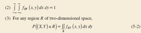
The joint probability distribution of two continuous random variables X and Y can be specified by providing a method for calculating the probability that X and Y assume a value in any region R of two-dimensional space. Analogous to the probability density function of a single continuous random variable, a joint probability density function can be defined over two-dimensional space. The double integral of fXY(x, y) over a region R provides the probability that (X,Y) assumes a value in R. This integral can be interpreted as the volume under the surface fXY(x, y) over the region R.
A joint probability density function for X and Y is shown in Fig. 5-2. The probability that (X,Y) assumes a value in the region R equals the volume of the shaded region in Fig. 5-2. In this manner, a joint probability density function is used to determine probabilities for X and Y.
Typically, fXY(x, y) is defined over all of two-dimensional space by assuming that fXY(x, y) = 0 for all points for which fXY(x, y) is not specified.
Joint Probability Density Function
A joint probability density function for the continuous random variables X and Y, denoted as fXY(x, y), satisfies the following properties:
![]()
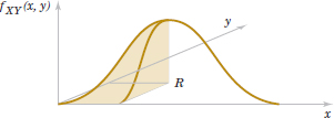
FIGURE 5-2 Joint probability density function for random variables X and Y. Probability that (X,Y) is in the region R is determined by the volume of fXY(x,y) over the region R.
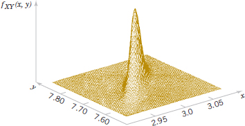
FIGURE 5-3 Joint probability density function for the lengths of different dimensions of an injection-molded part.
At the start of this chapter, the lengths of different dimensions of an injection-molded part were presented as an example of two random variables. However, because the measurements are from the same part, the random variables are typically not independent. If the specifications for X and Y are [2.95, 3.05] and [7.60, 7.80] millimeters, respectively, we might be interested in the probability that a part satisfies both specifications; that is, P(2.95 < X < 3.05, 7.60 < Y < 7.80). Suppose that fXY(x, y) is shown in Fig. 5-3. The required probability is the volume of fXY(x, y) within the specifications. Often a probability such as this must be determined from a numerical integration.
Example 5-2 Server Access Time Let the random variable X denote the time until a computer server connects to your machine (in milliseconds), and let Y denote the time until the server authorizes you as a valid user (in milliseconds). Each of these random variables measures the wait from a common starting time and X<Y. Assume that the joint probability density function for X and Y is
![]()
Reasonable assumptions can be used to develop such a distribution, but for now, our focus is on only the joint probability density function.
The region with nonzero probability is shaded in Fig. 5-4. The property that this joint probability density function integrates to 1 can be verified by the integral of fXY(x, y) over this region as follows:
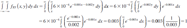
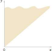
FIGURE 5-4 The joint probability density function of X and Y is nonzero over the shaded region.
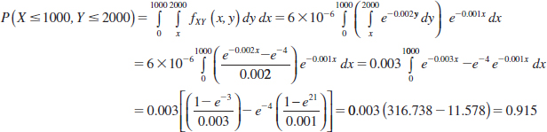
FIGURE 5-5 Region of integration for the probability that X<1000 and Y <2000 is darkly shaded.
The probability that X<1000 and Y<2000 is determined as the integral over the darkly shaded region in Fig. 5-5.
Practical Interpretation: A joint probability density function enables probabilities for two (or more) random variables to be calculated as in these examples.
5-1.2 MARGINAL PROBABILITY DISTRIBUTIONS
If more than one random variable is defined in a random experiment, it is important to distinguish between the joint probability distribution of X and Y and the probability distribution of each variable individually. The individual probability distribution of a random variable is referred to as its marginal probability distribution.
In general, the marginal probability distribution of X can be determined from the joint probability distribution of X and other random variables. For example, consider discrete random variables X and Y. To determine P(X = x), we sum P(X = x,Y = y) over all points in the range of (X,Y) for which X = x. Subscripts on the probability mass functions distinguish between the random variables.
Example 5-3 Marginal Distribution The joint probability distribution of X and Y in Fig. 5-1 can be used to find the marginal probability distribution of X. For example,
![]()
The marginal probability distribution for X is found by summing the probabilities in each column whereas the marginal probability distribution for Y is found by summing the probabilities in each row. The results are shown in Fig. 5-6.
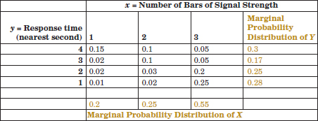
FIGURE 5-6 Marginal probability distributions of X and Y from Fig. 5-1.
For continuous random variables, an analogous approach is used to determine marginal probability distributions. In the continuous case, an integral replaces the sum.
Marginal Probability Density Function
If the joint probability density function of random variables X and Y is fXY(x, y), the marginal probability density functions of X and Y are
![]()
where the first integral is over all points in the range of (X,Y) for which X = x and the second integral over all points in the range of (X,Y) for which Y = y.
A probability for only one random variable, say, for example, P(a<X<b), can be found from the marginal probability distribution of X or from the integral of the joint probability distribution of X and Y as
![]()
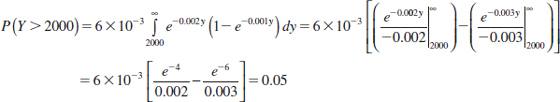
Example 5-4 Server Access Time For the random variables that denote times in Example 5-2, calculate the probability that Y exceeds 2000 milliseconds.
This probability is determined as the integral of fXY(x,y) over the darkly shaded region in Fig. 5-7. The region is partitioned into two parts and different limits of integration are determined for each part.
![]()
The first integral is

The second integral is


FIGURE 5-7 Region of integration for the probability that Y > 2000 is darkly shaded, and it is partitioned into two regions with x <2000 and x >2000.
Therefore,
![]()
Alternatively, the probability can be calculated from the marginal probability distribution of Y as follows. For y > 0,
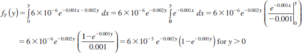
We have obtained the marginal probability density function of Y. Now,
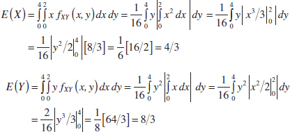
Also, E(X) and V(X) can be obtained by first calculating the marginal probability distribution of X and then determining E(X) and V(X) by the usual method. In Fig. 5-6, the marginal probability distributions of X and Y are used to obtain the means as
![]()
5-1.3 CONDITIONAL PROBABILITY DISTRIBUTIONS
When two random variables are defined in a random experiment, knowledge of one can change the probabilities that we associate with the values of the other. Recall that in Example 5-1, X denotes the number of bars of service and Y denotes the response time. One expects the probability Y = 1 to be greater at X = 3 bars than at X = 1 bar. From the notation for conditional probability in Chapter 2, we can write such conditional probabilities as P(Y = 1|X = 3) and P(Y = 1|X = 1). Consequently, the random variables X and Y are expected to be dependent. Knowledge of the value obtained for X changes the probabilities associated with the values of Y.
Recall that the definition of conditional probability for events A and B is P(B|A) = P(A ∩ B)/P(A). This definition can be applied with the event A defined to be X = x and event B defined to be Y = y.
Example 5-5 Conditional Probabilities for Mobile Response Time For Example 5-1, X and Y denote the number of bars of signal strength and response time, respectively. Then,
![]()
The probability that Y = 2 given that X = 3 is
![]()
Further work shows that
![]()
and
![]()
Note that P(Y = 1|X = 3) + P(Y = 2|X = 3) + P(Y = 3|X = 3) + P(Y = 4|X = 3) = 1. This set of probabilities defines the conditional probability distribution of Y given that X = 3.
Example 5-5 illustrates that the conditional probabilities for Y given that X = x can be thought of as a new probability distribution called the conditional probability mass function for Y given X = x. The following definition applies these concepts to continuous random variables.
Conditional Probability Density Function
Given continuous random variables X and Y with joint probability density function fXY(x,y), the conditional probability density function of Y given X = x is
![]()
The conditional probability density function provides the conditional probabilities for the values of Y given that X = x.
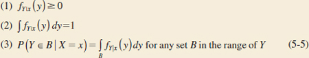
Because the conditional probability density function fY||x(y) is a probability density function for all y in Rx, the following properties are satisfied:
It is important to state the region in which a joint, marginal, or conditional probability density function is not zero. The following example illustrates this.
Example 5-6 Conditional Probability For the random variables that denote times in Example 5-2, determine the conditional probability density function for Y given that X = x.
First the marginal density function of x is determined. For x>0,
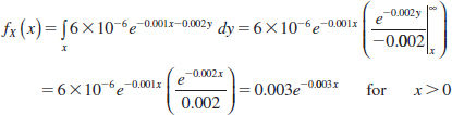
This is an exponential distribution with λ = 0.003. Now for 0 < x and x<y, the conditional probability density function is
![]()
The conditional probability density function of Y, given that X = 1500, is nonzero on the solid line in Fig. 5-8.
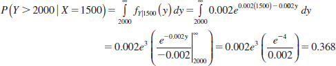
Determine the probability that Y exceeds 2000, given that x = 1500. That is, determine P(Y > 2000|X = 1500).
The conditional probability density function is integrated as follows:
Example 5-7 For the joint probability distribution in Fig. 5-1, fY|x(y) is found by dividing each fXY(x,y) by fx(x). Here, fx(x) is simply the sum of the probabilities in each column of Fig. 5-1. The function fY|x(y) is shown in Fig. 5-9. In Fig. 5-9, each column sums to 1 because it is a probability distribution.
Properties of random variables can be extended to a conditional probability distribution of Y given X = x. The usual formulas for mean and variance can be applied to a conditional probability density or mass function.
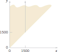
FIGURE 5-8 The conditional probability density function for Y, given that x = 1500, is nonzero over the solid line.
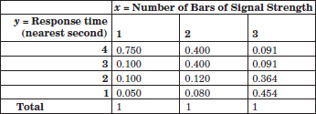
FIGURE 5-9 Conditional probability distributions of Y given X = x, fY|x (y) in Example 5-7.
Conditional Mean and Variance
The conditional mean of Y given X = x, denoted as E(Y|x) or μY|x, is
![]()
and the conditional variance of Y given X = x, denoted as V(Y|x) or ![]() , is
, is
![]()
Example 5-8 Conditional Mean And Variance For the random variables that denote times in Example 5-2, determine the conditional mean for Y given that x = 1500.
The conditional probability density function for Y was determined in Example 5-6. Because fY|1500(y) is nonzero for y > 1500,
![]()
Integrate by parts as follows:
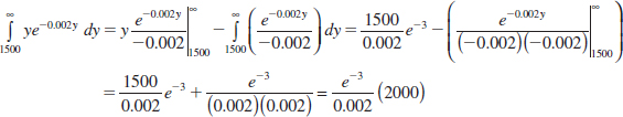
With the constant 0.002e3 reapplied,
![]()
Practical Interpretation: If the connect time is 1500 ms, then the expected time to be authorized is 2000 ms.
Example 5-9 For the discrete random variables in Example 5-1, the conditional mean of Y given X = 1 is obtained from the conditional distribution in Fig. 5-9:
![]()
The conditional mean is interpreted as the expected response time given that one bar of signal is present. The conditional variance of Y given X = 1 is
![]()
5-1.4 INDEPENDENCE
In some random experiments, knowledge of the values of X does not change any of the probabilities associated with the values for Y. In this case, marginal probability distributions can be used to calculate probabilities more easily.
Example 5-10 Independent Random Variables An orthopedic physician's practice considers the number of errors in a bill and the number of X-rays listed on the bill. There may or may not be a relationship between these random variables. Let the random variables X and Y denote the number of errors and the number of X-rays on a bill, respectively.
Assume that the joint probability distribution of X and Y is defined by fXY(x,y) in Fig. 5-10(a). The marginal probability distributions of X and Y are also shown in Fig. 5-10(a). Note that
![]()
The conditional probability mass function fY|x(y) is shown in Fig. 5-10(b). Notice that for any x, fY|x(y) = fY(y). That is, knowledge of whether or not the part meets color specifications does not change the probability that it meets length specifications.
By analogy with independent events, we define two random variables to be independent whenever fXY(x,y) = fX(x)fY(y) for all x and y. Notice that independence implies that fXY(x,y) = fX(x)fY(y) for all x and y. If we find one pair of x and y in which the equality fails, X and Y are not independent.
If two random variables are independent, then for fX(x)>0,
![]()
With similar calculations, the following equivalent statements can be shown.
Independence
For random variables X and Y, if any one of the following properties is true, the others are also true, and X and Y are independent.
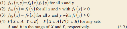
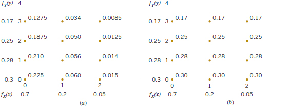
FIGURE 5-10 (a) Joint and marginal probability distributions of X and Y for Example 5-10. (b) Conditional probability distribution of Y given X = x for Example 5-10.
Rectangular Range for (X, Y)
Let D denote the set of points in two-dimensional space that receive positive probability under fXY(x,y). If D is not rectangular, X and Y are not independent because knowledge of X can restrict the range of values of Y that receive positive probability. If D is rectangular, independence is possible but not demonstrated. One of the conditions in Equation 5-6 must still be verified.
The variables in Example 5-2 are not independent. This can be quickly determined because the range of (X,Y) shown in Fig. 5-4 is not rectangular. Consequently, knowledge of X changes the interval of values for Y with nonzero probability.
Example 5-11 Independent Random Variables Suppose that Example 5-2 is modified so that the joint probability density function of X and Y is fXY(x,y) = 2×10⁻⁶exp(−0.001x −0.002y) for x ≥ 0 and y ≥ 0. Show that X and Y are independent and determine P(X > 1000, Y < 1000).
Note that the range of positive probability is rectangular so that independence is possible but not yet demonstrated. The marginal probability density function of X is
![]()
The marginal probability density function of Y is
![]()
Therefore, fXY(x,y) = fX(x)fY(y) for all x and y, and X and Y are independent.
To determine the probability requested, property (4) of Equation 5-7 can be applied along with the fact that each random variable has an exponential distribution. Therefore,
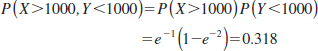
Often, based on knowledge of the system under study, random variables are assumed to be independent. Then probabilities involving both variables can be determined from the marginal probability distributions. For example, the time to complete a computer search should be independent of an adult's height.
Example 5-12 Machined Dimensions Let the random variables X and Y denote the lengths of two dimensions of a machined part, respectively. Assume that X and Y are independent random variables, and further assume that the distribution of X is normal with mean 10.5 millimeters and variance 0.0025 (mm2) and that the distribution of Y is normal with mean 3.2 millimeters and variance 0.0036 (mm2). Determine the probability that 10.4 < X<10.6 and 3.15 < Y<3.25.
Because X and Y are independent,
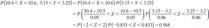
where Z denotes a standard normal random variable.
Practical Interpretation: If random variables are independent, probabilities for multiple variables are often much easier to compute.
5-1.5 MORE THAN TWO RANDOM VARIABLES
More than two random variables can be defined in a random experiment. Results for multiple random variables are straightforward extensions of those for two random variables. A summary is provided here.
Example 5-13 Machined Dimensions Many dimensions of a machined part are routinely measured during production. Let the random variables, X1, X2, X3, and X4 denote the lengths of four dimensions of a part. Then at least four random variables are of interest in this study.
The joint probability distribution of random variables X1, X2, X3,..., Xp can be specified with a method to calculate the probability that X1, X2, X3,..., Xp assume a value in any region R of p-dimensional space. For continuous random variables, a joint probability density function fX1X2...Xp(x1, x2,..., xp) is used to determine the probability that (X1, X2, X3,..., Xp) ∈ R by the multiple integral of fX1X2...Xp(x1, x2,..., xp) over the region R.
Joint Probability Density Function
A joint probability density function for the continuous random variables X1, X2, X3,..., Xp, denoted as fX1X2...Xp(x1, x2,..., xp), satisfies the following properties:
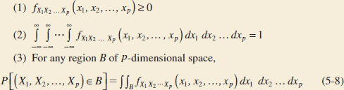
Typically, fX1X2...Xp(x1,x2,...,xp) is defined over all of p-dimensional space by assuming that fX1X2. . .Xp(x1,x2,..., xp) = 0 for all points for which fX1X2. . .Xp(x1,x2,...,xp) is not specified.
Example 5-14 Component Lifetimes In an electronic assembly, let the random variables X1, X2, X3, X4 denote the lifetime of four components, respectively, in hours. Suppose that the joint probability density function of these variables is
![]()
What is the probability that the device operates for more than 1000 hours without any failures? The requested probability is P(X1 > 1000, X2 > 1000, X3 > 1000, X4 > 1000), which equals the multiple integral of fX1X2X3X4(x1, x2, x3, x4) over the region x1 > 1000, x2 > 1000, x3 > 1000, x4 > 1000. The joint probability density function can be written as a product of exponential functions, and each integral is the simple integral of an exponential function. Therefore,
![]()
Suppose that the joint probability density function of several continuous random variables is a constant c over a region R (and zero elsewhere). In this special case,
![]()
by property (2) of Equation 5-8. Therefore, c = 1/(volume of region R). Furthermore, by property (3) of Equation 5-8, P[(X1, X2,..., Xp) ∈ B]
![]()
When the joint probability density function is constant, the probability that the random variables assume a value in the region B is just the ratio of the volume of the region B ∩ R to the volume of the region R for which the probability is positive.
Example 5-15 Probability as a Ratio of Volumes Suppose that the joint probability density function of the continuous random variables X and Y is constant over the region x2 + y2 ≤ 4. Determine the probability that X2 + Y2 ≤ 1.
The region that receives positive probability is a circle of radius 2. Therefore, the area of this region is 4π. The area of the region x2 + y2 ≤ 1 is π. Consequently, the requested probability is π/(4π) = 1/4.
Marginal Probability Density Function
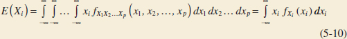
If the joint probability density function of continuous random variables X1, X2,..., Xp is fX1X2. . .Xp(x1, x2,..., xp), the marginal probability density function of Xi is
![]()
where the integral is over all points in the range of X1, X2,..., Xp for which Xi = xi.
As for two random variables, a probability involving only one random variable, for example, P(a < Xi < b), can be determined from the marginal probability distribution of Xi or from the joint probability distribution of X1, X2,..., Xp. That is,
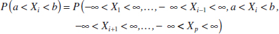
Furthermore, E(Xi) and V(Xi) for i = 1, 2,..., p can be determined from the marginal probability distribution of Xi or from the joint probability distribution of X1, X2,..., Xp as follows.
Mean and Variance from Joint Distribution
and
![]()
Example 5-16 Points that have positive probability in the joint probability distribution of three random variables X1, X2, X3 are shown in Fig. 5-11. Suppose the 10 points are equally likely with probability 0.1 each. The range is the non-negative integers with x1 + x2 + x3 = 3. The marginal probability distribution of X2 is found as follows.
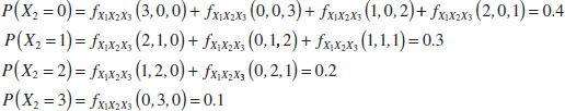
Also, E(X2) = 0(0.4)+1(0.3)+2(0.2)+3(0.1) = 1
With several random variables, we might be interested in the probability distribution of some subset of the collection of variables. The probability distribution of X1, X2,..., Xk, k < p can be obtained from the joint probability distribution of X1, X2,..., Xp as follows.
Distribution of a Subset of Random Variables
If the joint probability density function of continuous random variables X1, X2,..., Xp is fX1X2. . .Xp(x1, x2,..., xp), the probability density function of X1, X2,..., Xk, k<p, is
![]()
where the integral is over all points R in the range of X1, X2,..., Xp for which X1 = x1, X2 = x2,..., Xk = xk.
Conditional Probability Distribution
Conditional probability distributions can be developed for multiple random variables by an extension of the ideas used for two random variables. For example, the joint conditional probability distribution of X1, X2, and X3 given (X4 = x4, X5 = x5) is
![]()
The concept of independence can be extended to multiple random variables.
Independence
Random variables X1, X2,..., Xp are independent if and only if
![]()
Similar to the result for only two random variables, independence implies that Equation 5-12 holds for all x1, x2,..., xp. If we find one point for which the equality fails, X1, X2,..., Xp are not independent. It is left as an exercise to show that if X1, X2,..., Xp are independent,
![]()
for any regions A1, A2,..., Ap in the range of X1, X2,..., Xp, respectively.
Example 5-17 In Chapter 3, we showed that a negative binomial random variable with parameters p and r can be represented as a sum of r geometric random variables X1, X2,..., Xr. Each geometric random variable represents the additional trials required to obtain the next success. Because the trials in a binomial experiment are independent, X1, X2,..., Xr are independent random variables.
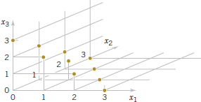
FIGURE 5-11 Joint probability distribution of X1, X2, and X3. Points are equally likely.
Example 5-18 Layer Thickness Suppose that X1, X2, and X3 represent the thickness in micrometers of a substrate, an active layer, and a coating layer of a chemical product, respectively. Assume that X1, X2, and X3 are independent and normally distributed with μ1 = 10000, μ2 = 1000, μ3 = 80, σ1 = 250, σ2 = 20, and σ3 = 4, respectively. The specifications for the thickness of the substrate, active layer, and coating layer are 9200 < x1 < 10,800,950 < x2 < 1050, and 75 < x3 < 85, respectively. What proportion of chemical products meets all thickness specifications? Which one of the three thicknesses has the least probability of meeting specifications?
The requested probability is P(9200<X1<10,800, 950<X2<1050, 75<X3<85). Because the random variables are independent,
![]()
After standardizing, the above equals
![]()
where Z is a standard normal random variable. From the table of the standard normal distribution, the requested probability equals
![]()
The thickness of the coating layer has the least probability of meeting specifications. Consequently, a priority should be to reduce variability in this part of the process.
EXERCISES FOR SECTION 5-1
![]() Problem available in WileyPLUS at instructor's discretion.
Problem available in WileyPLUS at instructor's discretion.
![]() Go Tutorial Tutoring problem available in WileyPLUS at instructor's discretion.
Go Tutorial Tutoring problem available in WileyPLUS at instructor's discretion.
5-1. ![]() Show that the following function satisfies the properties of a joint probability mass function.
Show that the following function satisfies the properties of a joint probability mass function.
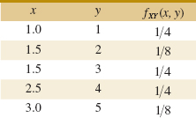
Determine the following:
(a) P(X < 2.5, Y < 3)
(b) P(X < 2.5)
(c) P(Y < 3)
(d) P(X > 1.8, Y > 4.7)
(e) E(X), E(Y), V(X), and V(Y).
(f) Marginal probability distribution of X
(g) Conditional probability distribution of Y given that X = 1.5
(h) Conditional probability distribution of X given that Y = 2
(i) E(Y|X = 1.5)
(j) Are X and Y independent?
5-2. ![]() Determine the value of c that makes the function f(x,y) = c(x+y) a joint probability mass function over the nine points with x = 1,2,3 and y = 1,2,3.
Determine the value of c that makes the function f(x,y) = c(x+y) a joint probability mass function over the nine points with x = 1,2,3 and y = 1,2,3.
Determine the following:
(a) P(X = 1, Y < 4)
(b) P(X = 1)
(c) P(Y = 2)
(d) P(X < 2, Y < 2)
(e) E(X), E(Y), V(X), and V(Y)
(f) Marginal probability distribution of X
(g) Conditional probability distribution of Y given that X = 1
(h) Conditional probability distribution of X given that Y = 2
(i) E(Y|X = 1)
(j) Are X and Y independent?
5-3. ![]() Show that the following function satisfies the properties of a joint probability mass function.
Show that the following function satisfies the properties of a joint probability mass function.
Determine the following:
(a) P(X < 0.5, Y < 1.5)
(b) P(X < 0.5)
(c) P(Y < 1.5)
(d) P(X > 0.25, Y < 4.5)
(e) E(X), E(Y), V(X), and V(Y)
(f) Marginal probability distribution of X
(g) Conditional probability distribution of Y given that X = 1
(h) Conditional probability distribution of X given that Y = 1
(i) E(X|y = 1)
(j) Are X and Y independent?
5-4. ![]() Four electronic printers are selected from a large lot of damaged printers. Each printer is inspected and classified as containing either a major or a minor defect. Let the random variables X and Y denote the number of printers with major and minor defects, respectively. Determine the range of the joint probability distribution of X and Y.
Four electronic printers are selected from a large lot of damaged printers. Each printer is inspected and classified as containing either a major or a minor defect. Let the random variables X and Y denote the number of printers with major and minor defects, respectively. Determine the range of the joint probability distribution of X and Y.
5-5. ![]() In the transmission of digital information, the probability that a bit has high, moderate, and low distortion is 0.01, 0.04, and 0.95, respectively. Suppose that three bits are transmitted and that the amount of distortion of each bit is assumed to be independent. Let X and Y denote the number of bits with high and moderate distortion out of the three, respectively. Determine:
In the transmission of digital information, the probability that a bit has high, moderate, and low distortion is 0.01, 0.04, and 0.95, respectively. Suppose that three bits are transmitted and that the amount of distortion of each bit is assumed to be independent. Let X and Y denote the number of bits with high and moderate distortion out of the three, respectively. Determine:
(a) fXY(x, y)
(b) fX(x)
(c) E(X)
(d) fY|1(y)
(e) E(Y|X = 1)
(f) Are X and Y independent?
5-6. ![]() A small-business Web site contains 100 pages and 60%, 30%, and 10% of the pages contain low, moderate, and high graphic content, respectively. A sample of four pages is selected without replacement, and X and Y denote the number of pages with moderate and high graphics output in the sample. Determine:
A small-business Web site contains 100 pages and 60%, 30%, and 10% of the pages contain low, moderate, and high graphic content, respectively. A sample of four pages is selected without replacement, and X and Y denote the number of pages with moderate and high graphics output in the sample. Determine:
(a) fXY(x, y)
(b) fX(x)
(c) E(X)
(d) fY|3(y)
(e) E(Y|X = 3)
(f) V(Y|X = 3)
(g) Are X and Y independent?
5-7. ![]() A manufacturing company employs two devices to inspect output for quality control purposes. The first device is able to accurately detect 99.3% of the defective items it receives, whereas the second is able to do so in 99.7% of the cases. Assume that four defective items are produced and sent out for inspection. Let X and Y denote the number of items that will be identified as defective by inspecting devices 1 and 2, respectively. Assume that the devices are independent. Determine:
A manufacturing company employs two devices to inspect output for quality control purposes. The first device is able to accurately detect 99.3% of the defective items it receives, whereas the second is able to do so in 99.7% of the cases. Assume that four defective items are produced and sent out for inspection. Let X and Y denote the number of items that will be identified as defective by inspecting devices 1 and 2, respectively. Assume that the devices are independent. Determine:
(a) fXY(x, y)
(b) fX(x)
(c) E(X)
(d) fY|2 (y)
(e) E(Y|X = 2)
(f) V(Y|X = 2)
(g) Are X and Y independent?
5-8. ![]() Suppose that the random variables X, Y, and Z have the following joint probability distribution.
Suppose that the random variables X, Y, and Z have the following joint probability distribution.
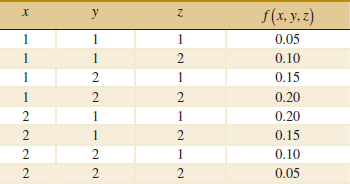
Determine the following:
(a) P(X = 2)
(b) P(X = 1, Y = 2)
(c) P(Z < 1.5)
(d) P(X = 1 or Z = 2)
(e) E(X)
(f) P(X = 1|Y = 1)
(g) P(X = 1, Y = 1|Z = 2)
(h) P(X = 1|Y = 1, Z = 2)
(i) Conditional probability distribution of X given that Y = 1 and Z = 2
5-9. An engineering statistics class has 40 students; 60% are electrical engineering majors, 10% are industrial engineering majors, and 30% are mechanical engineering majors. A sample of four students is selected randomly without replacement for a project team. Let X and Y denote the number of industrial engineering and mechanical engineering majors, respectively. Determine the following:
(a) fXY(x, y)
(b) fX(x)
(c) E(X)
(d) fY|3(y)
(e) E(Y|X = 3)
(f) V(Y|X = 3)
(g) Are X and Y independent?
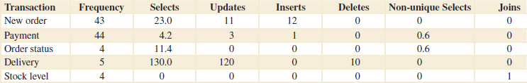
5-10. ![]() An article in the Journal of Database Management [“Experimental Study of a Self-Tuning Algorithm for DBMS Buffer Pools” (2005, Vol. 16, pp. 1–20)] provided the workload used in the TPC-C OLTP (Transaction Processing Performance Council's Version C On-Line Transaction Processing) benchmark, which simulates a typical order entry application. See the following table. The frequency of each type of transaction (in the second column) can be used as the percentage of each type of transaction. Let X and Y denote the average number of selects and updates operations, respectively, required for each type transaction. Determine the following:
An article in the Journal of Database Management [“Experimental Study of a Self-Tuning Algorithm for DBMS Buffer Pools” (2005, Vol. 16, pp. 1–20)] provided the workload used in the TPC-C OLTP (Transaction Processing Performance Council's Version C On-Line Transaction Processing) benchmark, which simulates a typical order entry application. See the following table. The frequency of each type of transaction (in the second column) can be used as the percentage of each type of transaction. Let X and Y denote the average number of selects and updates operations, respectively, required for each type transaction. Determine the following:
(a) P(X < 5)
(b) E(X)
(c) Conditional probability mass function of X given Y = 0
(d) P(X < 6|Y = 0)
(e) E(X|Y = 0)
5-11. ![]() For the Transaction Processing Performance Council's benchmark in Exercise 5-10, let X, Y, and Z denote the average number of selects, updates, and inserts operations required for each type of transaction, respectively. Calculate the following:
For the Transaction Processing Performance Council's benchmark in Exercise 5-10, let X, Y, and Z denote the average number of selects, updates, and inserts operations required for each type of transaction, respectively. Calculate the following:
(a) fXYZ(x, y, z)
(b) Conditional probability mass function for X and Y given Z = 0
(c) P(X < 6, Y < 6|Z = 0)
(d) E(X|Y = 0, Z = 0)
5-12. ![]() In the transmission of digital information, the probability that a bit has high, moderate, or low distortion is 0.01, 0.04, and 0.95, respectively. Suppose that three bits are transmitted and that the amount of distortion of each bit is assumed to be independent. Let X and Y denote the number of bits with high and moderate distortion of the three transmitted, respectively. Determine the following:
In the transmission of digital information, the probability that a bit has high, moderate, or low distortion is 0.01, 0.04, and 0.95, respectively. Suppose that three bits are transmitted and that the amount of distortion of each bit is assumed to be independent. Let X and Y denote the number of bits with high and moderate distortion of the three transmitted, respectively. Determine the following:
Average Frequencies and Operations in TPC-C
(a) Probability that two bits have high distortion and one has moderate distortion
(b) Probability that all three bits have low distortion
(c) Probability distribution, mean, and variance of X
(d) Conditional probability distribution, conditional mean, and conditional variance of X given that Y = 2
5-13. ![]() Determine the value of c such that the function f(x,y) = cxy for 0 < x < 3 and 0 < y < 3 satisfies the properties of a joint probability density function.
Determine the value of c such that the function f(x,y) = cxy for 0 < x < 3 and 0 < y < 3 satisfies the properties of a joint probability density function.
Determine the following:
(a) P(X < 2, Y < 3)
(b) P(X < 2.5)
(c) P(1 < Y < 2.5)
(d) P(X > 1.8, 1 < Y < 2.5)
(e) E(X)
(f) P(X < 0, Y < 4)
(g) Marginal probability distribution of X
(h) Conditional probability distribution of Y given that X = 1.5
(i) E(Y|X) = 1.5)
(j) P(Y < 2|X = 1.5)
(k) Conditional probability distribution of X given that Y = 2
5-14. ![]() Determine the value of c that makes the function f(x, y) = c(x + y) a joint probability density function over the range 0 < x < 3 and x < y < x + 2.
Determine the value of c that makes the function f(x, y) = c(x + y) a joint probability density function over the range 0 < x < 3 and x < y < x + 2.
Determine the following:
(a) P(X < 1, Y < 2)
(b) P(1 < X < 2)
(c) P(Y > 1)
(d) P(X < 2, Y < 2)
(e) E(X)
(f) V(X)
(g) Marginal probability distribution of X
(h) Conditional probability distribution of Y given that X = 1
(i) E(Y|X = 1)
(j) P(Y > 2|X = 1)
(k) Conditional probability distribution of X given that Y = 2
5-15. ![]() Determine the value of c that makes the function f(x,y) = c(x + y) a joint probability density function over the range 0 < x<3 and 0 < y<x.
Determine the value of c that makes the function f(x,y) = c(x + y) a joint probability density function over the range 0 < x<3 and 0 < y<x.
Determine the following:
(a) P(X < 1,Y < 2)
(b) P(1 < X < 2)
(c) P(Y > 1)
(d) P(X < 2, Y < 2)
(e) E(X)
(f) E(Y)
(g) Marginal probability distribution of X
(h) Conditional probability distribution of Y given X = 1
(i) E(Y|X = 1)
(j) P(Y > 2|X = 1)
(k) Conditional probability distribution of X given Y = 2
5-16. ![]() Determine the value of c that makes the function f(x, y) = ce− 2x −3y a joint probability density function over the range 0 < x and 0 < y<x.
Determine the value of c that makes the function f(x, y) = ce− 2x −3y a joint probability density function over the range 0 < x and 0 < y<x.
Determine the following:
(a) P(X < 1, Y < 2)
(b) P(1 < X < 2)
(c) P(Y > 3)
(d) P(X < 2, Y < 2)
(e) E(X)
(f) E(Y)
(g) Marginal probability distribution of X
(h) Conditional probability distribution of Y given X = 1
(i) E(Y|X = 1)
(j) Conditional probability distribution of X given Y = 2
5-17. Determine the value of c that makes the function f(x,y) = ce−2x−3y, a joint probability density function over the range 0 < x and x<y.
Determine the following:
(a) P(X < 1, Y < 2)
(b) P(1 < X < 2)
(c) P(Y > 3)
(d) P(X < 2, Y < 2)
(e) E(X)
(f) E(Y)
(g) Marginal probability distribution of X
(h) Conditional probability distribution of Y given X = 1
(i) E(Y|X = 1)
(j) P(Y < 2|X = 1)
(k) Conditional probability distribution of X given Y = 2
5-18. The conditional probability distribution of Y given X = x is fY|x(y) = xe−xy for y > 0, and the marginal probability distribution of X is a continuous uniform distribution over 0 to 10.
(a) Graph fY|x(y) = xe−xy for y > 0 for several values of x.
Determine:
(b) P(Y < 2|X = 2)
(c) E(Y|X = 2)
(d) E(Y|X = x)
(e) fXY(x, y)
(f) fY(y)
5-19. Two methods of measuring surface smoothness are used to evaluate a paper product. The measurements are recorded as deviations from the nominal surface smoothness in coded units. The joint probability distribution of the two measurements is a uniform distribution over the region 0 < x < 4, 0 < y, and x − 1 < y < x + 1. That is, fXY(x, y) = c for x and y in the region. Determine the value for c such that fXY(x, y) is a joint probability density function.
Determine the following:
(a) P(X < 0.5, Y < 0.5)
(b) P(X < 0.5)
(c) E(X)
(d) E(Y)
(e) Marginal probability distribution of X
(f) Conditional probability distribution of Y given X = 1
(g) E(Y|X = 1)
(h) P(Y < 0.5|X = 1)
5-20. ![]() The time between surface finish problems in a galvanizing process is exponentially distributed with a mean of 40 hours. A single plant operates three galvanizing lines that are assumed to operate independently.
The time between surface finish problems in a galvanizing process is exponentially distributed with a mean of 40 hours. A single plant operates three galvanizing lines that are assumed to operate independently.
(a) What is the probability that none of the lines experiences a surface finish problem in 40 hours of operation?
(b) What is the probability that all three lines experience a surface finish problem between 20 and 40 hours of operation?
(c) Why is the joint probability density function not needed to answer the previous questions?
5-21. ![]() A popular clothing manufacturer receives Internet orders via two different routing systems. The time between orders for each routing system in a typical day is known to be exponentially distributed with a mean of 3.2 minutes. Both systems operate independently.
A popular clothing manufacturer receives Internet orders via two different routing systems. The time between orders for each routing system in a typical day is known to be exponentially distributed with a mean of 3.2 minutes. Both systems operate independently.
(a) What is the probability that no orders will be received in a 5-minute period? In a 10-minute period?
(b) What is the probability that both systems receive two orders between 10 and 15 minutes after the site is officially open for business?
(c) Why is the joint probability distribution not needed to answer the previous questions?
5-22. ![]() The blade and the bearings are important parts of a lathe. The lathe can operate only when both of them work properly. The lifetime of the blade is exponentially distributed with the mean three years; the lifetime of the bearings is also exponentially distributed with the mean four years. Assume that each lifetime is independent.
The blade and the bearings are important parts of a lathe. The lathe can operate only when both of them work properly. The lifetime of the blade is exponentially distributed with the mean three years; the lifetime of the bearings is also exponentially distributed with the mean four years. Assume that each lifetime is independent.
(a) What is the probability that the lathe will operate for at least five years?
(b) The lifetime of the lathe exceeds what time with 95% probability?
5-23. ![]() Suppose that the random variables X, Y, and Z have the joint probability density function f(x, y, z) = 8xyz for 0 < x<1, 0 < y<1, and 0 < z<1. Determine the following:
Suppose that the random variables X, Y, and Z have the joint probability density function f(x, y, z) = 8xyz for 0 < x<1, 0 < y<1, and 0 < z<1. Determine the following:
(a) P(X < 0.5)
(b) P(X < 0.5, Y < 0.5)
(c) P(Z < 2)
(d) P(X < 0.5 or Z < 2)
(e) E(X)
(f) P(X < 0.5|Y = 0.5)
(g) P(X < 0.5, Y < 0.5|Z = 0.8)
(h) Conditional probability distribution of X given that Y = 0.5 and Z = 0.8
(i) P(X < 0.5|Y = 0.5, Z = 0.8)
5-24. Suppose that the random variables X, Y, and Z have the joint probability density function fXYZ(x, y, z) = c over the cylinder x2 + y2 < 4 and 0 < z < 4. Determine the constant c so that fXYZ(x, y, z) is a probability density function.
Determine the following:
(a) P(X2 + Y2 < 2)
(b) P(Z < 2)
(c) E(X)
(d) P(X < 1|Y = 1)
(e) P(X2 + Y2 < 1|Z = 1)
(f) Conditional probability distribution of Z given that X = 1 and Y = 1.
5-25. Determine the value of c that makes fXYZ(x, y, z) = c a joint probability density function over the region x > 0, y > 0, z > 0, and x + y + z < 1.
Determine the following:
(a) P(X < 0.5, Y < 0.5, Z < 0.5)
(b) P(X < 0.5, Y < 0.5)
(c) P(X < 0.5)
(d) E(X)
(e) Marginal distribution of X
(f) Joint distribution of X and Y
(g) Conditional probability distribution of X given that Y = 0.5 and Z = 0.5
(h) Conditional probability distribution of X given that Y = 0.5
5-26. ![]() The yield in pounds from a day's production is normally distributed with a mean of 1500 pounds and standard deviation of 100 pounds. Assume that the yields on different days are independent random variables.
The yield in pounds from a day's production is normally distributed with a mean of 1500 pounds and standard deviation of 100 pounds. Assume that the yields on different days are independent random variables.
(a) What is the probability that the production yield exceeds 1400 pounds on each of five days next week?
(b) What is the probability that the production yield exceeds 1400 pounds on at least four of the five days next week?
5-27. ![]() The weights of adobe bricks used for construction are normally distributed with a mean of 3 pounds and a standard deviation of 0.25 pound. Assume that the weights of the bricks are independent and that a random sample of 20 bricks is selected.
The weights of adobe bricks used for construction are normally distributed with a mean of 3 pounds and a standard deviation of 0.25 pound. Assume that the weights of the bricks are independent and that a random sample of 20 bricks is selected.
(a) What is the probability that all the bricks in the sample exceed 2.75 pounds?
(b) What is the probability that the heaviest brick in the sample exceeds 3.75 pounds?
5-28. ![]() A manufacturer of electroluminescent lamps knows that the amount of luminescent ink deposited on one of its products is normally distributed with a mean of 1.2 grams and a standard deviation of 0.03 gram. Any lamp with less than 1.14 grams of luminescent ink fails to meet customers' specifications. A random sample of 25 lamps is collected and the mass of luminescent ink on each is measured.
A manufacturer of electroluminescent lamps knows that the amount of luminescent ink deposited on one of its products is normally distributed with a mean of 1.2 grams and a standard deviation of 0.03 gram. Any lamp with less than 1.14 grams of luminescent ink fails to meet customers' specifications. A random sample of 25 lamps is collected and the mass of luminescent ink on each is measured.
(a) What is the probability that at least one lamp fails to meet specifications?
(b) What is the probability that five or fewer lamps fail to meet specifications?
(c) What is the probability that all lamps conform to specifications?
(d) Why is the joint probability distribution of the 25 lamps not needed to answer the previous questions?
5-29. The lengths of the minor and major axes are used to summarize dust particles that are approximately elliptical in shape. Let X and Y denote the lengths of the minor and major axes (in micrometers), respectively. Suppose that fX(x) = exp(−x), 0 < x and the conditional distribution fY|x(y) = exp[−(y−x)], x < y. Answer or determine the following:
(a) That fY|x(y) is a probability density function for any value of x.
(b) P(X < Y) and comment on the magnitudes of X and Y.
(c) Joint probability density function fXY(x, y).
(d) Conditional probability density function of X given Y = y.
(e) P(Y < 2|X = 1)
(f) E(Y|X = 1)
(g) P(X < 1, Y < 1)
(h) P(Y < 2)
(i) c such that P(Y < c) = 0.9
(j) Are X and Y independent?
5-30. An article in Health Economics [“Estimation of the Transition Matrix of a Discrete-Time Markov Chain” (2002, Vol.11, pp. 33–42)] considered the changes in CD4 white blood cell counts from one month to the next. The CD4 count is an important clinical measure to determine the severity of HIV infections. The CD4 count was grouped into three distinct categories: 0–49, 50–74, and ≥ 75. Let X and Y denote the (category minimum) CD4 count at a month and the following month, respectively. The conditional probabilities for Y given values for X were provided by a transition probability matrix shown in the following table.
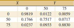
This table is interpreted as follows. For example, P(Y = 50|X = 75) = 0.0717. Suppose also that the probability distribution for X is P(X = 75) = 0.9,P(X = 50) = 0.08,P(X = 0) = 0.02. Determine the following:
(a) P(Y ≤ 50|X = 50)
(b) P(X = 0, Y = 75)
(c) E(Y|X = 50)
(d) fY(y)
(e) fXY(x, y)
(f) Are X and Y independent?
5-31. An article in Clinical Infectious Diseases [“Strengthening the Supply of Routinely Administered Vaccines in the United States: Problems and Proposed Solutions” (2006, Vol.42(3), pp. S97–S103)] reported that recommended vaccines for infants and children were periodically unavailable or in short supply in the United States. Although the number of doses demanded each month is a discrete random variable, the large demands can be approximated with a continuous probability distribution. Suppose that the monthly demands for two of those vaccines, namely measles–mumps–rubella (MMR) and varicella (for chickenpox), are independently, normally distributed with means of 1.1 and 0.55 million doses and standard deviations of 0.3 and 0.1 million doses, respectively. Also suppose that the inventory levels at the beginning of a given month for MMR and varicella vaccines are 1.2 and 0.6 million doses, respectively.
(a) What is the probability that there is no shortage of either vaccine in a month without any vaccine production?
(b) To what should inventory levels be set so that the probability is 90% that there is no shortage of either vaccine in a month without production? Can there be more than one answer? Explain.
5-32. The systolic and diastolic blood pressure values (mm Hg) are the pressures when the heart muscle contracts and relaxes (denoted as Y and X, respectively). Over a collection of individuals, the distribution of diastolic pressure is normal with mean 73 and standard deviation 8. The systolic pressure is conditionally normally distributed with mean 1.6x when X = x and standard deviation of 10. Determine the following:
(a) Conditional probability density function fY|73(y) of Y given X = 73
(b) P(Y < 115|X = 73)
(c) E(Y|X = 73)
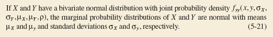
(d) Recognize the distribution fXY(x, y) and identify the mean and variance of Y and the correlation between X and Y
5-2 Covariance and Correlation
When two or more random variables are defined on a probability space, it is useful to describe how they vary together; that is, it is useful to measure the relationship between the variables. A common measure of the relationship between two random variables is the covariance. To define the covariance, we need to describe the expected value of a function of two random variables h(X, Y). The definition simply extends the one for a function of a single random variable.
Expected Value of a Function of Two Random Variables
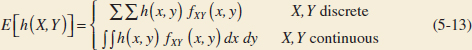
That is, E[h(X, Y)] can be thought of as the weighted average of h(x, y) for each point in the range of (X, Y). The value of E[h(X, Y)] represents the average value of h(X, Y) that is expected in a long sequence of repeated trials of the random experiment.
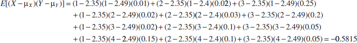
Example 5-19 Expected Value of a Function of Two Random Variables For the joint probability distribution of the two random variables in Example 5-1, calculate E[(X − μX)(Y − μY)].
The result is obtained by multiplying x − μX times y − μY, times fxy(X, Y) for each point in the range of (X, Y). First, μX and μY were determined previously from the marginal distributions for X and Y:
![]()
and
![]()
Therefore,
The covariance is defined for both continuous and discrete random variables by the same formula.
The covariance between the random variables X and Y, denoted as cov(X, Y) or σXY, is
![]()
If the points in the joint probability distribution of X and Y that receive positive probability tend to fall along a line of positive (or negative) slope, σXY, is positive (or negative). If the points tend to fall along a line of positive slope, X tends to be greater than μX when Y is greater than μY. Therefore, the product of the two terms x − μX and y − μY tends to be positive. However, if the points tend to fall along a line of negative slope, x − μX tends to be positive when y − μY is negative, and vice versa. Therefore, the product of x − μX and y − μY tends to be negative. In this sense, the covariance between X and Y describes the variation between the two random variables. Figure 5-12 assumes all points are equally likely and shows examples of pairs of random variables with positive, negative, and zero covariance.
Covariance is a measure of linear relationship between the random variables. If the relationship between the random variables is nonlinear, the covariance might not be sensitive to the relationship. This is illustrated in Fig. 5-12(d). The only points with nonzero probability are the points on the circle. There is an identifiable relationship between the variables. Still, the covariance is zero.
The equality of the two expressions for covariance in Equation 5-14 is shown for continuous random variables as follows. By writing the expectations as integrals,
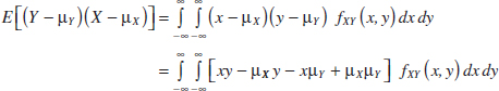
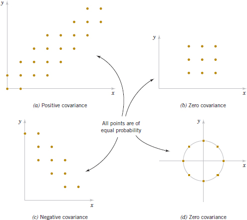
FIGURE 5-12 Joint probability distributions and the sign of covariance between X and Y.
![]()
Therefore,
Example 5-20 In Example 5-1, the random variables X and Y are the number of signal bars and the response time (to the nearest second), respectively. Interpret the covariance between X and Y as positive or negative.
As the signal bars increase, the response time tends to decrease. Therefore, X and Y have a negative covariance. The covariance was calculated to be −0.5815 in Example 5-19.
There is another measure of the relationship between two random variables that is often easier to interpret than the covariance.
Correlation
The correlation between random variables X and Y, denoted as ρXY, is
![]()
Because σX > 0 and σY > 0, if the covariance between X and Y is positive, negative, or zero, the correlation between X and Y is positive, negative, or zero, respectively. The following result can be shown.
For any two random variables X and Y,
![]()
The correlation just scales the covariance by the product of the standard deviation of each variable. Consequently, the correlation is a dimensionless quantity that can be used to compare the linear relationships between pairs of variables in different units.
If the points in the joint probability distribution of X and Y that receive positive probability tend to fall along a line of positive (or negative) slope, ρXY is near + 1 (or −1). If ρXY equals +1 or −1, it can be shown that the points in the joint probability distribution that receive positive probability fall exactly along a straight line. Two random variables with nonzero correlation are said to be correlated. Similar to covariance, the correlation is a measure of the linear relationship between random variables.
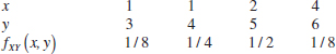
Example 5-21 Covariance For the discrete random variables X and Y with the joint distribution shown in Fig. 5-13, determine σXY and ρXY.
The calculations for E(XY), E(X), and V(X) are as follows.
![]()

Because the marginal probability distribution of Y is the same as for X, E(Y) = 1.8 and V(Y) = 1.36. Consequently,
![]()
Furthermore,
![]()
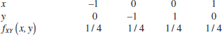
Example 5-22 Correlation Suppose that the random variable X has the following distribution: P(X = 1) = 0.2, P(X = 2) = 0.6, P(X = 3) = 0.2. Let Y = 2X + 5. That is, P(Y = 7) = 0.2, P(Y = 11) = 0.2. Determine the correlation between X and Y. Refer to Fig. 5-14.
Because X and Y are linearly related, ρ = 1. This can be verified by direct calculations: Try it.
For independent random variables, we do not expect any relationship in their joint probability distribution. The following result is left as an exercise.
If X and Y are independent random variables,
![]()
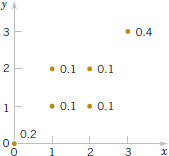
FIGURE 5-13 Joint distribution for Example 5-20.
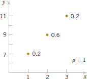
FIGURE 5-14 Joint distribution for Example 5-21.
Example 5-23 Independence Implies Zero Covariance For the two random variables in Fig. 5-15, show that σXY = 0.
The two random variables in this example are continuous random variables. In this case, E(XY) is defined as the double integral over the range of (X,Y). That is,
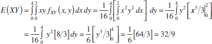
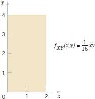
FIGURE 5-15 Random variables with zero covariance from Example 5-22.
Also,
Thus,
![]()
It can be shown that these two random variables are independent. You can check that fXY(x, y) = fX(x)fY(y) for all x and y.
However, if the correlation between two random variables is zero, we cannot immediately conclude that the random variables are independent. Figure 5-12(d) provides an example.
EXERCISES FOR SECTION 5-2
![]() Problem available in WileyPLUS at instructor's discretion.
Problem available in WileyPLUS at instructor's discretion.
![]() Go Tutorial Tutoring problem available in WileyPLUS at instructor's discretion.
Go Tutorial Tutoring problem available in WileyPLUS at instructor's discretion.
5-33. ![]() Determine the covariance and correlation for the following joint probability distribution:
Determine the covariance and correlation for the following joint probability distribution:
5-34. ![]() Determine the covariance and correlation for the following joint probability distribution:
Determine the covariance and correlation for the following joint probability distribution:
![]()
5-35. ![]() Determine the value for c and the covariance and correlation for the joint probability mass function fXY(x, y) = c(x+ y) for x = 1,2,3 and y = 1,2,3.
Determine the value for c and the covariance and correlation for the joint probability mass function fXY(x, y) = c(x+ y) for x = 1,2,3 and y = 1,2,3.
5-36. ![]() Determine the covariance and correlation for the joint proba.bility distribution shown in Fig. 5-10(a) and described in Example 5-10.
Determine the covariance and correlation for the joint proba.bility distribution shown in Fig. 5-10(a) and described in Example 5-10.
5-37. ![]() Patients are given a drug treatment and then evaluated. Symptoms either improve, degrade, or remain the same with probabilities 0.4, 0.1, 0.5, respectively. Assume that four independent patients are treated and let X and Y denote the number of patients who improve or degrade. Are X and Y independent? Calculate the covariance and correlation between X and Y.
Patients are given a drug treatment and then evaluated. Symptoms either improve, degrade, or remain the same with probabilities 0.4, 0.1, 0.5, respectively. Assume that four independent patients are treated and let X and Y denote the number of patients who improve or degrade. Are X and Y independent? Calculate the covariance and correlation between X and Y.
5-38. For the Transaction Processing Performance Council's benchmark in Exercise 5-10, let X, Y, and Z denote the average number of selects, updates, and inserts operations required for each type of transaction, respectively. Calculate the following:
(a) Covariance between X and Y
(b) Correlation between X and Y
(c) Covariance between X and Z
(d) Correlation between X and Z
5-39. ![]() Determine the value for c and the covariance and correlation for the joint probability density function fXY(x, y) = cxy over the range 0 < x < 3 and 0 < y < x.
Determine the value for c and the covariance and correlation for the joint probability density function fXY(x, y) = cxy over the range 0 < x < 3 and 0 < y < x.
5-40. ![]() Determine the value for c and the covariance and correlation for the joint probability density function fXY(x, y) = c over the range 0 < x < 5, 0 < y, and x −1 < y < x +1.
Determine the value for c and the covariance and correlation for the joint probability density function fXY(x, y) = c over the range 0 < x < 5, 0 < y, and x −1 < y < x +1.
5-41. Determine the covariance and correlation for the joint probability density function fXY(x, y) = e−x−y over the range 0 < x and 0 < y.
5-42. ![]() Determine the covariance and correlation for the joint probability density function fXY(x, y) =
Determine the covariance and correlation for the joint probability density function fXY(x, y) = ![]() over the range 0 < x and x<y from Example 5-2.
over the range 0 < x and x<y from Example 5-2.
5-43. The joint probability distribution is
Show that the correlation between X and Y is zero but X and Y are not independent.
5-44. Determine the covariance and correlation for the CD4 counts in a month and the following month in Exercise 5-30.
5-45. Determine the covariance and correlation for the lengths of the minor and major axes in Exercise 5-29.
5-46. Suppose that X and Y are independent continuous random variables. Show that σXY = 0.
5-47. ![]() Suppose that the correlation between X and Y is ρ. For constants a,b,c, and d, what is the correlation between the random variables U = aX + b and V = cY + d?
Suppose that the correlation between X and Y is ρ. For constants a,b,c, and d, what is the correlation between the random variables U = aX + b and V = cY + d?
5-3 Common Joint Distributions
5-3.1 MULTINOMIAL PROBABILITY DISTRIBUTION
The binomial distribution can be generalized to generate a useful joint probability distribution for multiple discrete random variables. The random experiment consists of a series of independent trials. However, the outcome from each trial is categorized into one of k classes. The random variables of interest count the number of outcomes in each class.
Example 5-21 Digital Channel We might be interested in a probability such as the following. Of the 20 bits received, what is the probability that 14 are excellent, 3 are good, 2 are fair, and 1 is poor? Assume that the classifications of individual bits are independent events and that the probabilities of E, G, F, and P are 0.6, 0.3, 0.08, and 0.02, respectively. One sequence of 20 bits that produces the specified numbers of bits in each class can be represented as
![]()
Using independence, we find that the probability of this sequence is
![]()
Clearly, all sequences that consist of the same numbers of E's, G's, F's, and P's have the same probability. Consequently, the requested probability can be found by multiplying 2.708×10⁻⁹ by the number of sequences with 14 E's, 3 G's, 2 F's, and 1P. The number of sequences is found from Chapter 2 to be
![]()
Therefore, the requested probability is
![]()
Example 5-24 leads to the following generalization of a binomial experiment and a binomial distribution.
Suppose that a random experiment consists of a series of n trials. Assume that
(1) The result of each trial is classified into one of k classes.
(2) The probability of a trial generating a result in class 1, class 2, . . ., class k is constant over the trials and equal to p1, p2,..., pk, respectively.
(3) The trials are independent.
The random variables X1, X2,..., Xk that denote the number of trials that result in class 1, class 2, . . ., class k, respectively, have a multinomial distribution and the joint probability mass function is
![]()
for x1 + x2 + . . . + xk = n and p1 + p2 + . . . + pk = 1.
The multinomial distribution is considered a multivariable extension of the binomial distribution.
Example 5-25 Digital Channel In Example 5-24, let the random variables X1, X2, X3, and X4 denote the number of bits that are E, G, F, and P, respectively, in a transmission of 20 bits. The probability that 12 of the bits received are E, 6 are G, 2 are F, and 0 are P is
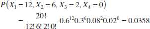
Each trial in a multinomial random experiment can be regarded as either generating or not generating a result in class i, for each i = 1,2,..., k. Because the random variable Xi is the number of trials that result in class i, Xi has a binomial distribution.
Mean and Variance
If X1, X2,..., Xk have a multinomial distribution, the marginal probability distribution of Xi is binomial with
![]()
Example 5-26 Marginal Probability Distributions In Example 5-25, the marginal probability distribution of X2 is binomial with n = 20 and p = 0.3. Furthermore, the joint marginal probability distribution of X2 and X3 is found as follows. The P(X2 = x2, X3 = x3) is the probability that exactly x2 trials result in G and that x3 result in F. The remaining n − x2 − x3 trials must result in either E or P. Consequently, we can consider each trial in the experiment to result in one of three classes: {G}, {F}, and {E, P} with probabilities 0.3, 0.08, and 0.6+0.02 = 0.62, respectively. With these new classes, we can consider the trials to comprise a new multinomial experiment. Therefore,
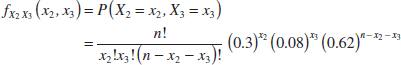
The joint probability distribution of other sets of variables can be found similarly.
5-3.2 BIVARIATE NORMAL DISTRIBUTION
An extension of a normal distribution to two random variables is an important bivariate probability distribution. The joint probability distribution can be defined to handle positive, negative, or zero correlation between the random variables.
Example 5-27 Bivariate Normal Distribution At the start of this chapter, the length of different dimensions of an injection-molded part were presented as an example of two random variables. If the specifications for X and Y are 2.95 to 3.05 and 7.60 to 7.80 millimeters, respectively, we might be interested in the probability that a part satisfies both specifications; that is, P(2.95 < X < 3.05, 7.60 < Y < 7.80). Each length might be modeled by a normal distribution. However, because the measurements are from the same part, the random variables are typically not independent. Therefore, a probability distribution for two normal random varsiables that are not independent is important in many applications.
Bivariate Normal Probability Density Function
The probability density function of a bivariate normal distribution is
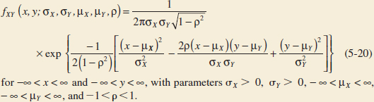
The result that ![]() integrates to 1 is left as an exercise. Also, the bivariate normal probability density function is positive over the entire plane of real numbers.
integrates to 1 is left as an exercise. Also, the bivariate normal probability density function is positive over the entire plane of real numbers.
Two examples of bivariate normal distributions along with corresponding contour plots are illustrated in Fig. 5-16. Each curve on the contour plots is a set of points for which the probability density function is constant. As seen in the contour plots, the bivariate normal probability density function is constant on ellipses in the (x,y) plane. (We can consider a circle to be a special case of an ellipse.) The center of each ellipse is at the point (μX, μY). If ρ > 0(ρ < 0), the major axis of each ellipse has positive (negative) slope, respectively. If ρ = 0, the major axis of the ellipse is aligned with either the x or y coordinate axis.
Example 5-28 The joint probability density function
![]()
is a special case of a bivariate normal distribution with σX = 1, σy = 1, μX = 0, μy = 0, and ρ = 0. This probability density function is illustrated in Fig. 5-17. Notice that the contour plot consists of concentric circles about the origin.
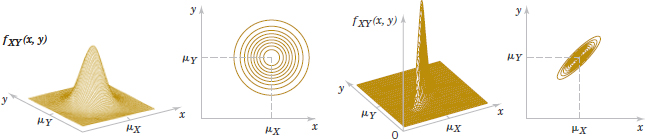
FIGURE 5-16 Examples of bivariate normal distributions.
The following results can be shown for a bivariate normal distribution. The details are left as an exercise.
Marginal Distributions of Bivariate Normal Random Variables
Conditional Distribution of Bivariate Normal Random Variables
If X and Y have a bivariate normal distribution with joint probability density fXY(x,y,σX,σY,μX,μY,ρ), the conditional probability distribution of Y given X = x is normal with mean
![]()
and variance
![]()
Furthermore, as the notation suggests, ρ represents the correlation between X and Y. The following result is left as an exercise.
Correlation of Bivariate Normal Random Variables

The contour plots in Fig. 5-16 illustrate that as ρ moves from 0 (left graph) to 0.9 (right graph), the ellipses narrow around the major axis. The probability is more concentrated about a line in the (x,y) plane and graphically displays greater correlation between the variables. If ρ = −1 or +1, all the probability is concentrated on a line in the (x,y) plane. That is, the probability that X and Y assume a value that is not on the line is zero. In this case, the bivariate normal probability density is not defined.
In general, zero correlation does not imply independence. But in the special case that X and Y have a bivariate normal distribution, if p = 0, X and Y are independent. The details are left as an exercise.
For Bivariate Normal Random Variables Zero Correlation Implies Independence

An important use of the bivariate normal distribution is to calculate probabilities involving two correlated normal random variables.
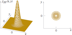
FIGURE 5-17 Bivariate normal probability density function with σx = 1, σy = 1, ρ = 0, μx = 0 μX = 0, and μy = 0.
Example 5-29 Injection-Molded Part Suppose that the X and Y dimensions of an injection-molded part have a bivariate normal distribution with σX = 0.04,σY = 0.08, μX = 3.00, μY = 7.70, and ρ = 0.8. Then the probability that a part satisfies both specifications is
![]()
This probability can be obtained by integrating fXY(x,y;σX,σY,μX,μY,ρ) over the region 2.95 < x<3.05 and 7.60 < y<7.80, as shown in Fig. 5-3. Unfortunately, there is often no closed-form solution to probabilities involving bivariate normal distributions. In this case, the integration must be done numerically.
EXERCISES FOR SECTION 5-3
![]() Problem available in WileyPLUS at instructor's discretion.
Problem available in WileyPLUS at instructor's discretion.
![]() Go Tutorial Tutoring problem available in WileyPLUS at instructor's discretion.
Go Tutorial Tutoring problem available in WileyPLUS at instructor's discretion.
5-48. Test results from an electronic circuit board indicate that 50% of board failures are caused by assembly defects, 30% by electrical components, and 20% by mechanical defects. Suppose that 10 boards fail independently. Let the random variables X, Y, and Z denote the number of assembly, electrical, and mechanical defects among the 10 boards.
Calculate the following:
(a) P(X = 5, Y = 3, Z = 2)
(b) P(X = 8)
(c) P(X = 8|Y = 1)
(d) P(X ≥ 8|Y = 1)
(e) P(X = 7, Y = 1|Z = 2)
5-49. ![]() Based on the number of voids, a ferrite slab is classified as either high, medium, or low. Historically, 5% of the slabs are classified as high, 85% as medium, and 10% as low. A sample of 20 slabs is selected for testing. Let X, Y, and Z denote the number of slabs that are independently classified as high, medium, and low, respectively.
Based on the number of voids, a ferrite slab is classified as either high, medium, or low. Historically, 5% of the slabs are classified as high, 85% as medium, and 10% as low. A sample of 20 slabs is selected for testing. Let X, Y, and Z denote the number of slabs that are independently classified as high, medium, and low, respectively.
(a) What are the name and the values of the parameters of the joint probability distribution of X, Y, and Z?
(b) What is the range of the joint probability distribution of X, Y, and Z?
(c) What are the name and the values of the parameters of the marginal probability distribution of X?
(d) Determine E(X) and V(X).
Determine the following:
(e) P(X = 1, Y = 17, Z = 3)
(f) P(X ≤ 1, Y = 17, Z = 3)
(g) P(X ≤ 1)
(h) E(Y)
(i) P(X = 2, Z = 3|Y = 17)
(j) P(X = 2|Y = 17)
(k) E(X|Y = 17)
5-50. A Web site uses ads to route visitors to one of four landing pages. The probabilities for each landing page are equal. Consider 20 independent visitors and let the random variables W, X, Y, and Z denote the number of visitors routed to each page.
Calculate the following:
(a) P(W = 5, X = 5, Y = 5, Z = 5)
(b) P(W = 5, X = 5, Y = 5, Z = 5)
(c) P(W = 7, X = 7, Y = 6|Z = 3)
(d) P(W = 7, X = 7, Y = 3|Z = 3)
(e) P(W ≤ 2)
(f) E(W)
(g) P(W = 5, X = 5)
(h) P(W = 5|X = 5)
5-51. Four electronic ovens that were dropped during shipment are inspected and classified as containing either a major, a minor, or no defect. In the past, 60% of dropped ovens had a major defect, 30% had a minor defect, and 10% had no defect. Assume that the defects on the four ovens occur independently.
(a) ![]() Is the probability distribution of the count of ovens in each category multinomial? Why or why not?
Is the probability distribution of the count of ovens in each category multinomial? Why or why not?
(b) ![]() What is the probability that, of the four dropped ovens, two have a major defect and two have a minor defect?
What is the probability that, of the four dropped ovens, two have a major defect and two have a minor defect?
(c) What is the probability that no oven has a defect?
Determine the following:
(d) Joint probability mass function of the number of ovens with a major defect and the number with a minor defect
(e) Expected number of ovens with a major defect
(f) Expected number of ovens with a minor defect
(g) Conditional probability that two ovens have major defects given that two ovens have minor defects
(h) Conditional probability that three ovens have major defects given that two ovens have minor defects
(i) Conditional probability distribution of the number of ovens with major defects given that two ovens have minor defects
(j) Conditional mean of the number of ovens with major defects given that two ovens have minor defects.
5-52. Let X and Y represent the concentration and viscosity of a chemical product. Suppose that X and Y have a bivariate normal distribution with σX = 4, σY = 1, μX = 2 and μy = 1. Draw a rough contour plot of the joint probability density function for each of the following values of ρ:
(a) ρ = 0
(b) ρ = 0.8
(c) ρ = −0.8
5-53. ![]() Suppose that X and Y have a bivariate normal distribution with σX = 0.04, σY = 0.08, μX = 3.00, μY = 7.70, and ρ = 0.
Suppose that X and Y have a bivariate normal distribution with σX = 0.04, σY = 0.08, μX = 3.00, μY = 7.70, and ρ = 0.
Determine the following:
(a) P(2.95 < X < 3.05)
(b) P(7.60 < Y < 7.80)
(c) P(2.95 < X < 3.05, 7.60 < Y < 7.80)
5-54. ![]() In an acid-base titration, a base or acid is gradually added to the other until they have completely neutralized each other. Let X and Y denote the milliliters of acid and base needed for equivalence, respectively. Assume that X and Y have a bivariate normal distribution with σX = 5 mL, σY = 2 mL, μX = 120 mL, μY = 100 mL, and ρ = 0.6.
In an acid-base titration, a base or acid is gradually added to the other until they have completely neutralized each other. Let X and Y denote the milliliters of acid and base needed for equivalence, respectively. Assume that X and Y have a bivariate normal distribution with σX = 5 mL, σY = 2 mL, μX = 120 mL, μY = 100 mL, and ρ = 0.6.
(a) Covariance between X and Y
(b) Marginal probability distribution of X
(c) P(X < 116)
(d) Conditional probability distribution of X given that Y = 102
(e) P(X < 116|Y = 102)
5-55. ![]() In the manufacture of electroluminescent lamps, several different layers of ink are deposited onto a plastic substrate. The thickness of these layers is critical if specifications regarding the final color and intensity of light are to be met. Let X and Y denote the thickness of two different layers of ink. It is known that X is normally distributed with a mean of 0.1 millimeter and a standard deviation of 0.00031 millimeter, and Y is normally distributed with a mean of 0.23 millimeter and a standard deviation of 0.00017 millimeter. The value of ρ for these variables is equal to 0. Specifications call for a lamp to have a thickness of the ink corresponding to X in the range of 0.099535 to 0.100465 millimeter and Y in the range of 0.22966 to 0.23034 millimeter. What is the probability that a randomly selected lamp will conform to specifications?
In the manufacture of electroluminescent lamps, several different layers of ink are deposited onto a plastic substrate. The thickness of these layers is critical if specifications regarding the final color and intensity of light are to be met. Let X and Y denote the thickness of two different layers of ink. It is known that X is normally distributed with a mean of 0.1 millimeter and a standard deviation of 0.00031 millimeter, and Y is normally distributed with a mean of 0.23 millimeter and a standard deviation of 0.00017 millimeter. The value of ρ for these variables is equal to 0. Specifications call for a lamp to have a thickness of the ink corresponding to X in the range of 0.099535 to 0.100465 millimeter and Y in the range of 0.22966 to 0.23034 millimeter. What is the probability that a randomly selected lamp will conform to specifications?
5-56. Patients given drug therapy either improve, remain the same, or degrade with probabilities 0.5, 0.4, 0.1, respectively. Suppose that 20 patients (assumed to be independent) are given the therapy. Let X1, X2, and X3 denote the number of patients who improved, stayed the same, or became degraded. Determine the following.
(a) Are X1, X2, X3 independent?
(b) P(X1 = 10)
(c) P(X1 = 10,X2 = 8,X3 = 2)
(d) P(X1 = 5|X2 = 12)
(e) E(X1)
5-57. Suppose that X has a standard normal distribution. Let the conditional distribution of Y given X = x be normally distributed with mean E(Y|x) = 2x and variance V(Y|x) = 2x. Determine the following.
(a) Are X and Y independent?
(b) P(Y < 3|X = 3)
(c) E(Y|X = 3)
(d) fXY(x,y)
(e) Recognize the distribution fXY(x, y) and identify the mean and variance of Y and the correlation between X and Y.
5-58. Suppose that X and Y have a bivariate normal distribution with joint probability density function fXY(x,y;σX,σY,μX,μY,ρ)
(a) Show that the conditional distribution of Y given that X = x is normal.
(b) ![]() Determine E(Y|X = x).
Determine E(Y|X = x).
(c) ![]() Determine V(Y|X = x).
Determine V(Y|X = x).
5-59. If X and Y have a bivariate normal distribution with ρ = 0, show that X and Y are independent.
5-60. Show that the probability density function fXY(x,y;σX,σY,μX,μY,ρ) of a bivariate normal distribution integrates to 1. [Hint: Complete the square in the exponent and use the fact that the integral of a normal probability density function for a single variable is 1.]
5-61. If X and Y have a bivariate normal distribution with joint probability density fXY(x,y;σX,σY,μX,μY,ρ), show that the marginal probability distribution of X is normal with mean μx and standard deviation σx. [Hint: Complete the square in the exponent and use the fact that the integral of a normal probability density function for a single variable is 1.]
5-4 Linear Functions of Random Variables
A random variable is sometimes defined as a function of one or more random variables. In this section, results for linear functions are highlighted because of their importance in the remainder of the book. For example, if the random variables X1 and X2 denote the length and width, respectively, of a manufactured part, Y = 2X1 + 2X2 is a random variable that represents the perimeter of the part. As another example, recall that the negative binomial random variable was represented as the sum of several geometric random variables.
In this section, we develop results for random variables that are linear combinations of random variables.
Linear Combination
Given random variables X1, X2,..., Xp and constants c1, c2,. . .cp,
![]()
is a linear combination of X1, X2,..., Xp.
Now E(Y) can be found from the joint probability distribution of X1, X2,..., Xp as follows. Assume that X1, X2, Xp are continuous random variables. An analogous calculation can be used for discrete random variables.
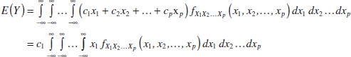
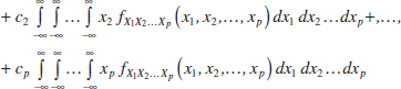
By using Equation 5-10 for each of the terms in this expression, we obtain the following.
Mean of a Linear Function
If Y = c1X1 + c2X2 + . . . + cpXp,
![]()
Furthermore, it is left as an exercise to show the following.
Variance of a Linear Function
If X1, X2,..., Xp are random variables, and Y = c1X1 + c2X2 + . . . + cpXp, then in general,
![]()
If X1, X2,..., Xp are independent,
![]()
Note that the result for the variance in Equation 5-27 requires the random variables to be independent. To see why the independence is important, consider the following simple example. Let X1 denote any random variable and define X2 = −X1. Clearly, X1 and X2 are not independent. In fact, ρXY = −1. Now Y = X1 + X2 is 0 with probability 1. Therefore, V(Y) = 0 regardless of the variances of X1 and X2.
Example 5-30 Negative Binomial Distribution In Chapter 3, we found that if Y is a negative binomial random variable with parameters p and r, Y = X1 + X2 + . . . + Xr, where each Xi is a geometric random variable with parameter p, and they are independent. Therefore, E(Xi) = 1/p and V(Xi) = (1 − p)/p2. From Equation 5-25, E(Y) = r/p, and from Equation 5-27, V(Y) = r(1 − p)/p2.
An approach similar to the one applied in Example 5-30 can be used to verify the formulas for the mean and variance of an Erlang random variable in Chapter 4. An important use of Equation 5-27 is in error propagation, which is presented in the following example.
Example 5-31 Error Propagation A semiconductor product consists of three layers. Supposing that the variances in thickness of the first, second, and third layers are 25, 40, and 30 square nanometers, respectively, and the layer thicknesses are independent. What is the variance of the thickness of the final product?
Let X1, X2, X3, and X be random variables that denote the thicknesses of the respective layers, and the final product. Then,
![]()
The variance of X is obtained from Equation 5-27:
![]()
Consequently, the standard deviation of thickness of the final product is 951/2 = 9.75 nm, and this shows how the variation in each layer is propagated to the final product.
The particular linear function that represents the average of random variables with identical means and variances is used quite often in subsequent chapters. We highlight the results for this special case.
Mean and Variance of an Average
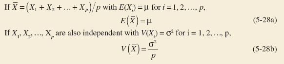
The conclusion for V(![]() ) is obtained as follows. Using Equation 5-27 with ci = 1/p and V(Xi) = σ2 yields
) is obtained as follows. Using Equation 5-27 with ci = 1/p and V(Xi) = σ2 yields
![]()
Another useful result concerning linear functions of random variables is a reproductive property that holds for independent, normal random variables.
Reproductive Property of the Normal Distribution
If X1, X2, . . ., Xp are independent, normal random variables with E(Xi) = μi and V(Xi) = ![]() , for i = 1, 2,. . .p,
, for i = 1, 2,. . .p,
![]()
is a normal random variable with
![]()
and
![]()
The mean and variance of Y follow from Equations 5-25 and 5-27. The fact that Y has a normal distribution can be obtained from moment generating functions in a later section of this chapter.
Example 5-32 Linear Function of Independent Normal Random Variables Let the random variables X1 and X2 denote the length and width, respectively, of a manufactured part. Assume that X1 is normal with E(X1) = 2 cm and standard deviation 0.1 cm and that X2 is normal with E(X2) = 5 cm and standard deviation 0.2 cm. Also assume that X1 and X2 are independent. Determine the probability that the perimeter exceeds 14.5 cm.
Then Y = 2X1 + 2X2 is a normal random variable that represents the perimeter of the part. We obtain E(Y) = 14 cm and the variance of Y is
![]()
Now
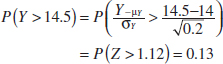
Example 5-33 Beverage Volume An automated filling machine fills soft-drink cans. The mean fill volume is 12.1 fluid ounces, and the standard deviation is 0.1 oz. Assume that the fill volumes of the cans are independent, normal random variables. What is the probability that the average volume of 10 cans selected from this process is less than 12 oz?
Let X1, X2,..., X10 denote the fill volumes of the 10 cans. The average fill volume (denoted as ![]() ) is a normal random variable with
) is a normal random variable with
![]()
Consequently,
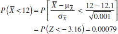
EXERCISES FOR SECTION 5-4
![]() Problem available in WileyPLUS at instructor's discretion.
Problem available in WileyPLUS at instructor's discretion.
![]() Go Tutorial Tutoring problem available in WileyPLUS at instructor's discretion.
Go Tutorial Tutoring problem available in WileyPLUS at instructor's discretion.
5-62. ![]() X and Y are independent, normal random variables with E(X) = 0, V(X) = 4, E(Y) = 10, and V(Y) = 9.
X and Y are independent, normal random variables with E(X) = 0, V(X) = 4, E(Y) = 10, and V(Y) = 9.
Determine the following:
(a) E(2X + 3Y)
(b) V(2X + 3Y)
(c) P(2X + 3Y < 30)
(d) P(2X + 3Y < 40)
5-63. X and Y are independent, normal random variables with E(X) = 2, V(X) = 5, E(Y) = 6, and V(Y) = 8.
Determine the following:
(a) E(3X + 2Y)
(b) V(3X + 2Y)
(c) P(3X + 2Y < 18)
(d) P(3X + 2Y < 28)
5-64. ![]() Suppose that the random variable X represents the length of a punched part in centimeters. Let Y be the length of the part in millimeters. If E(X) = 5 and V(X) = 0.25, what are the mean and variance of Y?
Suppose that the random variable X represents the length of a punched part in centimeters. Let Y be the length of the part in millimeters. If E(X) = 5 and V(X) = 0.25, what are the mean and variance of Y?
5-65. ![]() A plastic casing for a magnetic disk is composed of two halves. The thickness of each half is normally distributed with a mean of 2 millimeters, and a standard deviation of 0.1 millimeter and the halves are independent.
A plastic casing for a magnetic disk is composed of two halves. The thickness of each half is normally distributed with a mean of 2 millimeters, and a standard deviation of 0.1 millimeter and the halves are independent.
(a) Determine the mean and standard deviation of the total thickness of the two halves.
(b) What is the probability that the total thickness exceeds 4.3 millimeters?
5-66. ![]() Making handcrafted pottery generally takes two major steps: wheel throwing and firing. The time of wheel throwing and the time of firing are normally distributed random variables with means of 40 minutes and 60 minutes and standard deviations of 2 minutes and 3 minutes, respectively.
Making handcrafted pottery generally takes two major steps: wheel throwing and firing. The time of wheel throwing and the time of firing are normally distributed random variables with means of 40 minutes and 60 minutes and standard deviations of 2 minutes and 3 minutes, respectively.
(a) What is the probability that a piece of pottery will be finished within 95 minutes?
(b) What is the probability that it will take longer than 110 minutes?
5-67. ![]() In the manufacture of electroluminescent lamps, several different layers of ink are deposited onto a plastic substrate. The thickness of these layers is critical if specifications regarding the final color and intensity of light are to be met. Let X and Y denote the thickness of two different layers of ink. It is known that X is normally distributed with a mean of 0.1 mm and a standard deviation of 0.00031 mm, and Y is also normally distributed with a mean of 0.23 mm and a standard deviation of 0.00017 mm. Assume that these variables are independent.
In the manufacture of electroluminescent lamps, several different layers of ink are deposited onto a plastic substrate. The thickness of these layers is critical if specifications regarding the final color and intensity of light are to be met. Let X and Y denote the thickness of two different layers of ink. It is known that X is normally distributed with a mean of 0.1 mm and a standard deviation of 0.00031 mm, and Y is also normally distributed with a mean of 0.23 mm and a standard deviation of 0.00017 mm. Assume that these variables are independent.
(a) If a particular lamp is made up of these two inks only, what is the probability that the total ink thickness is less than 0.2337 mm?
(b) A lamp with a total ink thickness exceeding 0.2405 mm lacks the uniformity of color that the customer demands. Find the probability that a randomly selected lamp fails to meet customer specifications.
5-68. ![]() The width of a casing for a door is normally distributed with a mean of 24 inches and a standard deviation of 1/8 inch. The width of a door is normally distributed with a mean of 23 7/8 inches and a standard deviation of 1/16 inch. Assume independence.
The width of a casing for a door is normally distributed with a mean of 24 inches and a standard deviation of 1/8 inch. The width of a door is normally distributed with a mean of 23 7/8 inches and a standard deviation of 1/16 inch. Assume independence.
(a) Determine the mean and standard deviation of the difference between the width of the casing and the width of the door.
(b) What is the probability that the width of the casing minus the width of the door exceeds 1/4 inch?
(c) What is the probability that the door does not fit in the casing?
5-69. ![]() An article in Knee Surgery Sports Traumatology, Arthroscopy [“Effect of Provider Volume on Resource Utilization for Surgical Procedures” (2005, Vol. 13, pp. 273–279)] showed a mean time of 129 minutes and a standard deviation of 14 minutes for ACL reconstruction surgery for high-volume hospitals (with more than 300 such surgeries per year). If a high-volume hospital needs to schedule 10 surgeries, what are the mean and variance of the total time to complete these surgeries? Assume that the times of the surgeries are independent and normally distributed.
An article in Knee Surgery Sports Traumatology, Arthroscopy [“Effect of Provider Volume on Resource Utilization for Surgical Procedures” (2005, Vol. 13, pp. 273–279)] showed a mean time of 129 minutes and a standard deviation of 14 minutes for ACL reconstruction surgery for high-volume hospitals (with more than 300 such surgeries per year). If a high-volume hospital needs to schedule 10 surgeries, what are the mean and variance of the total time to complete these surgeries? Assume that the times of the surgeries are independent and normally distributed.
5-70. ![]() An automated filling machine fills soft-drink cans, and the standard deviation is 0.5 fluid ounce. Assume that the fill volumes of the cans are independent, normal random variables.
An automated filling machine fills soft-drink cans, and the standard deviation is 0.5 fluid ounce. Assume that the fill volumes of the cans are independent, normal random variables.
(a) What is the standard deviation of the average fill volume of 100 cans?
(b) If the mean fill volume is 12.1 oz, what is the probability that the average fill volume of the 100 cans is less than 12 oz?
(c) What should the mean fill volume equal so that the probability that the average of 100 cans is less than 12 oz is 0.005?
(d) If the mean fill volume is 12.1 oz, what should the standard deviation of fill volume equal so that the probability that the average of 100 cans is less than 12 oz is 0.005?
(e) Determine the number of cans that need to be measured such that the probability that the average fill volume is less than 12 oz is 0.01.
5-71. ![]() The photoresist thickness in semiconductor manufacturing has a mean of 10 micrometers and a standard deviation of 1 micrometer. Assume that the thickness is normally distributed and that the thicknesses of different wafers are independent.
The photoresist thickness in semiconductor manufacturing has a mean of 10 micrometers and a standard deviation of 1 micrometer. Assume that the thickness is normally distributed and that the thicknesses of different wafers are independent.
(a) Determine the probability that the average thickness of 10 wafers is either more than 11 or less than 9 micrometers.
(b) Determine the number of wafers that need to be measured such that the probability that the average thickness exceeds 11 micrometers is 0.01.
(c) If the mean thickness is 10 micrometers, what should the standard deviation of thickness equal so that the probability that the average of 10 wafers is either more than 11 or less than 9 micrometers is 0.001?
5-72. ![]() Assume that the weights of individuals are independent and normally distributed with a mean of 160 pounds and a standard deviation of 30 pounds. Suppose that 25 people squeeze into an elevator that is designed to hold 4300 pounds.
Assume that the weights of individuals are independent and normally distributed with a mean of 160 pounds and a standard deviation of 30 pounds. Suppose that 25 people squeeze into an elevator that is designed to hold 4300 pounds.
(a) What is the probability that the load (total weight) exceeds the design limit?
(b) What design limit is exceeded by 25 occupants with probability 0.0001?
5-73. Weights of parts are normally distributed with variance σ2. Measurement error is normally distributed with mean 0 and variance 0.5σ2, independent of the part weights, and adds to the part weight. Upper and lower specifications are centered at 3σ about the process mean.
(a) Without measurement error, what is the probability that a part exceeds the specifications?
(b) With measurement error, what is the probability that a part is measured as being beyond specifications? Does this imply it is truly beyond specifications?
(c) What is the probability that a part is measured as being beyond specifications if the true weight of the part is 1 σ below the upper specification limit?
5-74. A U-shaped component is to be formed from the three parts A, B, and C. See Fig. 5-18. The length of A is normally distributed with a mean of 10 mm and a standard deviation of 0.1 mm. The thickness of parts B and C is normally distributed with a mean of 2 mm and a standard deviation of 0.05 mm. Assume that all dimensions are independent.
(a) Determine the mean and standard deviation of the length of the gap D.
(b) What is the probability that the gap D is less than 5.9 mm?
5-75. Consider the perimeter of a part in Example 5-32. Let X1 and X2 denote the length and width of a part with standard deviations 0.1 and 0.2 centimeters, respectively. Suppose that the covariance between X1 and X2 is 0.02. Determine the variance of the perimeter Y = 2X1 + 2X2 of a part. Compare and comment on the result here and in the example.
5-76. Three electron emitters produce electron beams with changing kinetic energies that are uniformly distributed in the ranges [3, 7], [2, 5], and [4, 10]. Let Y denote the total kinetic energy produced by these electron emitters.
(a) Suppose that the three beam energies are independent. Determine the mean and variance of Y.
(b) Suppose that the covariance between any two beam energies is −0.5. Determine the mean and variance of Y.
(c) Compare and comment on the results in parts (a) and (b).
5-77. In Exercise 5-31, the monthly demand for MMR vaccine was assumed to be approximately normally distributed with a mean and standard deviation of 1.1 and 0.3 million doses, respectively. Suppose that the demands for different months are independent, and let Z denote the demand for a year (in millions of does). Determine the following:
(a) Mean, variance, and distribution of Z
(b) P(Z<13.2)
(c) P(11<Z<15)
(d) Value for c such that P(Z<c) = 0.99
5-78. The rate of return of an asset is the change in price divided by the initial price (denoted as r). Suppose that $10,000 is used to purchase shares in three stocks with rates of returns X1, X2, X3. Initially, $2500, $3000, and $4500 are allocated to each one, respectively. After one year, the distribution of the rate of return for each is normally distributed with the following parameters: μ1 = 0.12,σ1 = 0.14,μ2 = 0.04,σ2 = 0.02,μ3 = 0.07,σ3 = 0.08.
(a) Assume that these rates of return are independent. Determine the mean and variance of the rate of return after one year for the entire investment of $10,000.
(b) Assume that X1 is independent of X2 and X3 but that the covariance between X2 and X3 is −0.005. Repeat part (a).
(c) Compare the means and variances obtained in parts (a) and (b) and comment on any benefits from negative covariances between the assets.
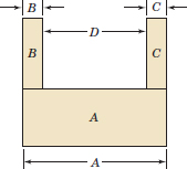
5-5 General Functions of Random Variables
In many situations in statistics, it is necessary to derive the probability distribution of a function of one or more random variables. In this section, we present some results that are helpful in solving this problem.
Suppose that X is a discrete random variable with probability distribution fX(x). Let Y = h(X) be a function of X that defines a one-to-one transformation between the values of X and Y and that we wish to find the probability distribution of Y. By a one-to-one transformation, we mean that each value x is related to one and only one value of y = h(x) and that each value of y is related to one and only one value of x, say, x = u(y) where u(y) is found by solving y = h(x) for x in terms of y.
Now the random variable Y takes on the value y when X takes on the value u(y). Therefore, the probability distribution of Y is
![]()
We may state this result as follows.
General Function of a Discrete Random Variable
Suppose that X is a discrete random variable with probability distribution fX(x). Let Y = h(X) define a one-to-one transformation between the values of X and Y so that the equation y = h(x) can be solved uniquely for x in terms of y. Let this solution be x = u(y). Then the probability mass function of the random variable Y is
![]()
Example 5-34 Function of a Discrete Random Variable Let X be a geometric random variable with probability distribution
![]()
Find the probability distribution of Y = X2.
Because X ≥ 0, the transformation is one to one; that is, y = x2 and x = ![]() . Therefore, Equation 5-30 indicates that the distribution of the random variable Y is
. Therefore, Equation 5-30 indicates that the distribution of the random variable Y is
![]()
We now consider the situation in which the random variables are continuous. Let Y = h(X) with X continuous and the transformation one to one.
General Function of a Continuous Random Variable
Suppose that X is a continuous random variable with probability distribution fX(x). The function Y = h(X) is a one-to-one transformation between the values of Y and X, so that the equation y = h(x) can be uniquely solved for x in terms of y. Let this solution be x = u(y). The probability distribution of Y is
![]()
where J = u′(y) is called the Jacobian of the transformation and the absolute value of J is used.
Equation 5-31 is shown as follows. Let the function y = h(x) be an increasing function of x. Now
![]()
If we change the variable of integration from x to y by using x = u(y), we obtain dx = u′(y)dy and then
![]()
Because the integral gives the probability that Y ≤ a for all values of a contained in the feasible set of values for y, fX[u(y)]u′(y) must be the probability density of Y. Therefore, the probability distribution of Y is
![]()
If the function y = h(x) is a decreasing function of x, a similar argument holds.
Example 5-35 Function of a Continuous Random Variable Let X be a continuous random variable with probability distribution
![]()
Find the probability distribution of Y = h(X) = 2X + 4.
Note that y = h(x) = 2x + 4 is an increasing function of x. The inverse solution is x = u(y) = (y − 4)/2, and from this, we find the Jacobian to be J = u′(y) = dx/dy = 1/2. Therefore, from Equation 5-31, the probability distribution of Y is
![]()
EXERCISES FOR SECTION 5-5
![]() Problem available in WileyPLUS at instructor's discretion.
Problem available in WileyPLUS at instructor's discretion.
![]() Go Tutorial Tutoring problem available in WileyPLUS at instructor's discretion
Go Tutorial Tutoring problem available in WileyPLUS at instructor's discretion
5-79. ![]() Suppose that X is a random variable with probability distribution
Suppose that X is a random variable with probability distribution
fX(x) = 1/4, x = 1,2,3,4
Determine the probability distribution of Y = 2X + 1.
5-80. Let X be a binomial random variable with p = 0.25 and n = 3. Determine the probability distribution of the random variable Y = X2.
5-81. ![]() Suppose that X is a continuous random variable with probability distribution
Suppose that X is a continuous random variable with probability distribution
![]()
(a) Determine the probability distribution of the random variable Y = 2X + 10.
(b) Determine the expected value of Y.
5-82. Suppose that X has a uniform probability distribution
fX(x) = 1, 0 ≤ x ≤ 1
Show that the probability distribution of the random variable Y = −2X is chi-squared with two degrees of freedom.
5-83. ![]() A random variable X has the probability distribution
A random variable X has the probability distribution
fX(x) = e−x, x≥0
Determine the probability distribution for the following:
(a) Y = X2
(b) Y = X1/2
(c) Y = ln X
5-84. ![]() The velocity of a particle in a gas is a random variable V with probability distribution
The velocity of a particle in a gas is a random variable V with probability distribution
fV(v) = av2e− bv v>0
where b is a constant that depends on the temperature of the gas and the mass of the particle.
(a) Determine the value of the constant a.
(b) The kinetic energy of the particle is W = mV2/2. Determine the probability distribution of W.
5-85. ![]() Suppose that X has the probability distribution
Suppose that X has the probability distribution
fX(x) = 1, 1 ≤ x ≤ 2
Determine the probability distribution of the random variable Y = eX.
5-86. ![]() The random variable X has the probability distribution
The random variable X has the probability distribution
![]()
Determine the probability distribution of Y = (X − 2)2.
5-87. An aircraft is flying at a constant altitude with velocity magnitude r1 (relative to the air) and angle θ1 (in a two-dimensional coordinate system). The magnitude and direction of the wind are r2 and θ2, respectively. Suppose that the wind angle is uniformly distributed between 10 and 20 degrees and all other parameters are constant. Determine the probability density function of the magnitude of the resultant vector r = [![]() + r1r2(cosθ1 − cosθ2)]0.5.
+ r1r2(cosθ1 − cosθ2)]0.5.
5-88. Derive the probability density function for a lognormal random variable Y from the relationship that Y = exp(W) for a normal random variable W with mean θ and variance ω2.
5-89. The computational time of a statistical analysis applied to a data set can sometimes increase with the square of N, the number of rows of data. Suppose that for a particular algorithm, the computation time is approximately T = 0.004N2 seconds. Although the number of rows is a discrete measurement, assume that the distribution of N over a number of data sets can be approximated with an exponential distribution with a mean of 10,000 rows. Determine the probability density function and the mean of T.
5-90. Power meters enable cyclists to obtain power measurements nearly continuously. The meters also calculate the average power generated over a time interval. Professional riders can generate 6.6 watts per kilogram of body weight for extended periods of time. Some meters calculate a normalized power measurement to adjust for the physiological effort required when the power output changes frequently. Let the random variable X denote the power output at a measurement time and assume that X has a lognormal distribution with parameters θ = 5.2933 and ω2 = 0.00995. The normalized power is computed as the fourth root of the mean of Y = X4.
Determine the following:
(a) Mean and standard deviation of X
(b) fY(y)
(c) Mean and variance of Y
(d) Fourth root of the mean of Y
(e) Compare [E(X4)]1/4 to E(X) and comment.
5-6 Moment-Generating Functions
Suppose that X is a random variable with mean μ. Throughout this book we have used the idea of the expected value of the random variable X, and in fact E(X) = μ. Now suppose that we are interested in the expected value of a function of X, g(X) = Xr. The expected value of this function, or E[g(X)] = E(Xr), is called the rth moment about the origin of the random variable X, which we will denote by μ′r.
Definition of Moments about the Origin
The rth moment about the origin of the random variable X is
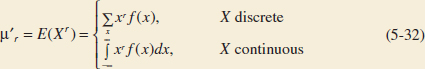
Notice that the first moment about the origin is just the mean, that is, E(X) = μ′1 = μ. Furthermore, since the second moment about the origin is E(X)2 = μ′2, we can write the variance of a random variable in terms of origin moments as follows:
![]()
The moments of a random variable can often be determined directly from the definition in Equation 5-32, but there is an alternative procedure that is frequently useful that makes use of a special function.
Definition of a Moment-Generating Function
The moment-generating function of the random variable X is the expected value of etX and is denoted by MX(t). That is,
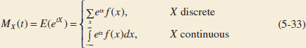
The moment-generating function MX(t) will exist only if the sum or integral in the above definition converges. If the moment-generating function of a random variable does exist, it can be used to obtain all the origin moments of the random variable.
Let X be a random variable with moment-generating function MX(t). Then
![]()
Assuming that we can differentiate inside the summation and integral signs,
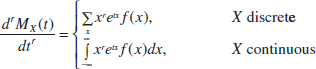
Now if we set t = 0 in this expression, we find that
![]()
Example 5-36 Moment-Generating Function for a Binomial Random Variable Suppose that X has a binomial distribution, that is
![]()
Determine the moment-generating function and use it to verify that the mean and variance of the binomial random variable are μ = np and σ2 = np(1 − p).
From the definition of a moment-generatingfunction, we have
![]()
This last summation is the binomial expansion of [pet + (1 − p)]n, so
![]()
Taking the first and second derivatives, we obtain
![]()
and
![]()
If we set t = 0 in M′X(t), we obtain
![]()
which is the mean of the binomial random variable X. Now if we set t = 0 in ![]() (t),
(t),
![]()
Therefore, the variance of the binomial random variable is
![]()
Example 5-37 Moment-Generating Function for a Normal Random Variable Find the moment-generating function of the normal random variable and use it to show that the mean and variance of this random variable are μ and σ2, respectively.
The moment-generating function is
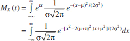
If we complete the square in the exponent, we have
![]()
and then
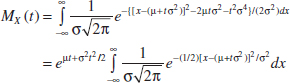
Let u = [x − (μ + tσ2)]/σ. Then dx = σdu, and the last expression above becomes
![]()
Now the integral is just the total area under a standard normal density, which is 1, so the moment-generating function of a normal random variable is
![]()
Differentiating this function twice with respect to t and setting t = 0 in the result, yields
![]()
Therefore, the variance of the normal random variable is
![]()
Moment generating functions have many important and useful properties. One of the most important of these is the uniqueness property. That is, the moment-generating function of a random variable is unique when it exists, so if we have two random variables X and Y, say, with moment-generating functions MX(t) and MY(t), then if MX(t) = MY(t) for all values of t, both X and Y have the same probability distribution. Some of the other useful properties of the moment-generating function are summarized as follows.
Properties of Moment Generating Functions
If X is a random variable and a is a constant, then
![]()
If X1, X2,..., Xn are independent random variables with moment generating functions MX1(t), MX2(t),..., MXn(t), respectively, and if Y = X1 + X2 + ··· + Xn, then the moment generating function of Y is
![]()
Property (1) follows from MX+a(t) = E[et(X + a)] = eat E(etX) = eatMX(t). Property (2) follows from MaX(t) = E[et (aX)] = E[e(at)X] = MX(at). Consider property (3) for the case where the X's are continuous random variables:

Because the X's are independent,
![]()
and one may write
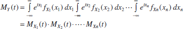
For the case when the X's are discrete, we would use the same approach replacing integrals with summations.
Equation 5-35 is particularly useful. In many situations we need to find the distribution of the sum of two or more independent random variables, and often this result makes the problem very easy. This is illustrated in the following example.
Example 5-38 Distribution of a Sum of Poisson Random Variables Suppose that X1 and X2 are two independent Poisson random variables with parameters λ1 and λ2, respectively. Determine the probability distribution of Y = X1 + X2.
The moment-generating function of a Poisson random variable with parameter λ is
![]()
so the moment-generating functions of X1 and X2 are MX1(t) = eλ1(et −1) and MX2(t) = eλ2(et − 1), respectively. Using Equation 5-35, the moment-generating function of Y = X1 + X2 is
![]()
which is recognized as the moment-generating function of a Poisson random variable with parameter λ1 + λ2. Therefore, the sum of two independent Poisson random variables with parameters λ1 and λ2 is a Poisson random variable with parameter equal to the sum λ1 + λ2.
EXERCISES FOR SECTION 5-6
![]() Problem available in WileyPLUS at instructor's discretion.
Problem available in WileyPLUS at instructor's discretion.
![]() Go Tutorial Tutoring problem available in WileyPLUS at instructor's discretion
Go Tutorial Tutoring problem available in WileyPLUS at instructor's discretion
5-91. A random variable X has the discrete uniform distribution
![]()
(a) Show that the moment-generating function is
![]()
(b) Use MX(t) to find the mean and variance of X.
5-92. A random variable X has the Poisson distribution
![]()
(a) Show that the moment-generating function is
![]()
(b) Use MX(t) to find the mean and variance of the Poisson random variable.
5-93. The geometric random variable X has probability distribution
f(x) = (1 − p)x − 1p, x = 1,2,. . .
Show that the moment-generating function is
![]()
Use MX(t) to find the mean and variance of X.
5-94. The chi-squared random variable with k degrees of freedom has moment-generating function MX(t) = (1 − 2t) − k/2. Suppose that X1 and X2 are independent chi-squared random variables with k1 and k2 degrees of freedom, respectively. What is the distribution of Y = X1 + X2?
5-95. A continuous random variable X has the following probability distribution:
![]()
(a) Find the moment-generating function for X.
(b) Find the mean and variance of X.
5-96. The continuous uniform random variable X has density function
![]()
(a) Show that the moment-generating function is
![]()
(b) Use MX(t) to find the mean and variance of X.
5-97. A random variable X has the exponential distribution
![]()
Show that the moment-generating function of X is
![]()
(b) Find the mean and variance of X.
5-98. A random variable X has the gamma distribution
![]()
(a) Show that the moment-generating function of X is
![]()
(b) Find the mean and variance of X.
5-99. Let X1, X2,..., Xr be independent exponential random variables with parameter λ.
(a) Find the moment-generating function of Y = X1 + X2 + . . . + Xr.
(b) What is the distribution of the random variable Y?
5-100. Suppose that Xi has a normal distribution with mean μi and variance ![]() , i = 1, 2. Let X1 and X2 be independent.
, i = 1, 2. Let X1 and X2 be independent.
(a) Find the moment-generating function of Y = X1 + X1.
(b) What is the distribution of the random variable Y?
Supplemental Exercises
5-101. ![]() Show that the following function satisfies the properties of a joint probability mass function:
Show that the following function satisfies the properties of a joint probability mass function:
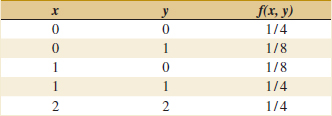
Determine the following:
(a) P(X < 0.5, Y < 1.5)
(b) P(X ≤ 1)
(c) P(X < 1.5)
(d) P(X > 0.5, Y < 1.5)
(e) E(X), E(Y), V(X), V(Y).
(f) Marginal probability distribution of the random variable X
(g) Conditional probability distribution of Y given that X = 1
(h) E(Y|X = 1)
(i) Are X and Y independent? Why or why not?
(j) Correlation between X and Y.
5-102. ![]() The percentage of people given an antirheumatoid medication who suffer severe, moderate, or minor side effects are 10, 20, and 70%, respectively. Assume that people react independently and that 20 people are given the medication.
The percentage of people given an antirheumatoid medication who suffer severe, moderate, or minor side effects are 10, 20, and 70%, respectively. Assume that people react independently and that 20 people are given the medication.
Determine the following:
(a) Probability that 2, 4, and 14 people will suffer severe, moderate, or minor side effects, respectively
(b) Probability that no one will suffer severe side effects
(c) Mean and variance of the number of people who will suffer severe side effects
(d) Conditional probability distribution of the number of people who suffer severe side effects given that 19 suffer minor side effects
(e) Conditional mean of the number of people who suffer severe side effects given that 19 suffer minor side effects
5-103. The backoff torque required to remove bolts in a steel plate is rated as high, moderate, or low. Historically, the probability of a high, moderate, or low rating is 0.6, 0.3, or 0.1, respectively. Suppose that 20 bolts are evaluated and that the torque ratings are independent.
(a) What is the probability that 12, 6, and 2 bolts are rated as high, moderate, and low, respectively?
(b) What is the marginal distribution of the number of bolts rated low?
(c) What is the expected number of bolts rated low?
(d) What is the probability that the number of bolts rated low is more than two?
(e) What is the conditional distribution of the number of bolts rated low given that 16 bolts are rated high?
(f) What is the conditional expected number of bolts rated low given that 16 bolts are rated high?
(g) Are the numbers of bolts rated high and low independent random variables?
5-104. To evaluate the technical support from a computer manufacturer, the number of rings before a call is answered by a service representative is tracked. Historically, 70% of the calls are answered in two rings or less, 25% are answered in three or four rings, and the remaining calls require five rings or more. Suppose that you call this manufacturer 10 times and assume that the calls are independent.
(a) What is the probability that eight calls are answered in two rings or less, one call is answered in three or four rings, and one call requires five rings or more?
(b) What is the probability that all 10 calls are answered in four rings or less?
(c) What is the expected number of calls answered in four rings or less?
(d) What is the conditional distribution of the number of calls requiring five rings or more given that eight calls are answered in two rings or less?
(e) What is the conditional expected number of calls requiring five rings or more given that eight calls are answered in two rings or less?
(f) Is the number of calls answered in two rings or less and the number of calls requiring five rings or more independent random variables?
5-105. ![]() Determine the value of c such that the function f(x, y) = cx2y for 0 < x < 3 and 0 < y < 2 satisfies the properties of a joint probability density function.
Determine the value of c such that the function f(x, y) = cx2y for 0 < x < 3 and 0 < y < 2 satisfies the properties of a joint probability density function.
Determine the following:
(a) P(X < 1, Y < 1)
(b) P(X < 2.5)
(c) P(1 < Y < 2.5)
(d) P(X > 2.1 < Y < 1.5)
(e) E(X)
(f) E(Y)
(g) Marginal probability distribution of the random variable X
(h) Conditional probability distribution of Y given that X = 1
(i) Conditional probability distribution of X given that Y = 1
5-106. The joint distribution of the continuous random variables X, Y, and Z is constant over the region x2 + y2 ≤ 1, 0 < z < 4.
Determine the following:
(a) P(X2 + Y2 ≤ 0.5)
(b) P(X2 + Y2 ≤ 0.5, Z < 2)
(c) Joint conditional probability density function of X and Y given that Z = 1
(d) Marginal probability density function of X
(e) Conditional mean of Z given that X = 0 and Y = 0
(f) Conditional mean of Z given that X = x and Y = y
5-107. ![]() Suppose that X and Y are independent, continuous uniform random variables for 0 < x < 1 and 0 < y < 1. Use the joint probability density function to determine the probability that |X − Y| <0.5.
Suppose that X and Y are independent, continuous uniform random variables for 0 < x < 1 and 0 < y < 1. Use the joint probability density function to determine the probability that |X − Y| <0.5.
5-108. ![]() The lifetimes of six major components in a copier are independent exponential random variables with means of 8000, 10,000, 10,000, 20,000, 20,000, and 25,000 hours, respectively.
The lifetimes of six major components in a copier are independent exponential random variables with means of 8000, 10,000, 10,000, 20,000, 20,000, and 25,000 hours, respectively.
(a) What is the probability that the lifetimes of all the components exceed 5000 hours?
(b) What is the probability that at least one component's lifetime exceeds 25,000 hours?
5-109. ![]() Contamination problems in semiconductor manufacturing can result in a functional defect, a minor defect, or no defect in the final product. Suppose that 20%, 50%, and 30% of the contamination problems result in functional, minor, and no defects, respectively. Assume that the defects of 10 contamination problems are independent.
Contamination problems in semiconductor manufacturing can result in a functional defect, a minor defect, or no defect in the final product. Suppose that 20%, 50%, and 30% of the contamination problems result in functional, minor, and no defects, respectively. Assume that the defects of 10 contamination problems are independent.
(a) What is the probability that the 10 contamination problems result in two functional defects and five minor defects?
(b) What is the distribution of the number of contamination problems that result in no defects?
(c) What is the expected number of contamination problems that result in no defects?
5-110. ![]() The weight of adobe bricks for construction is normally distributed with a mean of 3 pounds and a standard deviation of 0.25 pound. Assume that the weights of the bricks are independent and that a random sample of 25 bricks is chosen.
The weight of adobe bricks for construction is normally distributed with a mean of 3 pounds and a standard deviation of 0.25 pound. Assume that the weights of the bricks are independent and that a random sample of 25 bricks is chosen.
(a) What is the probability that the mean weight of the sample is less than 2.95 pounds?
(b) What value will the mean weight exceed with probability 0.99?
5-111. The length and width of panels used for interior doors (in inches) are denoted as X and Y, respectively. Suppose that X and Y are independent, continuous uniform random variables for 17.75 < x < 18.25 and 4.75 < y < 5.25, respectively.
(a) By integrating the joint probability density function over the appropriate region, determine the probability that the area of a panel exceeds 90 square inches.
(b) What is the probability that the perimeter of a panel exceeds 46 inches?
5-112. ![]() The weight of a small candy is normally distributed with a mean of 0.1 ounce and a standard deviation of 0.01 ounce. Suppose that 16 candies are placed in a package and that the weights are independent.
The weight of a small candy is normally distributed with a mean of 0.1 ounce and a standard deviation of 0.01 ounce. Suppose that 16 candies are placed in a package and that the weights are independent.
(a) What are the mean and variance of the package's net weight?
(b) What is the probability that the net weight of a package is less than 1.6 ounces?
(c) If 17 candies are placed in each package, what is the probability that the net weight of a package is less than 1.6 ounces?
5-113. ![]() The time for an automated system in a warehouse to locate a part is normally distributed with a mean of 45 seconds and a standard deviation of 30 seconds. Suppose that independent requests are made for 10 parts.
The time for an automated system in a warehouse to locate a part is normally distributed with a mean of 45 seconds and a standard deviation of 30 seconds. Suppose that independent requests are made for 10 parts.
(a) What is the probability that the average time to locate 10 parts exceeds 60 seconds?
(b) What is the probability that the total time to locate 10 parts exceeds 600 seconds?
5-114. ![]() A mechanical assembly used in an automobile engine contains four major components. The weights of the components are independent and normally distributed with the following means and standard deviations (in ounces):
A mechanical assembly used in an automobile engine contains four major components. The weights of the components are independent and normally distributed with the following means and standard deviations (in ounces):
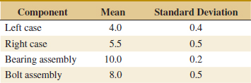
(a) What is the probability that the weight of an assembly exceeds 29.5 ounces?
(b) What is the probability that the mean weight of eight independent assemblies exceeds 29 ounces?
5-115. Suppose that X and Y have a bivariate normal distribution with σX = 4, σY = 1, /, μY = 4, and ρ = −0.2. Draw a rough contour plot of the joint probability density function.
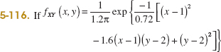
determine E(X), E(Y) V(X), V(Y), and ρ by reorganizing the parameters in the joint probability density function.
5-117. ![]() The permeability of a membrane used as a moisture barrier in a biological application depends on the thickness of two integrated layers. The layers are normally distributed with means of 0.5 and 1 millimeters, respectively. The standard deviations of layer thickness are 0.1 and 0.2 millimeters, respectively. The correlation between layers is 0.7.
The permeability of a membrane used as a moisture barrier in a biological application depends on the thickness of two integrated layers. The layers are normally distributed with means of 0.5 and 1 millimeters, respectively. The standard deviations of layer thickness are 0.1 and 0.2 millimeters, respectively. The correlation between layers is 0.7.
(a) Determine the mean and variance of the total thickness of the two layers.
(b) What is the probability that the total thickness is less than 1 millimeter?
(c) Let X1 and X2 denote the thickness of layers 1 and 2, respectively. A measure of performance of the membrane is a function of 2X1 + 3X2 of the thickness. Determine the mean and variance of this performance measure.
5-118. ![]() The permeability of a membrane used as a moisture barrier in a biological application depends on the thickness of three integrated layers. Layers 1, 2, and 3 are normally distributed with means of 0.5, 1, and 1.5 millimeters, respectively. The standard deviations of layer thickness are 0.1, 0.2, and 0.3, respectively. Also, the correlation between layers 1 and 2 is 0.7, between layers 2 and 3 is 0.5, and between layers 1 and 3 is 0.3.
The permeability of a membrane used as a moisture barrier in a biological application depends on the thickness of three integrated layers. Layers 1, 2, and 3 are normally distributed with means of 0.5, 1, and 1.5 millimeters, respectively. The standard deviations of layer thickness are 0.1, 0.2, and 0.3, respectively. Also, the correlation between layers 1 and 2 is 0.7, between layers 2 and 3 is 0.5, and between layers 1 and 3 is 0.3.
(a) Determine the mean and variance of the total thickness of the three layers.
(b) What is the probability that the total thickness is less than 1.5 millimeters?
5-119. A small company is to decide what investments to use for cash generated from operations. Each investment has a mean and standard deviation associated with the percentage gain. The first security has a mean percentage gain of 5% with a standard deviation of 2%, and the second security provides the same mean of 5% with a standard deviation of 4%. The securities have a correlation of –0.5, so there is a negative correlation between the percentage returns. If the company invests two million dollars with half in each security, what are the mean and standard deviation of the percentage return? Compare the standard deviation of this strategy to one that invests the two million dollars into the first security only.
5-120. ![]() An order of 15 printers contains 4 with a graphics-enhancement feature, 5 with extra memory, and 6 with both features. Four printers are selected at random, without replacement, from this set. Let the random variables X, Y, and Z denote the number of printers in the sample with graphics enhancement only, extra memory only, and both, respectively.
An order of 15 printers contains 4 with a graphics-enhancement feature, 5 with extra memory, and 6 with both features. Four printers are selected at random, without replacement, from this set. Let the random variables X, Y, and Z denote the number of printers in the sample with graphics enhancement only, extra memory only, and both, respectively.
(a) Describe the range of the joint probability distribution of X, Y, and Z.
(b) Is the probability distribution of X, Y, and Z multinomial? Why or why not?
(c) Determine the conditional probability distribution of X given that Y = 2.
Determine the following:
(d) P(X = 1, Y = 2, Z = 1)
(e) P(X = 1, Y = 1)
(f) E(X) and V(X)
(g) P(X = 1, Y = 2|Z = 1)
(h) P(X = 2|Y = 2)
(i) Conditional probability distribution of X given that Y = 0 and Z = 3.
5-121. ![]() A marketing company performed a risk analysis for a manufacturer of synthetic fibers and concluded that new competitors present no risk 13% of the time (due mostly to the diversity of fibers manufactured), moderate risk 72% of the time (some overlapping of products), and very high risk (competitor manufactures the exact same products) 15% of the time. It is known that 12 international companies are planning to open new facilities for the manufacture of synthetic fibers within the next three years. Assume that the companies are independent. Let X, Y, and Z denote the number of new competitors that will pose no, moderate, and very high risk for the interested company, respectively.
A marketing company performed a risk analysis for a manufacturer of synthetic fibers and concluded that new competitors present no risk 13% of the time (due mostly to the diversity of fibers manufactured), moderate risk 72% of the time (some overlapping of products), and very high risk (competitor manufactures the exact same products) 15% of the time. It is known that 12 international companies are planning to open new facilities for the manufacture of synthetic fibers within the next three years. Assume that the companies are independent. Let X, Y, and Z denote the number of new competitors that will pose no, moderate, and very high risk for the interested company, respectively.
Determine the following:
(a) Range of the joint probability distribution of X, Y, and Z
(b) P(X = 1, Y = 3, Z = 1)
(c) P(Z ≤ 2)
(d) P(Z = 2|Y = 1, X = 10)
(e) P(Z ≤ 1|X = 10)
(f) P(Y ≤ 1, Z ≤ 1|X = 10)
(g) E(Z|X = 10)
5-122. Suppose X has a lognormal distribution with parameters θ and ω. Determine the probability density function and the parameters values for Y = Xγ for a constant γ > 0. What is the name of this distribution?
5-123. The power in a DC circuit is P = I2/R where I and R denote the current and resistance, respectively. Suppose that I is normally distributed with mean of 200 mA and standard deviation 0.2 mA and R is a constant. Determine the probability density function of power.
5-124. The intensity (mW/mm2) of a laser beam on a surface theoretically follows a bivariate normal distribution with maximum intensity at the center, equal variance σ in the x and y directions, and zero covariance. There are several definitions for the width of the beam. One definition is the diameter at which the intensity is 50% of its peak. Suppose that the beam width is 1.6 mm under this definition. Determine σ. Also determine the beam width when it is defined as the diameter where the intensity equals 1/e2 of the peak.
5-125. Use moment generating functions to determine the normalized power [E(X4)]¼ from a cycling power meter when X has a normal distribution with mean 200 and standard deviation 20 Watts.
5-126. Show that if X1, X2,..., Xp are independent, continuous random variables, P(X1 ∈ A1, X2 ∈ A2,..., Xp ∈ Ap) = P(X1 ∈ A1)P(X2 ∈ A2). . .P(Xp ∈ Ap) for any regions A1, A2,..., Ap in the range of X1, X2,..., Xp respectively.
5-127. Show that if X1, X2,..., Xp are independent random variables and Y = c1X1 + c2X2 + . . . + cpXp, V(Y) = ![]() (X1) +
(X1) + ![]() (X2) + . . . +
(X2) + . . . + ![]() (Xp)
(Xp)
You may assume that the random variables are continuous.
5-128. Suppose that the joint probability function of the continuous random variables X and Y is constant on the rectangle 0 < x < a, 0 < y < b. Show that X and Y are independent.
5-129. Suppose that the range of the continuous variables X and Y is 0 < x < a and 0 < y < b. Also suppose that the joint probability density function fXY(x, y) = g(x)h(y), where g(x) is a function only of x, and h(y) is a function only of y. Show that X and Y are independent.
5-130. This exercise extends the hypergeometric distribution to multiple variables. Consider a population with N items of k different types. Assume that there are N1 items of type 1, N2 items of type 2,..., Nk items of type k so that N1 + N2 + . . . + . . .Nk = N. Suppose that a random sample of size n is selected, without replacement, from the population. Let X1, X2,..., Xk denote the number of items of each type in the sample so that X1 + X2, + . . . + . . . + Xk = n. Show that for feasible values of n, x1, x2,..., xk, N1, N2,..., Nk, the probability is
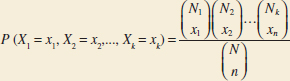
5-131. Use the properties of moment generating functions to show that a sum of p independent normal random variables with means μi and variances ![]() for i = 1,2,. . .p has a normal distribution.
for i = 1,2,. . .p has a normal distribution.
5-132. Show that by expanding etX in a power series and taking expectations term by term we may write the moment-generating function as
![]()
Thus, the coefficient of tr/r! in this expansion is μ′r, the rth origin moment.
Write the power series expansion for MX(t) for a gamma random variable and determine μ′1 and μ′2 using this approach.
Important Terms and Concepts
Bivariate distribution
Bivariate normal distribution
Conditional mean
Conditional probability
density function
Conditional probability mass function
Conditional variance
Contour plots
Correlation
Covariance
Error propagation
General functions of random variables
Independence
Joint probability density function
Joint probability distribution
Joint probability mass function
Linear functions of random variables
Marginal probability distribution
Moment generating functions
Multinomial distribution
Reproductive property of the normal distribution