

Simple Linear Regression and Correlation

Chapter Outline
11-3 Properties of the Least Squares Estimators
11-4 Hypothesis Tests in Simple Linear Regression
11-4.2 Analysis of Variance Approach to Test Significance of Regression
11-5.1 Confidence Intervals on the Slope and Intercept
11-5.2 Confidence Interval on the Mean Response
11-6 Prediction of New Observations
11-7 Adequacy of the Regression Model
11-7.2 Coefficient of Determination (R2)
The space shuttle Challenger accident in January 1986 was the result of the failure of O-rings used to seal field joints in the solid rocket motor because of the extremely low ambient temperatures at the time of launch. Prior to the launch, there were data on the occurrence of O-ring failure and the corresponding temperature on 24 prior launches or static firings of the motor. In this chapter, we will see how to build a statistical model relating the probability of O-ring failure to temperature. This model provides a measure of the risk associated with launching the shuttle at the low temperature when Challenger was launched.
After careful study of this chapter, you should be able to do the following:
- Use simple linear regression for building empirical models to engineering and scientific data
- Understand how the method of least squares is used to estimate the parameters in a linear regression model
- Analyze residuals to determine whether the regression model is an adequate fit to the data or whether any underlying assumptions are violated
- Test statistical hypotheses and construct confidence intervals on regression model parameters
- Use the regression model to predict a future observation and ctoonstruct an appropriate prediction interval on the future observation
- Apply the correlation model
- Use simple transformations to achieve a linear regression model
11-1 Empirical Models
Many problems in engineering and the sciences involve a study or analysis of the relationship between two or more variables. For example, the pressure of a gas in a container is related to the temperature, the velocity of water in an open channel is related to the width of the channel, and the displacement of a particle at a certain time is related to its velocity. In this last example, if we let d0 be the displacement of the particle from the origin at time t = 0 and v be the velocity, the displacement at time t is dt = d0 + vt. This is an example of a deterministic linear relationship because (apart from measurement errors) the model predicts displacement perfectly.
However, in many situations, the relationship between variables is not deterministic. For example, the electrical energy consumption of a house (y) is related to the size of the house (x, in square feet), but it is unlikely to be a deterministic relationship. Similarly, the fuel usage of an automobile (y) is related to the vehicle weight x, but the relationship is not a deterministic one. In both of these examples, the value of the response of interest y (energy consumption, fuel usage) cannot be predicted perfectly from knowledge of the corresponding x. It is possible for different automobiles to have different fuel usage even if they weigh the same, and it is possible for different houses to use different amounts of electricity even if they are the same size.
The collection of statistical tools that are used to model and explore relationships between variables that are related in a nondeterministic manner is called regression analysis. Because problems of this type occur so frequently in many branches of engineering and science, regression analysis is one of the most widely used statistical tools. In this chapter, we present the situation in which there is only one independent or predictor variable x and the relationship with the response y is assumed to be linear. Although this seems to be a simple scenario, many practical problems fall into this framework.
For example, in a chemical process, suppose that the yield of the product is related to the process-operating temperature. Regression analysis can be used to build a model to predict yield at a given temperature level. This model can also be used for process optimization, such as finding the level of temperature that maximizes yield, or for process control purposes.
As an illustration, consider the data in Table 11-1. In this table, y is the purity of oxygen produced in a chemical distillation process, and x is the percentage of hydrocarbons present in the main condenser of the distillation unit. Figure 11-1 presents a scatter diagram of the data in Table 11-1. This is just a graph on which each (xi, yi) pair is represented as a point plotted in a two-dimensional coordinate system. This scatter diagram was produced by a computer, and we selected an option that shows dot diagrams of the x and y variables along the top and right margins of the graph, respectively, making it easy to see the distributions of the individual variables (box plots or histograms could also be selected). Inspection of this scatter diagram indicates that, although no simple curve will pass exactly through all the points, there is a strong indication that the points lie scattered randomly around a straight line. Therefore, it is probably reasonable to assume that the mean of the random variable Y is related to x by the following straight-line relationship:
![]()
where the slope and intercept of the line are called regression coefficients. Although the mean of Y is a linear function of x, the actual observed value y does not fall exactly on a straight line. The appropriate way to generalize this to a probabilistic linear model is to assume that the expected value of Y is a linear function of x but that for a fixed value of x, the actual value of Y is determined by the mean value function (the linear model) plus a random error term, say,
![]()
Simple Linear Regression Model
where ![]() is the random error term. We will call this model the simple linear regression model because it has only one independent variable or regressor. Sometimes a model like this arises from a theoretical relationship. At other times, we will have no theoretical knowledge of the relationship between x and y and will base the choice of the model on inspection of a scatter diagram, such as we did with the oxygen purity data. We then think of the regression model as an empirical model.
is the random error term. We will call this model the simple linear regression model because it has only one independent variable or regressor. Sometimes a model like this arises from a theoretical relationship. At other times, we will have no theoretical knowledge of the relationship between x and y and will base the choice of the model on inspection of a scatter diagram, such as we did with the oxygen purity data. We then think of the regression model as an empirical model.
To gain more insight into this model, suppose that we can fix the value of x and observe the value of the random variable Y. Now if x is fixed, the random component ![]() on the right-hand side of the model in Equation 11-1 determines the properties of Y. Suppose that the mean and variance of
on the right-hand side of the model in Equation 11-1 determines the properties of Y. Suppose that the mean and variance of ![]() are 0 and σ2, respectively. Then,
are 0 and σ2, respectively. Then,
![]()
![]() TABLE • 11-1 Oxygen and Hydrocarbon Levels
TABLE • 11-1 Oxygen and Hydrocarbon Levels

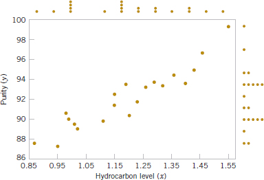
FIGURE 11-1 Scatter diagram of oxygen purity versus hydrocarbon level from Table 11-1.
Notice that this is the same relationship that we initially wrote down empirically from inspection of the scatter diagram in Fig. 11-1. The variance of Y given x is
![]()
Thus, the true regression model μY|x = β0 + β1x is a line of mean values; that is, the height of the regression line at any value of x is just the expected value of Y for that x. The slope, β1, can be interpreted as the change in the mean of Y for a unit change in x. Furthermore, the variability of Y at a particular value of x is determined by the error variance σ2. This implies that there is a distribution of Y-values at each x and that the variance of this distribution is the same at each x.
For example, suppose that the true regression model relating oxygen purity to hydrocarbon level is μY|x = 75 + 15x, and suppose that the variance is σ2 = 2. Figure 11-2 illustrates this situation. Notice that we have used a normal distribution to describe the random variation in σ2. Because σ2 is the sum of a constant β0 + β1x (the mean) and a normally distributed random variable, Y is a normally distributed random variable. The variance σ2 determines the variability in the observations Y on oxygen purity. Thus, when σ2 is small, the observed values of Y will fall close to the line, and when σ2 is large, the observed values of Y may deviate considerably from the line. Because σ2 is constant, the variability in Y at any value of x is the same.
The regression model describes the relationship between oxygen purity Y and hydrocarbon level x. Thus, for any value of hydrocarbon level, oxygen purity has a normal distribution with mean 75 + 15x and variance 2. For example, if x = 1.25, Y has mean value μY|x = 75 + 15(1.25) = 93.75 and variance 2.
In most real-world problems, the values of the intercept and slope (β0, β1) and the error variance σ2 will not be known and must be estimated from sample data. Then this fitted regression equation or model is typically used in prediction of future observations of Y, or for estimating the mean response at a particular level of x. To illustrate, a chemical engineer might be interested in estimating the mean purity of oxygen produced when the hydrocarbon level is x = 1.25%. This chapter discusses such procedures and applications for the simple linear regression model. Chapter 12 will discuss multiple linear regression models that involve more than one regressor.
Historical Note
Sir Francis Galton first used the term regression analysis in a study of the heights of fathers (x) and sons (y). Galton fit a least squares line and used it to predict the son's height from the father's height. He found that if a father's height was above average, the son's height would also be above average but not by as much as the father's height was. A similar effect was observed for below average heights. That is, the son's height “regressed” toward the average. Consequently, Galton referred to the least squares line as a regression line.

FIGURE 11-2 The distribution of Y for a given value of x for the oxygen purity-hydrocarbon data.
Abuses of Regression
Regression is widely used and frequently misused; we mention several common abuses of regression briefly here. Care should be taken in selecting variables with which to construct regression equations and in determining the form of the model. It is possible to develop statistically significant relationships among variables that are completely unrelated in a causal sense. For example, we might attempt to relate the shear strength of spot welds with the number of empty parking spaces in the visitor parking lot. A straight line may even appear to provide a good fit to the data, but the relationship is an unreasonable one on which to rely. We cannot increase the weld strength by blocking off parking spaces. A strong observed association between variables does not necessarily imply that a causal relationship exists between them. This type of effect is encountered fairly often in retrospective data analysis and even in observational studies. Designed experiments are the only way to determine cause-and-effect relationships.
Regression relationships are valid for values of the regressor variable only within the range of the original data. The linear relationship that we have tentatively assumed may be valid over the original range of x, but it may be unlikely to remain so as we extrapolate—that is, if we use values of x beyond that range. In other words, as we move beyond the range of values of R2 for which data were collected, we become less certain about the validity of the assumed model. Regression models are not necessarily valid for extrapolation purposes.
Now this does not mean do not ever extrapolate. For many problem situations in science and engineering, extrapolation of a regression model is the only way to even approach the problem. However, there is a strong warning to be careful. A modest extrapolation may be perfectly all right in many cases, but a large extrapolation will almost never produce acceptable results.
11-2 Simple Linear Regression
The case of simple linear regression considers a single regressor variable or predictor variable x and a dependent or response variable Y. Suppose that the true relationship between Y and x is a straight line and that the observation Y at each level of x is a random variable. As noted previously, the expected value of Y for each value of x is
![]()
where the intercept β0 and the slope β1 are unknown regression coefficients. We assume that each observation, Y, can be described by the model
![]()
where ![]() is a random error with mean zero and (unknown) variance σ2. The random errors corresponding to different observations are also assumed to be uncorrelated random variables.
is a random error with mean zero and (unknown) variance σ2. The random errors corresponding to different observations are also assumed to be uncorrelated random variables.
Suppose that we have n pairs of observations (x1, y1),(x2, y2),...,(xn, yn). Figure 11-3 is a typical scatter plot of observed data and a candidate for the estimated regression line. The estimates of β0 and β1 should result in a line that is (in some sense) a “best fit” to the data. The German scientist Karl Gauss (1777–1855) proposed estimating the parameters β0 and β1 in Equation 11-2 to minimize the sum of the squares of the vertical deviations in Fig. 11-3.
We call this criterion for estimating the regression coefficients the method of least squares. Using Equation 11-2, we may express the n observations in the sample as
![]()
and the sum of the squares of the deviations of the observations from the true regression line is
![]()
The least squares estimators of β0 and β1, say, ![]() 0 and
0 and ![]() 1, must satisfy
1, must satisfy

Simplifying these two equations yields

Equations 11-6 are called the least squares normal equations. The solution to the normal equations results in the least squares estimators ![]() 0 and
0 and ![]() 1.
1.
Least Squares Estimates
The least squares estimates of the intercept and slope in the simple linear regression model are
![]()

where ![]() and
and ![]() .
.
The fitted or estimated regression line is therefore
![]()
Note that each pair of observations satisfies the relationship
![]()
where ei = yi − ![]() i is called the residual. The residual describes the error in the fit of the model to the ith observation yi. Later in this chapter, we will use the residuals to provide information about the adequacy of the fitted model.
i is called the residual. The residual describes the error in the fit of the model to the ith observation yi. Later in this chapter, we will use the residuals to provide information about the adequacy of the fitted model.

FIGURE 11-3 Deviations of the data from the estimated regression model.
Notationally, it is occasionally convenient to give special symbols to the numerator and denominator of Equation 11-8. Given data (x1, y1),(x2, y2),...,(xn, yn), let

and

Example 11-1 Oxygen Purity We will fit a simple linear regression model to the oxygen purity data in Table 11-1. The following quantities may be computed:

and

Therefore, the least squares estimates of the slope and intercept are
![]()
and
![]()
The fitted simple linear regression model (with the coefficients reported to three decimal places) is
![]()
This model is plotted in Fig. 11-4, along with the sample data.
Practical Interpretation: Using the regression model, we would predict oxygen purity of ![]() = 89.23% when the hydrocarbon level is x = 1.00%. The 89.23% purity may be interpreted as an estimate of the true population mean purity when x = 1.00%, or as an estimate of a new observation when x = 1.00%. These estimates are, of course, subject to error; that is, it is unlikely that a future observation on purity would be exactly 89.23% when the hydrocarbon level is 1.00%. In subsequent sections, we will see how to use confidence intervals and prediction intervals to describe the error in estimation from a regression model.
= 89.23% when the hydrocarbon level is x = 1.00%. The 89.23% purity may be interpreted as an estimate of the true population mean purity when x = 1.00%, or as an estimate of a new observation when x = 1.00%. These estimates are, of course, subject to error; that is, it is unlikely that a future observation on purity would be exactly 89.23% when the hydrocarbon level is 1.00%. In subsequent sections, we will see how to use confidence intervals and prediction intervals to describe the error in estimation from a regression model.
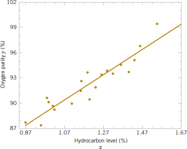
FIGURE 11-4 Scatter plot of oxygen purity y versus hydrocarbon level x and regression model ![]() = 74.283 + 14.947x.
= 74.283 + 14.947x.
Computer software programs are widely used in regression modeling. These programs typically carry more decimal places in the calculations. See Table 11-2 for a portion of typical output from a software package for this problem. The estimates ![]() 0 and
0 and ![]() 1 are highlighted. In subsequent sections, we will provide explanations for the information provided in this computer output.
1 are highlighted. In subsequent sections, we will provide explanations for the information provided in this computer output.
![]() TABLE • 11-2 Software Output for the Oxygen Purity Data in Example 11-1
TABLE • 11-2 Software Output for the Oxygen Purity Data in Example 11-1

Estimating σ2
There is actually another unknown parameter in our regression model, σ2 (the variance of the error term ![]() ). The residuals ei = yi −
). The residuals ei = yi − ![]() i are used to obtain an estimate of σ2. The sum of squares of the residuals, often called the error sum of squares, is
i are used to obtain an estimate of σ2. The sum of squares of the residuals, often called the error sum of squares, is
![]()
We can show that the expected value of the error sum of squares is E(SSE) = (n − 2)σ2. Therefore, an unbiased estimator of σ2 is
Estimator of Variance
![]()
Computing SSE using Equation 11-12 would be fairly tedious. A more convenient computing formula can be obtained by substituting ![]() i =
i = ![]() 0 +
0 + ![]() 1xi into Equation 11-12 and simplifying. The resulting computing formula is
1xi into Equation 11-12 and simplifying. The resulting computing formula is
![]()
where SST = ![]() (yi −
(yi − ![]() )2 =
)2 = ![]() is the total sum of squares of the response variable y. Formulas such as this are presented in Section 11-4. The error sum of squares and the estimate of σ2 for the oxygen purity data,
is the total sum of squares of the response variable y. Formulas such as this are presented in Section 11-4. The error sum of squares and the estimate of σ2 for the oxygen purity data, ![]() 2 = 1.18, are highlighted in the computer output in Table 11-2.
2 = 1.18, are highlighted in the computer output in Table 11-2.
Exercises FOR SECTION 11-2
![]() Problem available in WileyPLUS at instructor's discretion.
Problem available in WileyPLUS at instructor's discretion.
![]() Go Tutorial Tutoring problem available in WileyPLUS at instructor's discretion.
Go Tutorial Tutoring problem available in WileyPLUS at instructor's discretion.
11-1. Diabetes and obesity are serious health concerns in the United States and much of the developed world. Measuring the amount of body fat a person carries is one way to monitor weight control progress, but measuring it accurately involves either expensive X-ray equipment or a pool in which to dunk the subject. Instead body mass index (BMI) is often used as a proxy for body fat because it is easy to measure: BMI = mass (kg)/(height (m))2 = 703 mass(lb)/(height(in))2. In a study of 250 men at Bingham Young University, both BMI and body fat were measured. Researchers found the following summary statistics:

(a) ![]() Calculate the least squares estimates of the slope and intercept. Graph the regression line.
Calculate the least squares estimates of the slope and intercept. Graph the regression line.
(b) ![]() Use the equation of the fitted line to predict what body fat would be observed, on average, for a man with a BMI of 30.
Use the equation of the fitted line to predict what body fat would be observed, on average, for a man with a BMI of 30.
(c) Suppose that the observed body fat of a man with a BMI of 25 is 25%. Find the residual for that observation.
(d) Was the prediction for the BMI of 25 in part (c) an overestimate or underestimate? Explain briefly.
11-2. On average, do people gain weight as they age? Using data from the same study as in Exercise 11-1, we provide some summary statistics for both age and weight.

(a) Calculate the least squares estimates of the slope and intercept. Graph the regression line.
(b) Use the equation of the fitted line to predict the weight that would be observed, on average, for a man who is 25 years old.
(c) Suppose that the observed weight of a 25-year-old man is 170 lbs. Find the residual for that observation.
(d) Was the prediction for the 25-year-old in part (c) an overestimate or underestimate? Explain briefly.

11-3. ![]() An article in Concrete Research [“Near Surface Characteristics of Concrete: Intrinsic Permeability” (1989, Vol. 41)] presented data on compressive strength x and intrinsic permeability y of various concrete mixes and cures. Summary quantities are n = 14,
An article in Concrete Research [“Near Surface Characteristics of Concrete: Intrinsic Permeability” (1989, Vol. 41)] presented data on compressive strength x and intrinsic permeability y of various concrete mixes and cures. Summary quantities are n = 14, ![]() = 572,
= 572, ![]() = 23,530,
= 23,530, ![]() = 43,
= 43, ![]() = 157.42, and
= 157.42, and ![]() = 1697.80. Assume that the two variables are related according to the simple linear regression model.
= 1697.80. Assume that the two variables are related according to the simple linear regression model.
(a) Calculate the least squares estimates of the slope and intercept. Estimate σ2. Graph the regression line.
(b) Use the equation of the fitted line to predict what permeability would be observed when the compressive strength is x = 4.3.
(c) Give a point estimate of the mean permeability when compressive strength is x = 3.7.
(d) Suppose that the observed value of permeability at x = 3.7 is y = 46.1. Calculate the value of the corresponding residual.
11-4. ![]() Regression methods were used to analyze the data from a study investigating the relationship between roadway surface temperature (x) and pavement deflection (y). Summary quantities were n = 20,
Regression methods were used to analyze the data from a study investigating the relationship between roadway surface temperature (x) and pavement deflection (y). Summary quantities were n = 20, ![]() = 12.75,
= 12.75, ![]() = 8.86,
= 8.86, ![]() = 1478,
= 1478, ![]() = 143,215.8, and
= 143,215.8, and ![]() = 1083.67.
= 1083.67.
(a) Calculate the least squares estimates of the slope and intercept. Graph the regression line. Estimate σ2.
(b) Use the equation of the fitted line to predict what pavement deflection would be observed when the surface temperature is 85°F.
(c) What is the mean pavement deflection when the surface temperature is 90°F?
(d) What change in mean pavement deflection would be expected for a 1°F change in surface temperature?
![]()
11-5. ![]() See Table E11-1 for data on the ratings of quarter-backs for the 2008 National Football League season (The Sports Network). It is suspected that the rating (y) is related to the average number of yards gained per pass attempt (x).
See Table E11-1 for data on the ratings of quarter-backs for the 2008 National Football League season (The Sports Network). It is suspected that the rating (y) is related to the average number of yards gained per pass attempt (x).
(a) Calculate the least squares estimates of the slope and intercept. What is the estimate of σ2? Graph the regression model.
(b) Find an estimate of the mean rating if a quarterback averages 7.5 yards per attempt.
(c) What change in the mean rating is associated with a decrease of one yard per attempt?
(d) To increase the mean rating by 10 points, how much increase in the average yards per attempt must be generated?
(e) Given that x = 7.21 yards, find the fitted value of x and the corresponding residual.
![]()
11-6. ![]() An article in Technometrics by S. C. Narula and J. F. Wellington [“Prediction, Linear Regression, and a Minimum Sum of Relative Errors” (1977, Vol. 19)] presents data on the selling price and annual taxes for 24 houses. The data are in the Table E11-2.
An article in Technometrics by S. C. Narula and J. F. Wellington [“Prediction, Linear Regression, and a Minimum Sum of Relative Errors” (1977, Vol. 19)] presents data on the selling price and annual taxes for 24 houses. The data are in the Table E11-2.
(a) Assuming that a simple linear regression model is appropriate, obtain the least squares fit relating selling price to taxes paid. What is the estimate of σ2?
(b) Find the mean selling price given that the taxes paid are x = 7.50.

(c) Calculate the fitted value of y corresponding to x = 5.8980. Find the corresponding residual.
(d) Calculate the fitted ![]() i for each value of xi used to fit the model. Then construct a graph of
i for each value of xi used to fit the model. Then construct a graph of ![]() i versus the corresponding observed value yi and comment on what this plot would look like if the relationship between y and x was a deterministic (no random error) straight line. Does the plot actually obtained indicate that taxes paid is an effective regressor variable in predicting selling price?
i versus the corresponding observed value yi and comment on what this plot would look like if the relationship between y and x was a deterministic (no random error) straight line. Does the plot actually obtained indicate that taxes paid is an effective regressor variable in predicting selling price?
![]() 11-7. The number of pounds of steam used per month by a chemical plant is thought to be related to the average ambient temperature (in °F) for that month. The past year's usage and temperatures are in the following table:
11-7. The number of pounds of steam used per month by a chemical plant is thought to be related to the average ambient temperature (in °F) for that month. The past year's usage and temperatures are in the following table:

(a) Assuming that a simple linear regression model is appropriate, fit the regression model relating steam usage (y) to the average temperature (x). What is the estimate of σ2? Graph the regression line.
(b) What is the estimate of expected steam usage when the average temperature is 55°F?
(c) What change in mean steam usage is expected when the monthly average temperature changes by 1°F?
(d) Suppose that the monthly average temperature is 47°F. Calculate the fitted value of y and the corresponding residual.
![]()
11-8. ![]() Go Tutorial Table E11-3 presents the highway gasoline mileage performance and engine displacement for DaimlerChrysler vehicles for model year 2005 (U.S. Environmental Protection Agency).
Go Tutorial Table E11-3 presents the highway gasoline mileage performance and engine displacement for DaimlerChrysler vehicles for model year 2005 (U.S. Environmental Protection Agency).
(a) Fit a simple linear model relating highway miles per gallon (y) to engine displacement (x) in cubic inches using least squares.
(b) Find an estimate of the mean highway gasoline mileage performance for a car with 150 cubic inches engine displacement.
(c) Obtain the fitted value of y and the corresponding residual for a car, the Neon, with an engine displacement of 122 cubic inches.
![]()
11-9. An article in the Tappi Journal (March 1986) presented data on green liquor Na2S concentration (in grams per liter) and paper machine production (in tons per day). The data (read from a graph) follow:

(a) Fit a simple linear regression model with y = green liquor Na2S concentration and x = production. Find an estimate of σ2. Draw a scatter diagram of the data and the resulting least squares fitted model.
(b) Find the fitted value of y corresponding to x = 910 and the associated residual.
(c) Find the mean green liquor Na2S concentration when the production rate is 950 tons per day.
![]()
11-10. An article in the Journal of Sound and Vibration (1991, Vol. 151, pp. 383–394) described a study investigating the relationship between noise exposure and hypertension. The following data are representative of those reported in the article.

(a) Draw a scatter diagram of y (blood pressure rise in millimeters of mercury) versus x (sound pressure level in decibels). Does a simple linear regression model seem reasonable in this situation?
(b) Fit the simple linear regression model using least squares. Find an estimate of σ2.
(c) Find the predicted mean rise in blood pressure level associated with a sound pressure level of 85 decibels.
11-11. An article in Wear (1992, Vol. 152, pp. 171–181) presents data on the fretting wear of mild steel and oil viscosity. Representative data follow with x = oil viscosity and y = wear volume (10−4 cubic millimeters).
![]() TABLE • E11-3 Gasoline Mileage Data
TABLE • E11-3 Gasoline Mileage Data


(a) Construct a scatter plot of the data. Does a simple linear regression model appear to be plausible?
(b) Fit the simple linear regression model using least squares. Find an estimate of σ2.
(c) Predict fretting wear when viscosity x = 30.
(d) Obtain the fitted value of y when x = 22.0 and calculate the corresponding residual.
![]()
11-12. ![]() An article in the Journal of Environmental Engineering (1989, Vol. 115(3), pp. 608–619) reported the results of a study on the occurrence of sodium and chloride in surface streams in central Rhode Island. The following data are chloride concentration y (in milligrams per liter) and roadway area in the watershed x (in percentage).
An article in the Journal of Environmental Engineering (1989, Vol. 115(3), pp. 608–619) reported the results of a study on the occurrence of sodium and chloride in surface streams in central Rhode Island. The following data are chloride concentration y (in milligrams per liter) and roadway area in the watershed x (in percentage).
(a) Draw a scatter diagram of the data. Does a simple linear regression model seem appropriate here?
(b) Fit the simple linear regression model using the method of least squares. Find an estimate of σ2.
(c) Estimate the mean chloride concentration for a watershed that has 1% roadway area.
(d) Find the fitted value corresponding to x = 0.47 and the associated residual.
![]()
11-13. A rocket motor is manufactured by bonding together two types of propellants, an igniter and a sustainer. The shear strength of the bond y is thought to be a linear function of the age of the propellant x when the motor is cast. Table E11-4 provides 20 observations.
(a) Draw a scatter diagram of the data. Does the straight-line regression model seem to be plausible?
(b) Find the least squares estimates of the slope and intercept in the simple linear regression model. Find an estimate of σ2.
(c) Estimate the mean shear strength of a motor made from propellant that is 20 weeks old.
(d) Obtain the fitted values ![]() i that correspond to each observed value yi. Plot
i that correspond to each observed value yi. Plot ![]() i versus yi and comment on what this plot would look like if the linear relationship between shear strength and age were perfectly deterministic (no error). Does this plot indicate that age is a reasonable choice of regressor variable in this model?
i versus yi and comment on what this plot would look like if the linear relationship between shear strength and age were perfectly deterministic (no error). Does this plot indicate that age is a reasonable choice of regressor variable in this model?
![]()
11-14. ![]() Go Tutorial An article in the Journal of the American Ceramic Society [“Rapid Hot-Pressing of Ultrafine PSZ Powders” (1991, Vol. 74, pp. 1547–1553)] considered the microstructure of the ultrafine powder of partially stabilized zirconia as a function of temperature. The data follow:
Go Tutorial An article in the Journal of the American Ceramic Society [“Rapid Hot-Pressing of Ultrafine PSZ Powders” (1991, Vol. 74, pp. 1547–1553)] considered the microstructure of the ultrafine powder of partially stabilized zirconia as a function of temperature. The data follow:


(a) Fit the simple linear regression model using the method of least squares. Find an estimate of σ2.
(b) Estimate the mean porosity for a temperature of 1400°C.
(c) Find the fitted value corresponding to y = 11.4 and the associated residual.
(d) Draw a scatter diagram of the data. Does a simple linear regression model seem appropriate here? Explain.
![]() 11-15.
11-15. ![]() An article in the Journal of the Environmental Engineering Division [“Least Squares Estimates of BOD Parameters” (1980, Vol. 106, pp. 1197–1202)] took a sample from the Holston River below Kingport, Tennessee, during August 1977. The biochemical oxygen demand (BOD) test is conducted over a period of time in days. The resulting data follow:
An article in the Journal of the Environmental Engineering Division [“Least Squares Estimates of BOD Parameters” (1980, Vol. 106, pp. 1197–1202)] took a sample from the Holston River below Kingport, Tennessee, during August 1977. The biochemical oxygen demand (BOD) test is conducted over a period of time in days. The resulting data follow:

(a) Assuming that a simple linear regression model is appropriate, fit the regression model relating BOD (y) to the time (x). What is the estimate of σ2?
(b) What is the estimate of expected BOD level when the time is 15 days?
(c) What change in mean BOD is expected when the time changes by three days?
(d) Suppose that the time used is six days. Calculate the fitted value of y and the corresponding residual.
(e) Calculate the fitted ![]() i for each value of xi used to fit the model. Then construct a graph of
i for each value of xi used to fit the model. Then construct a graph of ![]() i versus the corresponding observed values yi and comment on what this plot would look like if the relationship between y and x was a deterministic (no random error) straight line. Does the plot actually obtained indicate that time is an effective regressor variable in predicting BOD?
i versus the corresponding observed values yi and comment on what this plot would look like if the relationship between y and x was a deterministic (no random error) straight line. Does the plot actually obtained indicate that time is an effective regressor variable in predicting BOD?
![]()
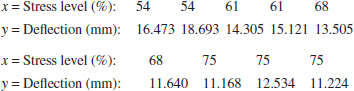
11-16. An article in Wood Science and Technology [“Creep in Chipboard, Part 3: Initial Assessment of the Influence of Moisture Content and Level of Stressing on Rate of Creep and Time to Failure” (1981, Vol. 15, pp. 125–144)] reported a study of the deflection (mm) of particleboard from stress levels of relative humidity. Assume that the two variables are related according to the simple linear regression model. The data follow:
(a) Calculate the least square estimates of the slope and intercept. What is the estimate of σ2? Graph the regression model and the data.
(b) Find the estimate of the mean deflection if the stress level can be limited to 65%.
(c) Estimate the change in the mean deflection associated with a 5% increment in stress level.
(d) To decrease the mean deflection by one millimeter, how much increase in stress level must be generated?
(e) Given that the stress level is 68%, find the fitted value of deflection and the corresponding residual.
![]()
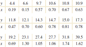
11-17. In an article in Statistics and Computing [“An Iterative Monte Carlo Method for Nonconjugate Bayesian Analysis” (1991, pp. 119–128)], Carlin and Gelfand investigated the age (x) and length (y) of 27 captured dugongs (sea cows).

(a) Find the least squares estimates of the slope and the intercept in the simple linear regression model. Find an estimate of σ2.
(b) Estimate the mean length of dugongs at age 11.
(c) Obtain the fitted values ![]() i that correspond to each observed value yi. Plot
i that correspond to each observed value yi. Plot ![]() i versus yi, and comment on what this plot would look like if the linear relationship between length and age were perfectly deterministic (no error). Does this plot indicate that age is a reasonable choice of regressor variable in this model?
i versus yi, and comment on what this plot would look like if the linear relationship between length and age were perfectly deterministic (no error). Does this plot indicate that age is a reasonable choice of regressor variable in this model?
11-18. Consider the regression model developed in Exercise 11-4.
(a) Suppose that temperature is measured in °C rather than °F. Write the new regression model.
(b) What change in expected pavement deflection is associated with a 1°C change in surface temperature?
11-19. ![]() Consider the regression model developed in Exercise 11-8. Suppose that engine displacement is measured in cubic centimeters instead of cubic inches.
Consider the regression model developed in Exercise 11-8. Suppose that engine displacement is measured in cubic centimeters instead of cubic inches.
(a) Write the new regression model.
(b) What change in gasoline mileage is associated with a 1 cm3 change is engine displacement?
11-20. Show that in a simple linear regression model the point (![]() ,
, ![]() ) lies exactly on the least squares regression line.
) lies exactly on the least squares regression line.
![]()
11-21. ![]() Consider the simple linear regression model Y = β0 + β1x +
Consider the simple linear regression model Y = β0 + β1x + ![]() . Suppose that the analyst wants to use z = x −
. Suppose that the analyst wants to use z = x − ![]() as the regressor variable.
as the regressor variable.
(a) Using the data in Exercise 11-13, construct one scatter plot of the (xi, yi) points and then another of the (zi = xi − ![]() , yi) points. Use the two plots to intuitively explain how the two models, Y = β0 + β1x +
, yi) points. Use the two plots to intuitively explain how the two models, Y = β0 + β1x + ![]() and Y =
and Y = ![]() z +
z + ![]() , are related.
, are related.
(b) Find the least squares estimates of ![]() and
and ![]() in the model Y =
in the model Y = ![]() +
+ ![]() . How do they relate to the least squares estimates
. How do they relate to the least squares estimates ![]() 0 and
0 and ![]() 1?
1?
![]()
11-22. Suppose that we wish to fit a regression model for which the true regression line passes through the point (0, 0). The appropriate model is Y = βx + ![]() . Assume that we have n pairs of data (x1, y1), (x2, y2),...,(xn, yn).
. Assume that we have n pairs of data (x1, y1), (x2, y2),...,(xn, yn).
(a) Find the least squares estimate of β.
(b) Fit the model Y = βx + ![]() to the chloride concentration-roadway area data in Exercise 11-12. Plot the fitted model on a scatter diagram of the data and comment on the appropriateness of the model.
to the chloride concentration-roadway area data in Exercise 11-12. Plot the fitted model on a scatter diagram of the data and comment on the appropriateness of the model.
11-3 Properties of the Least Squares Estimators
The statistical properties of the least squares estimators ![]() 0 and
0 and ![]() 1 may be easily described. Recall that we have assumed that the error term
1 may be easily described. Recall that we have assumed that the error term ![]() in the model Y = β0 + β1x +
in the model Y = β0 + β1x + ![]() is a random variable with mean zero and variance σ2. Because the values of x are fixed, Y is a random variable with mean μY|x = β0 + β1x and variance σ2. Therefore, the values of
is a random variable with mean zero and variance σ2. Because the values of x are fixed, Y is a random variable with mean μY|x = β0 + β1x and variance σ2. Therefore, the values of ![]() 0 and
0 and ![]() 1 depend on the observed y's; thus, the least squares estimators of the regression coefficients may be viewed as random variables. We will investigate the bias and variance properties of the least squares estimators
1 depend on the observed y's; thus, the least squares estimators of the regression coefficients may be viewed as random variables. We will investigate the bias and variance properties of the least squares estimators ![]() 0 and
0 and ![]() 1.
1.
Consider first ![]() 1. Because
1. Because ![]() 1 is a linear combination of the observations Yi, we can use properties of expectation to show that the expected value of
1 is a linear combination of the observations Yi, we can use properties of expectation to show that the expected value of ![]() 1 is
1 is
![]()
Thus, ![]() 1 is an unbiased estimator in simple linear regression of the true slope β1.
1 is an unbiased estimator in simple linear regression of the true slope β1.
Now consider the variance of ![]() 1. Because we have assumed that V(
1. Because we have assumed that V(![]() i) = σ2, it follows that V(Yi) = σ2. Because
i) = σ2, it follows that V(Yi) = σ2. Because ![]() 1 is a linear combination of the observations Yi, the results in Section 5-5 can be applied to show that
1 is a linear combination of the observations Yi, the results in Section 5-5 can be applied to show that
![]()
For the intercept, we can show in a similar manner that
![]()
Thus, ![]() 0 is an unbiased estimator of the intercept β0. The covariance of the random variables
0 is an unbiased estimator of the intercept β0. The covariance of the random variables ![]() 0 and
0 and ![]() 1 is not zero. It can be shown (see Exercise 11-110) that cov(
1 is not zero. It can be shown (see Exercise 11-110) that cov(![]() 0,
0, ![]() 1) = −σ2
1) = −σ2![]() /Sxx.
/Sxx.
The estimate of σ2 could be used in Equations 11-16 and 11-17 to provide estimates of the variance of the slope and the intercept. We call the square roots of the resulting variance estimators the estimated standard errors of the slope and intercept, respectively.
In simple linear regression, the estimated standard error of the slope and the estimated standard error of the intercept are

respectively, where ![]() 2 is computed from Equation 11-13.
2 is computed from Equation 11-13.
The computer output in Table 11-2 reports the estimated standard errors of the slope and intercept under the column heading SE coeff.
11-4 Hypothesis Tests in Simple Linear Regression
An important part of assessing the adequacy of a linear regression model is testing statistical hypotheses about the model parameters and constructing certain confidence intervals. Hypothesis testing in simple linear regression is discussed in this section, and Section 11-5 presents methods for constructing confidence intervals. To test hypotheses about the slope and intercept of the regression model, we must make the additional assumption that the error component in the model, ![]() , is normally distributed. Thus, the complete assumptions are that the errors are normally and independently distributed with mean zero and variance σ2, abbreviated NID(0, σ2).
, is normally distributed. Thus, the complete assumptions are that the errors are normally and independently distributed with mean zero and variance σ2, abbreviated NID(0, σ2).
11-4.1 USE OF t-TESTS
Suppose that we wish to test the hypothesis that the slope equals a constant, say, β1,0. The appropriate hypotheses are
![]()
where we have assumed a two-sided alternative. Because the errors ![]() i are NID(0, σ2), it follows directly that the observations Yi are NID(β0 + β1xi, σ2). Now
i are NID(0, σ2), it follows directly that the observations Yi are NID(β0 + β1xi, σ2). Now ![]() 1 is a linear combination of independent normal random variables, and consequently,
1 is a linear combination of independent normal random variables, and consequently, ![]() 1 is N(β1, σ2/Sxx), using the bias and variance properties of the slope discussed in Section 11-3. In addition, (n − 2)
1 is N(β1, σ2/Sxx), using the bias and variance properties of the slope discussed in Section 11-3. In addition, (n − 2)![]() 2/σ2 has a chi-square distribution with n − 2 degrees of freedom, and
2/σ2 has a chi-square distribution with n − 2 degrees of freedom, and ![]() 1 is independent of
1 is independent of ![]() 2. As a result of those properties, the statistic
2. As a result of those properties, the statistic
Test Statistic for the slope

follows the t distribution with n − 2 degrees of freedom under H0:β1 = β1,0. We would reject H0:β1 = β1,0 if
![]()
where t0 is computed from Equation 11-19. The denominator of Equation 11-19 is the standard error of the slope, so we could write the test statistic as

A similar procedure can be used to test hypotheses about the intercept. To test
![]()
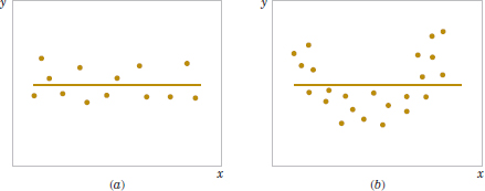
FIGURE 11-5 The hypothesis H0:β1 = 0 is not rejected.
we would use the statistic
Test Statistic for the Intercept

and reject the null hypothesis if the computed value of this test statistic, t0, is such that |t0| > tα/2,n−2. Note that the denominator of the test statistic in Equation 11-22 is just the standard error of the intercept.
A very important special case of the hypotheses of Equation 11-18 is
![]()
These hypotheses relate to the significance of regression. Failure to reject H0:β1 = 0 is equivalent to concluding that there is no linear relationship between x and Y. This situation is illustrated in Fig. 11-5. Note that this may imply either that x is of little value in explaining the variation in Y and that the best estimator of Y for any x is ![]() =
= ![]() [Fig. 11-5(a)] or that the true relationship between x and Y is not linear [Fig. 11-5(b)]. Alternatively, if H0: β1 = 0 is rejected, this implies that x is of value in explaining the variability in Y (see Fig. 11-6). Rejecting H0: β1 = 0 could mean either that the straight-line model is adequate [Fig. 11-6(a)] or that, although there is a linear effect of x, better results could be obtained with the addition of higher order polynomial terms in x [Fig. 11-6(b)].
[Fig. 11-5(a)] or that the true relationship between x and Y is not linear [Fig. 11-5(b)]. Alternatively, if H0: β1 = 0 is rejected, this implies that x is of value in explaining the variability in Y (see Fig. 11-6). Rejecting H0: β1 = 0 could mean either that the straight-line model is adequate [Fig. 11-6(a)] or that, although there is a linear effect of x, better results could be obtained with the addition of higher order polynomial terms in x [Fig. 11-6(b)].
Example 11-2 Oxygen Purity Tests of Coefficients We will test for significance of regression using the model for the oxygen purity data from Example 11-1. The hypotheses are
![]()
and we will use α = 0.01. From Example 11-1 and Table 11-2 we have
![]()
so the t-statistic in Equation 10-20 becomes

Practical Interpretation: Because the reference value of t is t0.005,18 = 2.88, the value of the test statistic is very far into the critical region, implying that H0: β1 = 0 should be rejected. There is strong evidence to support this claim. The P-value for this test is P ![]() 1.23 × 10− 9. This was obtained manually with a calculator.
1.23 × 10− 9. This was obtained manually with a calculator.
Table 11-2 presents the typical computer output for this problem. Notice that the t-statistic value for the slope is computed as 11.35 and that the reported P-value is P = 0.000. The computer also reports the t-statistic for testing the hypothesis H0: β0 = 0. This statistic is computed from Equation 11-22, with β0.0 = 0, as t0 = 46.62. Clearly, then, the hypothesis that the intercept is zero is rejected.

FIGURE 11-6 The hypothesis H0:β1 = 0 is rejected.
11-4.2 ANALYSIS OF VARIANCE APPROACH TO TEST SIGNIFICANCE OF REGRESSION
A method called the analysis of variance can be used to test for significance of regression. The procedure partitions the total variability in the response variable into meaningful components as the basis for the test. The analysis of variance identity is as follows:
Analysis of Variance Identity

The two components on the right-hand-side of Equation 11-24 measure, respectively, the amount of variability in yi accounted for by the regression line and the residual variation left unexplained by the regression line. We usually call SSE = ![]() (yi −
(yi − ![]() i)2 the error sum of squares and SSE =
i)2 the error sum of squares and SSE = ![]() (
(![]() −
− ![]() )2 the regression sum of squares. Symbolically, Equation 11-24 may be written as
)2 the regression sum of squares. Symbolically, Equation 11-24 may be written as
![]()
where SST = ![]() (yi −
(yi − ![]() )2 is the total corrected sum of squares of y. In Section 11-2, we noted that SSE = SST −
)2 is the total corrected sum of squares of y. In Section 11-2, we noted that SSE = SST − ![]() 1Sxy (see Equation 11-14), so because SST =
1Sxy (see Equation 11-14), so because SST = ![]() 1Sxy + SSE, we note that the regression sum of squares in Equation 11-25 is SSR =
1Sxy + SSE, we note that the regression sum of squares in Equation 11-25 is SSR = ![]() 1Sxy. The total sum of squares SST has n − 1 degrees of freedom, and SSR and SSE have 1 and n − 2 degrees of freedom, respectively.
1Sxy. The total sum of squares SST has n − 1 degrees of freedom, and SSR and SSE have 1 and n − 2 degrees of freedom, respectively.
We may show that E[SSE/(n − 2)] = σ2 and E(SSR) = σ2 + ![]() and that SSE/σ2 and SSR/σ2 are independent chi-square random variables with n − 2 and 1 degrees of freedom, respectively. Thus, if the null hypothesis H0: β1 = 0 is true, the statistic
and that SSE/σ2 and SSR/σ2 are independent chi-square random variables with n − 2 and 1 degrees of freedom, respectively. Thus, if the null hypothesis H0: β1 = 0 is true, the statistic
Test for Significance of Regression

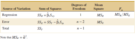
follows the F1,n−2 distribution, and we would reject H0 if f0 > fα,1,n−2. The quantities MSR = SSR/1 and MSE = SSE/(n − 2) are called mean squares. In general, a mean square is always computed by dividing a sum of squares by its number of degrees of freedom. The test procedure is usually arranged in an analysis of variance table, such as Table 11-3.
![]() TABLE • 11-3 Analysis of Variance for Testing Significance of Regression
TABLE • 11-3 Analysis of Variance for Testing Significance of Regression
Example 11-3 Oxygen Purity ANOVA We will use the analysis of variance approach to test for significance of regression using the oxygen purity data model from Example 11-1. Recall that SST = 173.38, ![]() 1 = 14.947, Sxy = 10.17744, and n = 20. The regression sum of squares is
1 = 14.947, Sxy = 10.17744, and n = 20. The regression sum of squares is
![]()
and the error sum of squares is
![]()
The analysis of variance for testing H0: β1 = 0 is summarized in the computer output in Table 11-2. The test statistic is f0 = MSR/MSE = 152.13/1.18 = 128.86, for which we find that the P-value is P ![]() 1.23 × 10⁻⁹, so we conclude that β1 is not zero.
1.23 × 10⁻⁹, so we conclude that β1 is not zero.
Frequently computer packages have minor differences in terminology. For example, sometimes the regression sum of squares is called the “model” sum of squares, and the error sum of squares is called the “residual” sum of squares.
Note that the analysis of variance procedure for testing for significance of regression is equivalent to the t-test in Section 11-4.1. That is, either procedure will lead to the same conclusions. This is easy to demonstrate by starting with the t-test statistic in Equation 11-19 with β1,0 = 0, say
![]()
Squaring both sides of Equation 11-27 and using the fact that ![]() 2 = MSE results in
2 = MSE results in
![]()
Note that ![]() in Equation 11-28 is identical to F0 in Equation 11-26. It is true, in general, that the square of a t random variable with v degrees of freedom is an F random variable with 1 and v degrees of freedom in the numerator and denominator, respectively. Thus, the test using T0 is equivalent to the test based on F0. Note, however, that the t-test is somewhat more flexible in that it would allow testing against a one-sided alternative hypothesis, while the F-test is restricted to a two-sided alternative.
in Equation 11-28 is identical to F0 in Equation 11-26. It is true, in general, that the square of a t random variable with v degrees of freedom is an F random variable with 1 and v degrees of freedom in the numerator and denominator, respectively. Thus, the test using T0 is equivalent to the test based on F0. Note, however, that the t-test is somewhat more flexible in that it would allow testing against a one-sided alternative hypothesis, while the F-test is restricted to a two-sided alternative.
![]() Problem available in WileyPLUS at instructor's discretion.
Problem available in WileyPLUS at instructor's discretion.
![]() Go Tutorial Tutoring problem available in WileyPLUS at instructor's discretion.
Go Tutorial Tutoring problem available in WileyPLUS at instructor's discretion.
11-23. ![]() Recall the regression of percent body fat on BMI from Exercise 11-1.
Recall the regression of percent body fat on BMI from Exercise 11-1.
(a) Estimate the error standard deviation.
(b) Estimate the standard deviation of the slope.
(c) What is the value of the t-statistic for the slope?
(d) Test the hypothesis that β1 = 0 at α = 0.05. What is the P-value for this test?
11-24. ![]() Recall the regression of weight on age from Exercise 11-2.
Recall the regression of weight on age from Exercise 11-2.
(a) Estimate the error standard deviation.
(b) Estimate the standard deviation of the slope.
(c) What is the value of the t-statistic for the slope?
(d) Test the hypothesis that β1 = 0 at α = 0.05. What is the P-value for this test?
11-25. Suppose that in Exercise 11-24 weight is measured in kg instead of lbs.
(a) How will the estimates of the slope and intercept change?
(b) Estimate the error standard deviation.
(c) Estimate the standard deviation of the slope.
(d) What is the value of the t-statistic for the slope? Compare your answer to the one for Exercise 11-24(c).
(e) Test the hypothesis that β1 = 0 at α = 0.05. What is the P-value for this test? Compare your answer to the one for Exercise 11-24(d). Comment briefly.
11-26. Consider the simple linear regression model y = 10 + 25x + ε where the random error term is normally and independently distributed with mean zero and standard deviation 2. Use software to generate a sample of eight observations, one each at the levels x = 10, 12, 14, 16, 18, 20, 22, and 24.
(a) Fit the linear regression model by least squares and find the estimates of the slope and intercept.
(b) Find the estimate of σ2.
(c) Find the standard errors of the slope and intercept.
(d) Now use software to generate a sample of 16 observations, two each at the same levels of x used previously. Fit the model using least squares.
(e) Find the estimate of σ2 for the new model in part (d). Compare this to the estimate obtained in part (b). What impact has the increase in sample size had on the estimate?
(f) Find the standard errors of the slope and intercept using the new model from part (d). Compare these standard errors to the ones that you found in part (c). What impact has the increase in sample size had on the estimated standard errors?
11-27. ![]() Consider the following computer output.
Consider the following computer output.

(a) Fill in the missing information. You may use bounds for the P-values.
(b) Can you conclude that the model defines a useful linear relationship?
(c) What is your estimate of σ2?
11-28. ![]() Consider the following computer output.
Consider the following computer output.

(a) Fill in the missing information. You may use bounds for the P-values.
(b) Can you conclude that the model defines a useful linear relationship?
(c) What is your estimate of σ2?
11-29. Consider the data from Exercise 11-3 on x = compressive strength and y = intrinsic permeability of concrete.
(a) Test for significance of regression using α = 0.05. Find the P-value for this test. Can you conclude that the model specifies a useful linear relationship between these two variables?
(b) Estimate σ2 and the standard deviation of ![]() 1.
1.
(c) What is the standard error of the intercept in this model?
11-30. ![]() Go Tutorial Consider the data from Exercise 11-4 on x = roadway surface temperature and y = pavement deflection.
Go Tutorial Consider the data from Exercise 11-4 on x = roadway surface temperature and y = pavement deflection.
(a) Test for significance of regression using α = 0.05. Find the P-value for this test. What conclusions can you draw?
(b) Estimate the standard errors of the slope and intercept.
![]() 11-31.
11-31. ![]() Consider the National Football League data in Exercise 11-5.
Consider the National Football League data in Exercise 11-5.
(a) Test for significance of regression using α = 0.01. Find the P-value for this test. What conclusions can you draw?
(b) Estimate the standard errors of the slope and intercept.
(c) Test H0: β1 = 10 versus H1: β1 ≠ 10 with α = 0.01. Would you agree with the statement that this is a test of the hypothesis that a one-yard increase in the average yards per attempt results in a mean increase of 10 rating points?
![]() 11-32. Consider the data from Exercise 11-6 on y = sales price and x = taxes paid.
11-32. Consider the data from Exercise 11-6 on y = sales price and x = taxes paid.
(a) Test H0: β1 = 0 using the t-test; use α = 0.05.
(b) Test H0: β1 = 0 using the analysis of variance with α = 0.05. Discuss the relationship of this test to the test from part (a).
(c) Estimate the standard errors of the slope and intercept.
(d) Test the hypothesis that β0 = 0.
![]() 11-33. Consider the data from Exercise 11-7 on y = steam usage and x = average temperature.
11-33. Consider the data from Exercise 11-7 on y = steam usage and x = average temperature.
(a) Test for significance of regression using α = 0.01. What is the P-value for this test? State the conclusions that result from this test.
(b) Estimate the standard errors of the slope and intercept.
(c) Test the hypothesis H0: β1 = 10 versus H1: β1 ≠ 10 using α = 0.01. Find the P-value for this test.
(d) Test H0: β0 = 0 versus H0: β0 ≠ 0 using α = 0.01. Find the P-value for this test and draw conclusions.
![]() 11-34.
11-34. ![]() Consider the data from Exercise 11-8 on y = highway gasoline mileage and x = engine displacement.
Consider the data from Exercise 11-8 on y = highway gasoline mileage and x = engine displacement.
(a) Test for significance of regression using α = 0.01. Find the P-value for this test. What conclusions can you reach?
(b) Estimate the standard errors of the slope and intercept.
(c) Test H0:β1 = −0.05 versus H1:β1 < −0.05 using α = 0.01 and draw conclusions. What is the P-value for this test?
(d) Test the hypothesis H0: β0 = 0 versus H1: β0 ≠ 0 using α = 0.01. What is the P-value for this test?
![]() 11-35. Consider the data from Exercise 11-9 on y = green liquor Na2S concentration and x = production in a paper mill.
11-35. Consider the data from Exercise 11-9 on y = green liquor Na2S concentration and x = production in a paper mill.
(a) Test for significance of regression using α = 0.05. Find the P-value for this test.
(b) Estimate the standard errors of the slope and intercept.
(c) Test H0: β0 = 0 versus H1: β0 ≠ 0 using α = 0.05. What is the P-value for this test?
![]() 11-36. Consider the data from Exercise 11-10 on y = blood pressure rise and x = sound pressure level.
11-36. Consider the data from Exercise 11-10 on y = blood pressure rise and x = sound pressure level.
(a) Test for significance of regression using α = 0.05. What is the P-value for this test?
(b) Estimate the standard errors of the slope and intercept.
(c) Test H0: β0 = 0 versus H1: β0 ≠ 0 using α = 0.05. Find the P-value for this test.
![]()
11-37. ![]() Consider the data from Exercise 11-13, on y = shear strength of a propellant and x = propellant age.
Consider the data from Exercise 11-13, on y = shear strength of a propellant and x = propellant age.
(a) Test for significance of regression with α = 0.01. Find the P-value for this test.
(b) Estimate the standard errors of ![]() 0 and
0 and ![]() 1.
1.
(c) Test H0: β1 = −30 versus H1: β1 ≠ −30 using α = 0.01. What is the P-value for this test?
(d) Test H0: β0 = 0 versus H1: β0 ≠ 0 using α = 0.01. What is the P-value for this test?
(e) Test H0: β0 = 2500 versus H1: β0 > 2500 using α = 0.01. What is the P-value for this test?
![]()
11-38. Consider the data from Exercise 11-12 on y = chloride concentration in surface streams and x = roadway area.
(a) Test the hypothesis H0: β1 = 0 versus H1: β1 ≠ 0 using the analysis of variance procedure with α = 0.01.
(b) Find the P-value for the test in part (a).
(c) Estimate the standard errors of ![]() 1 and
1 and ![]() 0.
0.
(d) Test H0: β1 = 0 versus H1: β0 ≠ 0 using α = 0.01. What conclusions can you draw? Does it seem that the model might be a better fit to the data if the intercept were removed?
![]()
11-39. ![]() Consider the data in Exercise 11-15 on y = oxygen demand and x = time.
Consider the data in Exercise 11-15 on y = oxygen demand and x = time.
(a) Test for significance of regression using α = 0.01. Find the P-value for this test. What conclusions can you draw?
(b) Estimate the standard errors of the slope and intercept.
(c) Test the hypothesis that β0 = 0.
![]()
11-40. ![]() Consider the data in Exercise 11-16 on y = deflection and x = stress level.
Consider the data in Exercise 11-16 on y = deflection and x = stress level.
(a) Test for significance of regression using α = 0.01. What is the P-value for this test? State the conclusions that result from this test.
(b) Does this model appear to be adequate?
(c) Estimate the standard errors of the slope and intercept.
![]()
11-41. ![]() Go Tutorial An article in The Journal of Clinical Endocrinology and Metabolism [“Simultaneous and Continuous 24-Hour Plasma and Cerebrospinal Fluid Leptin Measurements: Dissociation of Concentrations in Central and Peripheral Compartments” (2004, Vol. 89, pp. 258–265)] reported on a study of the demographics of simultaneous and continuous 24-hour plasma and cerebrospinal fluid leptin measurements. The data follow:
Go Tutorial An article in The Journal of Clinical Endocrinology and Metabolism [“Simultaneous and Continuous 24-Hour Plasma and Cerebrospinal Fluid Leptin Measurements: Dissociation of Concentrations in Central and Peripheral Compartments” (2004, Vol. 89, pp. 258–265)] reported on a study of the demographics of simultaneous and continuous 24-hour plasma and cerebrospinal fluid leptin measurements. The data follow:

(a) Test for significance of regression using α = 0.05. Find the P-value for this test. Can you conclude that the model specifies a useful linear relationship between these two variables?
(b) Estimate σ2 and the standard deviation of ![]() 1.
1.
(c) What is the standard error of the intercept in this model?
11-42. ![]() Suppose that each value of xi is multiplied by a positive constant a, and each value of yi is multiplied by another positive constant b. Show that the t-statistic for testing H0: β1 = 0 versus H1: β1 ≠ 0 is unchanged in value.
Suppose that each value of xi is multiplied by a positive constant a, and each value of yi is multiplied by another positive constant b. Show that the t-statistic for testing H0: β1 = 0 versus H1: β1 ≠ 0 is unchanged in value.
11-43. ![]() The type II error probability for the t-test for H0: β1 = β1,0 can be computed in a similar manner to the t-tests of Chapter 9. If the true value of β1 is β′1, the value d = |β1,0 − β′1|/(σ
The type II error probability for the t-test for H0: β1 = β1,0 can be computed in a similar manner to the t-tests of Chapter 9. If the true value of β1 is β′1, the value d = |β1,0 − β′1|/(σ![]() is calculated and used as the horizontal scale factor on the operating characteristic curves for the t-test (Appendix Charts VIIe through VIIh) and the type II error probability is read from the vertical scale using the curve for n − 2 degrees of freedom. Apply this procedure to the football data in Exercise 11-3, using σ = 5.5 and β′1 = 12.5 where the hypotheses are H0: β1 = 10 versus H0: β1 ≠ 10.
is calculated and used as the horizontal scale factor on the operating characteristic curves for the t-test (Appendix Charts VIIe through VIIh) and the type II error probability is read from the vertical scale using the curve for n − 2 degrees of freedom. Apply this procedure to the football data in Exercise 11-3, using σ = 5.5 and β′1 = 12.5 where the hypotheses are H0: β1 = 10 versus H0: β1 ≠ 10.
11-44. ![]() Consider the no-intercept model Y = βx +
Consider the no-intercept model Y = βx + ![]() with the
with the ![]() 's NID (0, σ2). The estimate of σ2 is s2 =
's NID (0, σ2). The estimate of σ2 is s2 = ![]() (yi −
(yi − ![]() xi)2/(n − 1) and V(
xi)2/(n − 1) and V(![]() ) = σ2/
) = σ2/![]() .
.
(a) Devise a test statistic for H0: β = 0 versus H1: β ≠ 0.
(b) Apply the test in (a) to the model from Exercise 11-22.
11-5 Confidence Intervals
11-5.1 CONFIDENCE INTERVALS ON THE SLOPE AND INTERCEPT
In addition to point estimates of the slope and intercept, it is possible to obtain confidence interval estimates of these parameters. The width of these confidence intervals is a measure of the overall quality of the regression line. If the error terms, ![]() i, in the regression model are normally and independently distributed,
i, in the regression model are normally and independently distributed,

are both distributed as t random variables with n − 2 degrees of freedom. This leads to the following definition of 100(1 − α)% confidence intervals on the slope and intercept.
Confidence Intervals on Parameters
Under the assumption that the observations are normally and independently distributed, a 100(1 − α)% confidence interval on the slope β1 in simple linear regression is
![]()
Similarly, a 100(1 − α)% confidence interval on the intercept β0 is

Example 11-4 Oxygen Purity Confidence Interval on the Slope We will find a 95% confidence interval on the slope of the regression line using the data in Example 11-1. Recall that ![]() 1 = 14.947, Sxx = 0.68088, and
1 = 14.947, Sxx = 0.68088, and ![]() 2 = 1.18 (see Table 11-2). Then, from Equation 11-29, we find
2 = 1.18 (see Table 11-2). Then, from Equation 11-29, we find
![]()
or
![]()
This simplifies to
![]()
Practical Interpretation: This CI does not include zero, so there is strong evidence (at α = 0.05) that the slope is not zero. The CI is reasonably narrow (± 2.766) because the error variance is fairly small.
11-5.2 CONFIDENCE INTERVAL ON THE MEAN RESPONSE
A confidence interval may be constructed on the mean response at a specified value of x, say, x0. This is a confidence interval about E(Y|x0) = μY|x0 and is sometimes referred to as a confidence interval about the regression line. Because E(Y|x0) = μY|x0 = β0 + β1x0, we may obtain a point estimate of the mean of Y at x = x0(μY|x0) from the fitted model as
![]()
Now ![]() Y|x0 is an unbiased point estimator of μY|x0 because
Y|x0 is an unbiased point estimator of μY|x0 because ![]() 0 and
0 and ![]() 1 are unbiased estimators of β0 and β1. The variance of
1 are unbiased estimators of β0 and β1. The variance of ![]() Y|x0 is
Y|x0 is
![]()
This last result follows from the fact that ![]() Y|x0 =
Y|x0 = ![]() +
+ ![]() 1(x0 −
1(x0 − ![]() ) and cov (
) and cov (![]() ,
, ![]() 1) = 0. The zero covariance result is left as a mind-expanding exercise. Also,
1) = 0. The zero covariance result is left as a mind-expanding exercise. Also, ![]() Y|x0 is normally distributed because
Y|x0 is normally distributed because ![]() 1 and
1 and ![]() 0 are normally distributed, and if we use
0 are normally distributed, and if we use ![]() 2 as an estimate of σ2, it is easy to show that
2 as an estimate of σ2, it is easy to show that

has a t distribution with n − 2 degrees of freedom. This leads to the following confidence interval definition.
Confidence Interval on the Mean Response
A 100(1 − α)% confidence interval on the mean response at the value of x = x0, say μY|x0, is given by
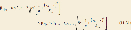
where ![]() is computed from the fitted regression model.
is computed from the fitted regression model.
Note that the width of the CI for μY|x0 is a function of the value specified for x0. The interval width is a minimum for x0 = ![]() and widens as |x0 −
and widens as |x0 − ![]() | increases.
| increases.
Example 11-5 Oxygen Purity Confidence Interval on the Mean Response We will construct a 95% confidence interval about the mean response for the data in Example 11-1. The fitted model is ![]() Y|x0 = 74.283 + 14.947x0, and the 95% confidence interval on μY|x0 is found from Equation 11-31 as
Y|x0 = 74.283 + 14.947x0, and the 95% confidence interval on μY|x0 is found from Equation 11-31 as

Suppose that we are interested in predicting mean oxygen purity when x0 = 1.00%. Then
![]()
and the 95% confidence interval is

or
![]()
Therefore, the 95% CI on μY|1.00 is
![]()
This is a reasonably narrow CI.
Most computer software will also perform these calculations. Refer to Table 11-2. The predicted value of y at x = 1.00 is shown along with the 95% CI on the mean of y at this level of x.
By repeating these calculations for several different values for x0, we can obtain confidence limits for each corresponding value of μY|x0. Figure 11-7 is a display of the scatter diagram with the fitted model and the corresponding 95% confidence limits plotted as the upper and lower lines. The 95% confidence level applies only to the interval obtained at one value of x, not to the entire set of x-levels. Notice that the width of the confidence interval on μY|x0 increases as |x0 − ![]() | increases.
| increases.
11-6 Prediction of New Observations
An important application of a regression model is predicting new or future observations Y corresponding to a specified level of the regressor variable x. If x0 is the value of the regressor variable of interest,
![]()
is the point estimator of the new or future value of the response Y0.
Now consider obtaining an interval estimate for this future observation Y0. This new observation is independent of the observations used to develop the regression model. Therefore, the confidence interval for μY|x0 in Equation 11-31 is inappropriate because it is based only on the data used to fit the regression model. The confidence interval about μY|x0 refers to the true mean response at x = x0 (that is, a population parameter), not to future observations.

FIGURE 11-7 Scatter diagram of oxygen purity data from Example 11-1 with fitted regression line and 95 percent confidence limits on μY|x0.
Let Y0 be the future observation at x = x0, and let ![]() 0 given by Equation 11-32 be the estimator of Y0. Note that the error in prediction
0 given by Equation 11-32 be the estimator of Y0. Note that the error in prediction
![]()
is a normally distributed random variable with mean zero and variance
![]()
because Y0 is independent of ![]() 0. If we use
0. If we use ![]() 2 to estimate σ2, we can show that
2 to estimate σ2, we can show that

has a t distribution with n − 2 degrees of freedom. From this, we can develop the following prediction interval definition.
Prediction Interval
A 100(1 − α)% prediction interval on a future observation Y0 at the value x0 is given by

The value ![]() 0 is computed from the regression model
0 is computed from the regression model ![]() 0 =
0 = ![]() 0 +
0 + ![]() 1x0.
1x0.
Notice that the prediction interval is of minimum width at x0 = ![]() and widens as |x0 −
and widens as |x0 − ![]() | increases. By comparing Equation 11-33 with Equation 11-31, we observe that the prediction interval at the point x0 is always wider than the confidence interval at x0. This results because the prediction interval depends on both the error from the fitted model and the error associated with future observations.
| increases. By comparing Equation 11-33 with Equation 11-31, we observe that the prediction interval at the point x0 is always wider than the confidence interval at x0. This results because the prediction interval depends on both the error from the fitted model and the error associated with future observations.
Example 11-6 Oxygen Purity Prediction Interval To illustrate the construction of a prediction interval, suppose that we use the data in Example 11-1 and find a 95% prediction interval on the next observation of oxygen purity at x0 = 1.00%. Using Equation 11-33 and recalling from Example 11-5 that ![]() 0 = 89.23, we find that the prediction interval is
0 = 89.23, we find that the prediction interval is

which simplifies to
![]()
This is a reasonably narrow prediction interval.
Typical computer software will also calculate prediction intervals. Refer to the output in Table 11-2. The 95% PI on the future observation at x0 = 1.00 is shown in the display.
By repeating the foregoing calculations at different levels of x0, we may obtain the 95% prediction intervals shown graphically as the lower and upper lines about the fitted regression model in Fig. 11-8. Notice that this graph also shows the 95% confidence limits on μY|x0 calculated in Example 11-5. It illustrates that the prediction limits are always wider than the confidence limits.

FIGURE 11-8 Scatter diagram of oxygen purity data from Example 11-1 with fitted regression line, 95% prediction limits (outer lines), and 95% confidence limits on μY|x0.
Exercises FOR SECTIONS 11-5 AND 11-6
![]() Problem available in WileyPLUS at instructor's discretion.
Problem available in WileyPLUS at instructor's discretion.
![]() Go Tutorial Tutoring problem available in WileyPLUS at instructor's discretion.
Go Tutorial Tutoring problem available in WileyPLUS at instructor's discretion.
11-45. ![]() Using the regression from Exercise 11-1,
Using the regression from Exercise 11-1,
(a) Find a 95% confidence interval for the slope.
(b) Find a 95% confidence interval for the mean percent body fat for a man with a BMI of 25.
(c) Find a 95% prediction interval for the percent body fat for a man with a BMI of 25.
(d) Which interval is wider, the confidence interval or the prediction interval? Explain briefly.
11-46. ![]() Using the regression from Exercise 11-2,
Using the regression from Exercise 11-2,
(a) Find a 95% confidence interval for the slope.
(b) Find a 95% confidence interval for the mean weight for a man 25 years old.
(c) Find a 95% prediction interval for the weight of a 25 year old man.
(d) Which interval is wider, the confidence interval or the prediction interval? Explain briefly.
(e) Without using age, find a 95% confidence interval for the mean weight of all men. Compare this to the interval in part (b).
11-47. ![]() Refer to the data in Exercise 11-3 on y = intrinsic permeability of concrete and x = compressive strength. Find a 95% confidence interval on each of the following:
Refer to the data in Exercise 11-3 on y = intrinsic permeability of concrete and x = compressive strength. Find a 95% confidence interval on each of the following:
(a) Slope
(b) Intercept
(c) Mean permeability when x = 2.5
(d) Find a 95% prediction interval on permeability when x = 2.5. Explain why this interval is wider than the interval in part (c).
11-48. ![]() Exercise 11-4 presented data on roadway surface temperature x and pavement deflection y. Find a 99% confidence interval on each of the following:
Exercise 11-4 presented data on roadway surface temperature x and pavement deflection y. Find a 99% confidence interval on each of the following:
(a) Slope
(b) Intercept
(c) Mean deflection when temperature x = 85°F
(d) Find a 99% prediction interval on pavement deflection when the temperature is 90°F.
![]() 11-49. Refer to the NFL quarterback ratings data in Exercise 11-5. Find a 95% confidence interval on each of the following:
11-49. Refer to the NFL quarterback ratings data in Exercise 11-5. Find a 95% confidence interval on each of the following:
(a) Slope
(b) Intercept
(c) Mean rating when the average yards per attempt is 8.0
(d) Find a 95% prediction interval on the rating when the average yards per attempt is 8.0.
![]() 11-50.
11-50. ![]() Refer to the data on y = house selling price and x = taxes paid in Exercise 11-6. Find a 95% confidence interval on each of the following:
Refer to the data on y = house selling price and x = taxes paid in Exercise 11-6. Find a 95% confidence interval on each of the following:
(a) β1
(b) β0
(c) Mean selling price when the taxes paid are x = 7.50
(d) Compute the 95% prediction interval for selling price when the taxes paid are x = 7.50.
![]() 11-51. Exercise 11-7 presented data on y = steam usage and x = monthly average temperature.
11-51. Exercise 11-7 presented data on y = steam usage and x = monthly average temperature.
(a) Find a 99% confidence interval for β1.
(b) Find a 99% confidence interval for β0.
(c) Find a 95% confidence interval on mean steam usage when the average temperature is 55°F.
(d) Find a 95% prediction interval on steam usage when temperature is 55°F. Explain why this interval is wider than the interval in part (c).
![]() 11-52. Exercise 11-8 presented gasoline mileage performance for 21 cars along with information about the engine displacement. Find a 95% confidence interval on each of the following:
11-52. Exercise 11-8 presented gasoline mileage performance for 21 cars along with information about the engine displacement. Find a 95% confidence interval on each of the following:
(a) Slope
(b) Intercept
(c) Mean highway gasoline mileage when the engine displacement is x = 150 in3
(d) Construct a 95% prediction interval on highway gasoline mileage when the engine displacement is x = 150 in3.
![]() 11-53.
11-53. ![]() Consider the data in Exercise 11-9 on y = green liquor Na2S concentration and x = production in a paper mill. Find a 99% confidence interval on each of the following:
Consider the data in Exercise 11-9 on y = green liquor Na2S concentration and x = production in a paper mill. Find a 99% confidence interval on each of the following:
(a) β1
(b) β0
(c) Mean Na2S concentration when production x = 910 tons/day
(d) Find a 99% prediction interval on Na2S concentration when x = 910 tons/day.
![]()
11-54. Exercise 11-10 presented data on y = blood pressure rise and x = sound pressure level. Find a 95% confidence interval on each of the following:
(a) β1
(b) β0
(c) Mean blood pressure rise when the sound pressure level is 85 decibels
(d) Find a 95% prediction interval on blood pressure rise when the sound pressure level is 85 decibels.
![]()
11-55. ![]() Refer to the data in Exercise 11-11 on y = wear volume of mild steel and x = oil viscosity. Find a 95% confidence interval on each of the following:
Refer to the data in Exercise 11-11 on y = wear volume of mild steel and x = oil viscosity. Find a 95% confidence interval on each of the following:
(a) Intercept
(b) Slope
(c) Mean wear when oil viscosity x = 30
![]()
11-56. Exercise 11-12 presented data on chloride concentration y and roadway area x on watersheds in central Rhode Island. Find a 99% confidence interval on each of the following:
(a) β1
(b) β0
(c) Mean chloride concentration when roadway area x = 1.0%
(d) Find a 99% prediction interval on chloride concentration when roadway area x = 1.0%.
![]()
11-57. ![]() Refer to the data in Exercise 11-13 on rocket motor shear strength y and propellant age x. Find a 95% confidence interval on each of the following:
Refer to the data in Exercise 11-13 on rocket motor shear strength y and propellant age x. Find a 95% confidence interval on each of the following:
(a) Slope β1
(b) Intercept β0
(c) Mean shear strength when age x = 20 weeks
(d) Find a 95% prediction interval on shear strength when age x = 20 weeks.
![]()
11-58. Refer to the data in Exercise 11-14 on the microstructure of zirconia. Find a 95% confidence interval on each of the following:
(a) Slope
(b) Intercept
(c) Mean length when x = 1500
(d) Find a 95% prediction interval on length when x = 1500. Explain why this interval is wider than the interval in part (c).
![]()
11-59. ![]() Refer to the data in Exercise 11-15 on oxygen demand. Find a 99% confidence interval on each of the following:
Refer to the data in Exercise 11-15 on oxygen demand. Find a 99% confidence interval on each of the following:
(a) β1
(b) β0
(c) Find a 95% confidence interval on mean BOD when the time is eight days.
11-7 Adequacy of the Regression Model
Fitting a regression model requires making several assumptions. Estimating the model parameters requires assuming that the errors are uncorrelated random variables with mean zero and constant variance. Tests of hypotheses and interval estimation require that the errors be normally distributed. In addition, we assume that the order of the model is correct; that is, if we fit a simple linear regression model, we are assuming that the phenomenon actually behaves in a linear or first-order manner.
The analyst should always consider the validity of these assumptions to be doubtful and conduct analyses to examine the adequacy of the model that has been tentatively entertained. In this section, we discuss methods useful in this respect.
11-7.1 RESIDUAL ANALYSIS
The residuals from a regression model are ei = yi − ![]() i, i = 1, 2,..., n where yi is an actual observation and
i, i = 1, 2,..., n where yi is an actual observation and ![]() i is the corresponding fitted value from the regression model. Analysis of the residuals is frequently helpful in checking the assumption that the errors are approximately normally distributed with constant variance and in determining whether additional terms in the model would be useful.
i is the corresponding fitted value from the regression model. Analysis of the residuals is frequently helpful in checking the assumption that the errors are approximately normally distributed with constant variance and in determining whether additional terms in the model would be useful.
As an approximate check of normality, the experimenter can construct a frequency histogram of the residuals or a normal probability plot of residuals. Many computer programs will produce a normal probability plot of residuals, and because the sample sizes in regression are often too small for a histogram to be meaningful, the normal probability plotting method is preferred. It requires judgment to assess the abnormality of such plots. (Refer to the discussion of the “fat pencil” method in Section 6-6).
We may also standardize the residuals by computing di = ei / ![]() , i = 1, 2,..., n. If the errors are normally distributed, approximately 95% of the standardized residuals should fall in the interval (−2, +2). Residuals that are far outside this interval may indicate the presence of an outlier, that is, an observation that is not typical of the rest of the data. Various rules have been proposed for discarding outliers. However, they sometimes provide important information about unusual circumstances of interest to experimenters and should not be automatically discarded. For further discussion of outliers, see Montgomery, Peck, and Vining (2012).
, i = 1, 2,..., n. If the errors are normally distributed, approximately 95% of the standardized residuals should fall in the interval (−2, +2). Residuals that are far outside this interval may indicate the presence of an outlier, that is, an observation that is not typical of the rest of the data. Various rules have been proposed for discarding outliers. However, they sometimes provide important information about unusual circumstances of interest to experimenters and should not be automatically discarded. For further discussion of outliers, see Montgomery, Peck, and Vining (2012).
It is frequently helpful to plot the residuals (1) in time sequence (if known), (2) against the ![]() i, and (3) against the independent variable x. These graphs will usually look like one of the four general patterns shown in Fig. 11-9. Pattern (a) in Fig. 11-9 represents the ideal situation, and patterns (b), (c), and (d) represent anomalies. If the residuals appear as in (b), the variance of the observations may be increasing with time or with the magnitude of yi or xi. Data transformation on the response y is often used to eliminate this problem. Widely used variance-stabilizing transformations include the use of
i, and (3) against the independent variable x. These graphs will usually look like one of the four general patterns shown in Fig. 11-9. Pattern (a) in Fig. 11-9 represents the ideal situation, and patterns (b), (c), and (d) represent anomalies. If the residuals appear as in (b), the variance of the observations may be increasing with time or with the magnitude of yi or xi. Data transformation on the response y is often used to eliminate this problem. Widely used variance-stabilizing transformations include the use of ![]() , ln y, or 1 / y as the response. See Montgomery, Peck, and Vining (2012) for more details regarding methods for selecting an appropriate transformation. Plots of residuals against
, ln y, or 1 / y as the response. See Montgomery, Peck, and Vining (2012) for more details regarding methods for selecting an appropriate transformation. Plots of residuals against ![]() i and xi that look like (c) also indicate inequality of variance. Residual plots that look like (d) indicate model inadequacy; that is, higher order terms should be added to the model, a transformation on the x-variable or the y-variable (or both) should be considered, or other regressors should be considered.
i and xi that look like (c) also indicate inequality of variance. Residual plots that look like (d) indicate model inadequacy; that is, higher order terms should be added to the model, a transformation on the x-variable or the y-variable (or both) should be considered, or other regressors should be considered.

FIGURE 11-9 Patterns for residual plots. (a) Satisfactory. (b) Funnel. (c) Double bow. (d) Nonlinear. [Adapted from Montgomery, Peck, and Vining (2012).]
Example 11-7 Oxygen Purity Residuals The regression model for the oxygen purity data in Example 11-1 is ![]() = 74.283 + 14.947x. Table 11-4 presents the observed and predicted values of y at each value of x from this data set along with the corresponding residual. These values were calculated using a computer and show the number of decimal places typical of computer output.
= 74.283 + 14.947x. Table 11-4 presents the observed and predicted values of y at each value of x from this data set along with the corresponding residual. These values were calculated using a computer and show the number of decimal places typical of computer output.
A normal probability plot of the residuals is shown in Fig. 11-10. Because the residuals fall approximately along a straight line in the figure, we conclude that there is no severe departure from normality. The residuals are also plotted against the predicted value ![]() i in Fig. 11-11 and against the hydrocarbon levels xi in Fig. 11-12. These plots do not indicate any serious model inadequacies.
i in Fig. 11-11 and against the hydrocarbon levels xi in Fig. 11-12. These plots do not indicate any serious model inadequacies.
11-7.2 COEFFICIENT OF DETERMINATION (R2)
A widely used measure for a regression model is the following ratio of sum of squares.
R2
The coefficient of determination is
![]()
The coefficient is often used to judge the adequacy of a regression model. Subsequently, we will see that in the case in which X and Y are jointly distributed random variables, R2 is the square of the correlation coefficient between X and Y. From the analysis of variance identity in Equations 11-24 and 11-25, 0 ≤ R2 ≤ 1. We often refer loosely to R2 as the amount of variability in the data explained or accounted for by the regression model. For the oxygen purity regression model, we have R2 = SSR/SST = 152.13/173.38 = 0.877; that is, the model accounts for 87.7% of the variability in the data.
![]() TABLE • 11-4 Oxygen Purity Data from Example 11-1, Predicted
TABLE • 11-4 Oxygen Purity Data from Example 11-1, Predicted ![]() Values, and Residuals
Values, and Residuals


FIGURE 11-10 Normal probability plot of residuals, Example 11-7.

FIGURE 11-11 Plot of residuals versus predicted oxygen purity ![]() , Example 11-7.
, Example 11-7.

FIGURE 11-12 Plot of residuals versus hydrocarbon level x, Example 11-8.
The statistic R2 should be used with caution because it is always possible to make R2 unity by simply adding enough terms to the model. For example, we can obtain a “perfect” fit to n data points with a polynomial of degree n − 1. In general, R2 will increase if we add a variable to the model, but this does not necessarily imply that the new model is superior to the old one. Unless the error sum of squares in the new model is reduced by an amount equal to the original error mean square, the new model will have a larger error mean square than the old one because of the loss of 1 error degree of freedom. Thus, the new model will actually be worse than the old one. The magnitude of R2 is also impacted by the dispersion of the variable x. The larger the dispersion, the larger the value of R2 will usually be.
There are several misconceptions about R2. In general, R2 does not measure the magnitude of the slope of the regression line. A large value of R2 does not imply a steep slope. Furthermore, R2 does not measure the appropriateness of the model because it can be artificially inflated by adding higher order polynomial terms in x to the model. Even if y and x are related in a nonlinear fashion, R2 will often be large. For example, R2 for the regression equation in Fig. 11-6(b) will be relatively large even though the linear approximation is poor. Finally, even though R2 is large, this does not necessarily imply that the regression model will provide accurate predictions of future observations.
![]() Problem available in WileyPLUS at instructor's discretion.
Problem available in WileyPLUS at instructor's discretion.
![]() Go Tutorial Tutoring problem available in WileyPLUS at instructor's discretion.
Go Tutorial Tutoring problem available in WileyPLUS at instructor's discretion.
![]() 11-60. Consider the simple linear regression model y = 10 + 30x +
11-60. Consider the simple linear regression model y = 10 + 30x + ![]() where the random error term is normally and independently distributed with mean zero and standard deviation 1. Use software to generate a sample of eight observations, one each at the levels x = 10, 12, 14, 16, 18, 20, 22, and 24.
where the random error term is normally and independently distributed with mean zero and standard deviation 1. Use software to generate a sample of eight observations, one each at the levels x = 10, 12, 14, 16, 18, 20, 22, and 24.
(a) Fit the linear regression model by least squares and find the estimates of the slope and intercept.
(b) Find the estimate of σ2.
(c) Find the value of R2.
(d) Now use software to generate a new sample of eight observations, one each at the levels of x = 10, 14, 18, 22, 26, 30, 34, and 38. Fit the model using least squares.
(e) Find R2 for the new model in part (d). Compare this to the value obtained in part (c). What impact has the increase in the spread of the predictor variable x had on the value?
![]() 11-61.
11-61. ![]() Repeat Exercise 11-60 using an error term with a standard deviation of 4. What impact has increasing the error standard deviation had on the values of R2?
Repeat Exercise 11-60 using an error term with a standard deviation of 4. What impact has increasing the error standard deviation had on the values of R2?
11-62. Refer to the compressive strength data in Exercise 11-3. Use the summary statistics provided to calculate R2 and provide a practical interpretation of this quantity.
![]() 11-63. Refer to the NFL quarterback ratings data in Exercise 11-5.
11-63. Refer to the NFL quarterback ratings data in Exercise 11-5.
(a) Calculate R2 for this model and provide a practical interpretation of this quantity.
(b) Prepare a normal probability plot of the residuals from the least squares model. Does the normality assumption seem to be satisfied?
(c) Plot the residuals versus the fitted values and against x. Interpret these graphs.
![]() 11-64. Refer to the data in Exercise 11-6 on house-selling price y and taxes paid x.
11-64. Refer to the data in Exercise 11-6 on house-selling price y and taxes paid x.
(a) Find the residuals for the least squares model.
(b) Prepare a normal probability plot of the residuals and interpret this display.
(c) Plot the residuals versus ![]() and versus x. Does the assumption of constant variance seem to be satisfied?
and versus x. Does the assumption of constant variance seem to be satisfied?
(d) What proportion of total variability is explained by the regression model?
![]() 11-65.
11-65. ![]() Refer to the data in Exercise 11-7 on y = steam usage and x = average monthly temperature.
Refer to the data in Exercise 11-7 on y = steam usage and x = average monthly temperature.
(a) What proportion of total variability is accounted for by the simple linear regression model?
(b) Prepare a normal probability plot of the residuals and interpret this graph.
(c) Plot residuals versus ![]() and x. Do the regression assumptions appear to be satisfied?
and x. Do the regression assumptions appear to be satisfied?
![]()
11-66. ![]() Refer to the gasoline mileage data in Exercise 11-8.
Refer to the gasoline mileage data in Exercise 11-8.
(a) What proportion of total variability in highway gasoline mileage performance is accounted for by engine displacement?
(b) Plot the residuals versus ![]() and x, and comment on the graphs.
and x, and comment on the graphs.
(c) Prepare a normal probability plot of the residuals. Does the normality assumption appear to be satisfied?
![]()
11-67. Exercise 11-11 presents data on wear volume y and oil viscosity x.
(a) Calculate R2 for this model. Provide an interpretation of this quantity.
(b) Plot the residuals from this model versus ![]() and versus x. Interpret these plots.
and versus x. Interpret these plots.
(c) Prepare a normal probability plot of the residuals. Does the normality assumption appear to be satisfied?
![]()
11-68. ![]() Refer to Exercise 11-10, which presented data on blood pressure rise y and sound pressure level x.
Refer to Exercise 11-10, which presented data on blood pressure rise y and sound pressure level x.
(a) What proportion of total variability in blood pressure rise is accounted for by sound pressure level?
(b) Prepare a normal probability plot of the residuals from this least squares model. Interpret this plot.
(c) Plot residuals versus ![]() and versus x. Comment on these plots.
and versus x. Comment on these plots.
![]()
11-69. Refer to Exercise 11-12, which presented data on chloride concentration y and roadway area x.
(a) What proportion of the total variability in chloride concentration is accounted for by the regression model?
(b) Plot the residuals versus ![]() and versus x. Interpret these plots.
and versus x. Interpret these plots.
(c) Prepare a normal probability plot of the residuals. Does the normality assumption appear to be satisfied?
![]()
11-70. ![]() An article in the Journal of the American Statistical Association [“Markov Chain Monte Carlo Methods for Computing Bayes Factors: A Comparative Review” (2001, Vol. 96, pp. 1122–1132)] analyzed the tabulated data on compressive strength parallel to the grain versus resin-adjusted density for specimens of radiata pine. The data are in Table E11-5.
An article in the Journal of the American Statistical Association [“Markov Chain Monte Carlo Methods for Computing Bayes Factors: A Comparative Review” (2001, Vol. 96, pp. 1122–1132)] analyzed the tabulated data on compressive strength parallel to the grain versus resin-adjusted density for specimens of radiata pine. The data are in Table E11-5.
(a) Fit a regression model relating compressive strength to density.
(b) Test for significance of regression with α = 0.05.
(c) Estimate σ2 for this model.
(d) Calculate R2 for this model. Provide an interpretation of this quantity.
(e) Prepare a normal probability plot of the residuals and interpret this display.
(f) Plot the residuals versus ![]() and versus x. Does the assumption of constant variance seem to be satisfied?
and versus x. Does the assumption of constant variance seem to be satisfied?

![]()
11-71. ![]() Consider the rocket propellant data in Exercise 11-13.
Consider the rocket propellant data in Exercise 11-13.
(a) Calculate R2 for this model. Provide an interpretation of this quantity.
(b) Plot the residuals on a normal probability scale. Do any points seem unusual on this plot?
(c) Delete the two points identified in part (b) from the sample and fit the simple linear regression model to the remaining 18 points. Calculate the value of R2 for the new model. Is it larger or smaller than the value of R2 computed in part (a)? Why?
(d) Did the value of ![]() 2 change dramatically when the two points identified above were deleted and the model fit to the remaining points? Why?
2 change dramatically when the two points identified above were deleted and the model fit to the remaining points? Why?
![]()
11-72. ![]() Consider the data in Exercise 11-9 on y = green liquor Na2S concentration and x = paper machine production. Suppose that a 14th sample point is added to the original data where y14 = 59 and x14 = 855.
Consider the data in Exercise 11-9 on y = green liquor Na2S concentration and x = paper machine production. Suppose that a 14th sample point is added to the original data where y14 = 59 and x14 = 855.
(a) Prepare a scatter diagram of y versus x. Fit the simple linear regression model to all 14 observations.
(b) Test for significance of regression with α = 0.05.
(c) Estimate σ2 for this model.
(d) Compare the estimate of σ2 obtained in part (c) with the estimate of σ2 obtained from the original 13 points. Which estimate is larger and why?
(e) Compute the residuals for this model. Does the value of e14 appear unusual?
(f) Prepare and interpret a normal probability plot of the residuals.
(g) Plot the residuals versus ![]() and versus x. Comment on these graphs.
and versus x. Comment on these graphs.
![]()
11-73. Consider the rocket propellant data in Exercise 11-13. Calculate the standardized residuals for these data. Does this provide any helpful information about the magnitude of the residuals?
11-74. ![]() Studentized Residuals. Show that the variance of the ith residual is
Studentized Residuals. Show that the variance of the ith residual is

The ith studentized residual is defined as

![]()
(a) Explain why ri has unit standard deviation.
(b) Do the standardized residuals have unit standard deviation?
(c) Discuss the behavior of the studentized residual when the sample value xi is very close to the middle of the range of x.
(d) Discuss the behavior of the studentized residual when the sample value xi is very near one end of the range of x.
11-75. Show that an equivalent way to define the test for significance of regression in simple linear regression is to base the test on R2 as follows: to test H0: β1 = 0 versus H0: β1 ≠ 0, calculate
![]()
![]()
and to reject H0: β1 = 0 if the computed value f0 > fα,1,n−2. Suppose that a simple linear regression model has been fit to n = 25 observations and R2 = 0.90.
(a) Test for significance of regression at α = 0.05.
(b) What is the smallest value of R2 that would lead to the conclusion of a significant regression if α = 0.05?
11-8 Correlation
Our development of regression analysis has assumed that x is a mathematical variable, measured with negligible error, and that Y is a random variable. Many applications of regression analysis involve situations in which both X and Y are random variables. In these situations, it is usually assumed that the observations (Xi, Yi), i = 1, 2,..., n are jointly distributed random variables obtained from the distribution f(x, y).
For example, suppose that we wish to develop a regression model relating the shear strength of spot welds to the weld diameter. In this example, we cannot control weld diameter. We would randomly select n spot welds and observe a diameter (Xi) and a shear strength (Yi) for each. Therefore (Xi, Yi) are jointly distributed random variables.
We assume that the joint distribution of Xi and Yi is the bivariate normal distribution presented in Chapter 5, and μY and ![]() are the mean and variance of Y, μX,
are the mean and variance of Y, μX, ![]() are the mean and variance of X, and ρ is the correlation coefficient between Y and X. Recall that the correlation coefficient is defined as
are the mean and variance of X, and ρ is the correlation coefficient between Y and X. Recall that the correlation coefficient is defined as
![]()
where σXY is the covariance between Y and X.
The conditional distribution of Y for a given value of X = x is

where

and the variance of the conditional distribution of Y given X = x is
![]()
That is, the conditional distribution of Y given X = x is normal with mean
![]()
and variance ![]() . Thus, the mean of the conditional distribution of Y given X = x is a simple linear regression model. Furthermore, a relationship exists between the correlation coefficient ρ and the slope β1. From Equation 11-38, we see that if ρ = 0, then β1 = 0, which implies that there is no regression of Y on X. That is, knowledge of X does not assist us in predicting Y.
. Thus, the mean of the conditional distribution of Y given X = x is a simple linear regression model. Furthermore, a relationship exists between the correlation coefficient ρ and the slope β1. From Equation 11-38, we see that if ρ = 0, then β1 = 0, which implies that there is no regression of Y on X. That is, knowledge of X does not assist us in predicting Y.
The method of maximum likelihood may be used to estimate the parameters β0 and β1. It can be shown that the maximum likelihood estimators of those parameters are
![]()
and
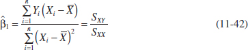
We note that the estimators of the intercept and slope in Equations 11-41 and 11-42 are identical to those given by the method of least squares in the case in which X was assumed to be a mathematical variable. That is, the regression model with Y and X jointly normally distributed is equivalent to the model with X considered as a mathematical variable. This follows because the random variables Y given X = x are independently and normally distributed with mean β0 + β1x and constant variance ![]() . These results will also hold for any joint distribution of Y and X such that the conditional distribution of Y given X is normal.
. These results will also hold for any joint distribution of Y and X such that the conditional distribution of Y given X is normal.
It is possible to draw inferences about the correlation coefficient ρ in this model. The estimator of ρ is the sample correlation coefficient

Note that
![]()
so the slope ![]() 1 is just the sample correlation coefficient R multiplied by a scale factor that is the square root of the “spread” of the Y values divided by the “spread” of the X values. Thus,
1 is just the sample correlation coefficient R multiplied by a scale factor that is the square root of the “spread” of the Y values divided by the “spread” of the X values. Thus, ![]() 1 and R are closely related, although they provide somewhat different information. The sample correlation coefficient R measures the linear association between Y and X, and
1 and R are closely related, although they provide somewhat different information. The sample correlation coefficient R measures the linear association between Y and X, and ![]() 1 measures the predicted change in the mean of Y for a unit change in X. In the case of a mathematical variable x, R has no meaning because the magnitude of R depends on the choice of spacing of x. We may also write, from Equation 11-44,
1 measures the predicted change in the mean of Y for a unit change in X. In the case of a mathematical variable x, R has no meaning because the magnitude of R depends on the choice of spacing of x. We may also write, from Equation 11-44,
![]()
which is just the coefficient of determination. That is, the coefficient of determination R2 is just the square of the correlation coefficient between Y and X.
It is often useful to test the hypotheses
![]()
The appropriate test statistic for these hypotheses is
Test Statistic for Zero Correlation

which has the t distribution with n − 2 degrees of freedom if H0: ρ = 0 is true. Therefore, we would reject the null hypothesis if |t0| > tα/2,n−2. This test is equivalent to the test of the hypothesis H0: β1 = 0 given in Section 11-5.1. This equivalence follows directly from Equation 11-46.
The test procedure for the hypotheses
![]()
where ρ0 ≠ 0 is somewhat more complicated. For moderately large samples (say, n ≥ 25), the statistic
![]()
is approximately normally distributed with mean and variance
![]()
respectively. Therefore, to test the hypothesis H0: ρ = ρ0, we may use the test statistic
and reject H0: ρ = ρ0 if the value of the test statistic in Equation 11-49 is such that |z0| > zα/2.
It is also possible to construct an approximate 100(1 − α) % confidence interval for ρ using the transformation in Equation 11-48. The approximate 100(1 − α) % confidence interval is
Confidence Interval for a Correlation Coefficient

where tanh u = (eu − e−u)/(eu + e−u).
Example 11-8 Wire Bond Pull Strength Chapter 1 (Section 1-3) describes an application of regression analysis in which an engineer at a semiconductor assembly plant is investigating the relationship between pull strength of a wire bond and two factors: wire length and die height. In this example, we will consider only one of the factors, the wire length. A random sample of 25 units is selected and tested, and the wire bond pull strength and wire length are observed for each unit. The data are shown in Table 1-2. We assume that pull strength and wire length are jointly normally distributed.
Figure 11-13 shows a scatter diagram of wire bond strength versus wire length. We have displayed box plots of each individual variable on the scatter diagram. There is evidence of a linear relationship between the two variables. Typical computer output for fitting a simple linear regression model to the data is on the next page.
Now Sxx = 698.56 and Sxy = 2027.7132, and the sample correlation coefficient is
![]()

FIGURE 11-13 Scatter plot of wire bond strength versus wire length, Example 11-8.
Note that r2 = (0.9818)2 = 0.9640 (which is reported in the computer output), or that approximately 96.40% of the variability in pull strength is explained by the linear relationship to wire length.
Now suppose that we wish to test the hypotheses

with α = 0.05. We can compute the t-statistic of Equation 11-46 as
![]()
This statistic is also reported in the computer output as a test of H0: β1 = 0. Because t0.025,23 = 2.069, we reject H0 and conclude that the correlation coefficient ρ ≠ 0.
Finally, we may construct an approximate 95% confidence interval on ρ from Equation 11-50. Because arctanh r = arctanh 0.9818 = 2.3452, Equation 11-50 becomes
![]()
which reduces to
![]()
Exercises FOR SECTION 11-8
![]() Problem available in WileyPLUS at instructor's discretion.
Problem available in WileyPLUS at instructor's discretion.
![]() Go Tutorial Tutoring problem available in WileyPLUS at instructor's discretion.
Go Tutorial Tutoring problem available in WileyPLUS at instructor's discretion.
11-76. ![]() Suppose that data are obtained from 20 pairs of (x, y) and the sample correlation coefficient is 0.8.
Suppose that data are obtained from 20 pairs of (x, y) and the sample correlation coefficient is 0.8.
(a) Test the hypothesis that H0: ρ = 0 against H1: ρ ≠ 0 with α = 0.05. Calculate the P-value.
(b) Test the hypothesis that H1: ρ = 0.5 against H1: ρ ≠ 0.5 with α = 0.05. Calculate the P-value.
(c) Construct a 95% two-sided confidence interval for the correlation coefficient. Explain how the questions in parts (a) and (b) could be answered with a confidence interval.
11-77. ![]() Suppose that data are obtained from 20 pairs of (x, y) and the sample correlation coefficient is 0.75.
Suppose that data are obtained from 20 pairs of (x, y) and the sample correlation coefficient is 0.75.
(a) Test the hypothesis that H0: ρ = 0 against H1: ρ > 0 with α = 0.05. Calculate the P-value.
(b) Test the hypothesis that H1: ρ = 0.5 against H1: ρ > 0.5 with α = 0.05. Calculate the P-value.
(c) Construct a 95% one-sided confidence interval for the correlation coefficient. Explain how the questions in parts (a) and (b) could be answered with a confidence interval.
11-78. A random sample of n = 25 observations was made on the time to failure of an electronic component and the temperature in the application environment in which the component was used.
(a) Given that r = 0.83, test the hypothesis that ρ = 0 using α = 0.05. What is the P-value for this test?
(b) Find a 95% confidence interval on ρ.
(c) Test the hypothesis H0: ρ = 0.8 versus H1: ρ ≠ 0.8, using α = 0.05. Find the P-value for this test.
11-79. A random sample of 50 observations was made on the diameter of spot welds and the corresponding weld shear strength.
(a) Given that r = 0.62, test the hypothesis that ρ = 0, using α = 0.01. What is the P-value for this test?
(b) Find a 99% confidence interval for ρ.
(c) Based on the confidence interval in part (b), can you conclude that ρ = 0.5 at the 0.01 level of significance?
![]()
11-80. The data in Table E11-6 gave x = the water content of snow on April 1 and y = the yield from April to July (in inches) on the Snake River watershed in Wyoming for 1919 to 1935. (The data were taken from an article in Research Notes, Vol. 61, 1950, Pacific Northwest Forest Range Experiment Station, Oregon.)
(a) Estimate the correlation between Y and X.
(b) Test the hypothesis that ρ = 0 using α = 0.05.
(c) Fit a simple linear regression model and test for significance of regression using α = 0.05. What conclusions can you draw? How is the test for significance of regression related to the test on ρ in part (b)?
(d) Analyze the residuals and comment on term list.
![]() 11-81.
11-81. ![]() Go Tutorial The final test and exam averages for 20 randomly selected students taking a course in engineering statistics and a course in operations research are in Table E11-7. Assume that the final averages are jointly normally distributed.
Go Tutorial The final test and exam averages for 20 randomly selected students taking a course in engineering statistics and a course in operations research are in Table E11-7. Assume that the final averages are jointly normally distributed.
(a) Find the regression line relating the statistics final average to the OR final average. Graph the data.
(b) Test for significance of regression using α = 0.05.
(c) Estimate the correlation coefficient.
(d) Test the hypothesis that ρ = 0, using α = 0.05.
(e) Test the hypothesis that ρ = 0.5, using α = 0.05.
(f) Construct a 95% confidence interval for the correlation coefficient.
![]()
11-82. The weight and systolic blood pressure of 26 randomly selected males in the age group 25 to 30 are shown in the Table E11-8. Assume that weight and blood pressure are jointly normally distributed.


(a) Find a regression line relating systolic blood pressure to weight.
(b) Test for significance of regression using α = 0.05.
(c) Estimate the correlation coefficient.
(d) Test the hypothesis that ρ = 0, using α = 0.05.
(e) Test the hypothesis that ρ = 0, using α = 0.05.
(f) Construct a 95% confidence interval for the correlation coefficient.
![]()
11-83. In an article in IEEE Transactions on Instrumentation and Measurement (2001, Vol. 50, pp. 986–990), researchers reported on a study of the effects of reducing current draw in a magnetic core by electronic means. They measured the current in a magnetic winding with and without the electronics in a paired experiment. Data for the case without electronics are provided in the Table E11-9.
(a) Graph the data and fit a regression line to predict current without electronics to supply voltage. Is there a significant regression at α = 0.05? What is the P-value?
(b) Estimate the correlation coefficient.
(c) Test the hypothesis that ρ = 0 against the alternative ρ ≠ 0 with α = 0.05. What is the P-value?
(d) Compute a 95% confidence interval for the correlation coefficient.
![]()
![]() TABLE • E11-8 Weight and Blood Pressure Data
TABLE • E11-8 Weight and Blood Pressure Data

![]() TABLE • E11-9 Voltage and Current Data
TABLE • E11-9 Voltage and Current Data

![]()
11-84. The monthly absolute estimate of global (land and ocean combined) temperature indexes (degrees C) in 2000 and 2001 (www.ncdc.noaa.gov/oa/climate/) are:
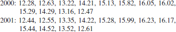
(a) Graph the data and fit a regression line to predict 2001 temperatures from those in 2000. Is there a significant regression at α = 0.05? What is the P-value?
(b) Estimate the correlation coefficient.
(c) Test the hypothesis that ρ = 0.9 against the alternative ρ ≠ 0.9 with α = 0.05. What is the P-value?
![]() TABLE • E11-10 Data for Correlation Exercise
TABLE • E11-10 Data for Correlation Exercise

(d) Compute a 95% confidence interval for the correlation coefficient.
11-85. ![]() Refer to the NFL quarterback ratings data in Exercise 11-5.
Refer to the NFL quarterback ratings data in Exercise 11-5.
(a) Estimate the correlation coefficient between the ratings and the average yards per attempt.
(b) Test the hypothesis H0: ρ = 0 versus H1: ρ ≠ 0 using α = 0.05. What is the P-value for this test?
(c) Construct a 95% confidence interval for ρ.
(d) Test the hypothesis H0: ρ = 0.7 versus H1: ρ ≠ 0.7 using α = 0.05. Find the P-value for this test.
11-86. ![]() Consider the (x, y) data in Table E11-10. Calculate the correlation coefficient. Graph the data and comment on the relationship between x and y. Explain why the correlation coefficient does not detect the relationship between x and y.
Consider the (x, y) data in Table E11-10. Calculate the correlation coefficient. Graph the data and comment on the relationship between x and y. Explain why the correlation coefficient does not detect the relationship between x and y.
11-9 Regression on Transformed Variables
We occasionally find that the straight-line regression model Y = β0 + β1x + ![]() is inappropriate because the true regression function is nonlinear. Sometimes nonlinearity is visually determined from the scatter diagram, and sometimes, because of prior experience or underlying theory, we know in advance that the model is nonlinear. Occasionally, a scatter diagram will exhibit an apparent nonlinear relationship between Y and x. In some of these situations, a nonlinear function can be expressed as a straight line by using a suitable transformation. Such nonlinear models are called intrinsically linear.
is inappropriate because the true regression function is nonlinear. Sometimes nonlinearity is visually determined from the scatter diagram, and sometimes, because of prior experience or underlying theory, we know in advance that the model is nonlinear. Occasionally, a scatter diagram will exhibit an apparent nonlinear relationship between Y and x. In some of these situations, a nonlinear function can be expressed as a straight line by using a suitable transformation. Such nonlinear models are called intrinsically linear.
As an example of a nonlinear model that is intrinsically linear, consider the exponential function
![]()
This function is intrinsically linear because it can be transformed to a straight line by a logarithmic transformation
![]()
This transformation requires that the transformed error terms ln ∈ are normally and independently distributed with mean 0 and variance σ2.
Another intrinsically linear function is
![]()
By using the reciprocal transformation z = 1 / x, the model is linearized to
![]()
Sometimes several transformations can be employed jointly to linearize a function. For example, consider the function
![]()
letting Y* = 1/Y, we have the linearized form
![]()
For examples of fitting these models, refer to Montgomery, Peck, and Vining (2012) or Myers (1990).
Transformations can be very useful in many situations in which the true relationship between the response Y and the regressor x is not well approximated by a straight line. The utility of a transformation is illustrated in the following example.
Example 11-9 Windmill Power A research engineer is investigating the use of a windmill to generate electricity and has collected data on the DC output from this windmill and the corresponding wind velocity. The data are plotted in Figure 11-14 and listed in Table 11-5.
Inspection of the scatter diagram indicates that the relationship between DC output Y and wind velocity (x) may be nonlinear. However, we initially fit a straight-line model to the data. The regression model is
![]()
The summary statistics for this model are R2 = 0.8745, MSE = ![]() 2 = 0.0557, and F0 = 160.26 (the P-value is <0.0001).
2 = 0.0557, and F0 = 160.26 (the P-value is <0.0001).
A plot of the residuals versus ![]() i is shown in Figure 11-15. This residual plot indicates model inadequacy and implies that the linear relationship has not captured all of the information in the wind speed variable. Note that the curvature that was apparent in the scatter diagram of Figure 11-14 is greatly amplified in the residual plots. Clearly, some other model form must be considered.
i is shown in Figure 11-15. This residual plot indicates model inadequacy and implies that the linear relationship has not captured all of the information in the wind speed variable. Note that the curvature that was apparent in the scatter diagram of Figure 11-14 is greatly amplified in the residual plots. Clearly, some other model form must be considered.
![]() TABLE • 11-5 Observed Values and Regressor Variable for Example 11-9
TABLE • 11-5 Observed Values and Regressor Variable for Example 11-9


FIGURE 11-14 Plot of DC output y versus wind velocity x for the windmill data.

FIGURE 11-15 Plot of residuals ei versus fitted values ![]() i for the windmill data.
i for the windmill data.
We might initially consider using a quadratic model such as
![]()
to account for the apparent curvature. However, the scatter diagram of Figure 11-14 suggests that as wind speed increases, DC output approaches an upper limit of approximately 2.5. This is also consistent with the theory of windmill operation. Because the quadratic model will eventually bend downward as wind speed increases, it would not be appropriate for these data. A more reasonable model for the windmill data that incorporates an upper asymptote would be
![]()
Figure 11-16 is a scatter diagram with the transformed variable x′ = 1/x. This plot appears linear, indicating that the reciprocal transformation is appropriate. The fitted regression model is
![]()
The summary statistics for this model are R2 = 0.9800, MSE = ![]() 2 = 0.0089, and F0 = 1128.43 (the P-value is <0.0001).
2 = 0.0089, and F0 = 1128.43 (the P-value is <0.0001).

FIGURE 11-16 Plot of DC output versus x′ = 1/x for the windmill data.

FIGURE 11-17 Plot of residuals versus fitted values ![]() i for the transformed model for the windmill data.
i for the transformed model for the windmill data.

FIGURE 11-18 Normal probability plot of the residuals for the transformed model for the windmill data.
A plot of the residuals from the transformed model versus ![]() is shown in Figure 11-17. This plot does not reveal any serious problem with inequality of variance. The normal probability plot, shown in Figure 11-18, gives a mild indication that the errors come from a distribution with heavier tails than the normal (notice the slight upward and downward curve at the extremes). This normal probability plot has the z-score value plotted on the horizontal axis. Because there is no strong signal of model inadequacy, we conclude that the transformed model is satisfactory.
is shown in Figure 11-17. This plot does not reveal any serious problem with inequality of variance. The normal probability plot, shown in Figure 11-18, gives a mild indication that the errors come from a distribution with heavier tails than the normal (notice the slight upward and downward curve at the extremes). This normal probability plot has the z-score value plotted on the horizontal axis. Because there is no strong signal of model inadequacy, we conclude that the transformed model is satisfactory.
Exercises FOR SECTION 11-9
![]() Problem available in WileyPLUS at instructor's discretion.
Problem available in WileyPLUS at instructor's discretion.
![]() Go Tutorial Tutoring problem available in WileyPLUS at instructor's discretion.
Go Tutorial Tutoring problem available in WileyPLUS at instructor's discretion.
11-87. Determine if the following models are intrinsically linear. If yes, determine the appropriate transformation to generate the linear model.
(a) ![]()
(b) ![]()
(c) ![]()
(d) ![]()
11-88. ![]() The vapor pressure of water at various temperatures is in Table E11-11:
The vapor pressure of water at various temperatures is in Table E11-11:
![]()
(a) Draw a scatter diagram of these data. What type of relationship seems appropriate in relating y to x?
(b) Fit a simple linear regression model to these data.
(c) Test for significance of regression using α = 0.05. What conclusions can you draw?
(d) Plot the residuals from the simple linear regression model versus ![]() i. What do you conclude about model adequacy?
i. What do you conclude about model adequacy?
(e) The Clausius–Clapeyron relationship states that ln (Pv) ∝ − ![]() where Pv is the vapor pressure of water. Repeat parts (a)–(d) using an appropriate transformation.
where Pv is the vapor pressure of water. Repeat parts (a)–(d) using an appropriate transformation.
![]() 11-89. An electric utility is interested in developing a model relating peak-hour demand (y in kilowatts) to total monthly energy usage during the month (x, in kilowatt hours). Data for 50 residential customers are shown in the Table E11-12.
11-89. An electric utility is interested in developing a model relating peak-hour demand (y in kilowatts) to total monthly energy usage during the month (x, in kilowatt hours). Data for 50 residential customers are shown in the Table E11-12.
(a) Draw a scatter diagram of y versus x.
(b) Fit the simple linear regression model.
![]() TABLE • E11-11 Vapor Pressure Data
TABLE • E11-11 Vapor Pressure Data

(c) Test for significance of regression using α = 0.05.
(d) Plot the residuals versus ![]() i and comment on the underlying regression assumptions. Specifically, does it seem that the equality of variance assumption is satisfied?
i and comment on the underlying regression assumptions. Specifically, does it seem that the equality of variance assumption is satisfied?
(e) Find a simple linear regression model using ![]() as the response. Does this transformation on y stabilize the inequality of variance problem noted in part (d)?
as the response. Does this transformation on y stabilize the inequality of variance problem noted in part (d)?
![]() TABLE • E11-12 Demand and Engery Usage Data
TABLE • E11-12 Demand and Engery Usage Data


11-10 Logistic Regression
Linear regression often works very well when the response variable is quantitative. We now consider the situation in which the response variable takes on only two possible values, 0 and 1. These could be arbitrary assignments resulting from observing a qualitative response. For example, the response could be the outcome of a functional electrical test on a semiconductor device for which the results are either a “success,” which means that the device works properly, or a “failure,” which could be due to a short, an open, or some other functional problem.
Suppose that the model has the form
![]()
and the response variable Yi takes on the values either 0 or 1. We will assume that the response variable Yi is a Bernoulli random variable with probability distribution as follows:

Now because E(![]() i) = 0, the expected value of the response variable is
i) = 0, the expected value of the response variable is
![]()
This implies that
![]()
This means that the expected response given by the response function E(Yi) = β0 + β1xi is just the probability that the response variable takes on the value 1.
There are some substantive problems with the regression model in Equation 11-51. First, note that if the response is binary, the error terms ![]() i can only take on two values, namely,
i can only take on two values, namely,
![]()
Consequently, the errors in this model cannot possibly be normal. Second, the error variance is not constant, because

Notice that this last expression is just
![]()
because E(Yi) = β0 + β1xi = πi. This indicates that the variance of the observations (which is the same as the variance of the errors because ![]() i = Yi − πi, and πi is a constant) is a function of the mean. Finally, there is a constraint on the response function because
i = Yi − πi, and πi is a constant) is a function of the mean. Finally, there is a constraint on the response function because
![]()
This restriction can cause serious problems with the choice of a linear response function as we have initially assumed in Equation 11-51. It would be possible to fit a model to the data for which the predicted values of the response lie outside the 0, 1 interval.
Generally, when the response variable is binary, there is considerable empirical evidence indicating that the shape of the response function should be nonlinear. A monotonically increasing (or decreasing) S-shaped (or reverse S-shaped) function, such as that shown in Figure 11-19, is usually employed. This function is called the logit response function, and has the form
![]()
or equivalently,
![]()

FIGURE 11-19 Examples of the logistic response function. (a) E(Y) = 1/(1 + e−6.0−1.0x). (b) E(Y) = 1/(1 + e− 6.0 + 1.0x).
In logistic regression, we assume that E(Y) is related to x by the logit function. It is easy to show that
![]()
The quantity in Equation 11-54 is called the odds. It has a straightforward interpretation: If the odds is 2 for a particular value of x, it means that a success is twice as likely as a failure at that value of the regressor x. Notice that the natural logarithm of the odds is a linear function of the regressor variable. Therefore, the slope β1 is the difference in the log odds that results from a one-unit increase in x. This means that the odds ratio equals eβ1 when x increases by one unit.
The parameters in this logistic regression model are usually estimated by the method of maximum likelihood. For details of the procedure, see Montgomery, Peck, and Vining (2012). Computer software will fit logistic regression models and provide useful information on the quality of the fit.
We will illustrate logistic regression using the data on launch temperature and O-ring failure for the 24 space shuttle launches prior to the Challenger disaster of January 1986. Six O-rings were used to seal field joints on the rocket motor assembly. The following table presents the launch temperatures. A “1” in the “O-Ring Failure” column indicates that at least one O-ring failure had occurred on that launch.

Figure 11-20 is a scatter plot of the data. Note that failures tend to occur at lower temperatures. The logistic regression model fit to these data from a computer software package is shown in the following boxed display. (Both Minitab and JMP have excellent capability to fit logistic regression models.)
The fitted logistic regression model is
![]()
The standard error of the slope ![]() 1 is se(
1 is se(![]() 1) = 0.08344. For large samples,
1) = 0.08344. For large samples, ![]() 1 has an approximate normal distribution, and so
1 has an approximate normal distribution, and so ![]() 1/se(
1/se(![]() 1) can be compared to the standard normal distribution to test H0: β1 = 0. Software performs this test. The P-value is 0.04, indicating that temperature has a significant effect on the probability of O-ring failure. The odds ratio is 0.84, so every 1 degree increase in temperature reduces the odds of failure by 0.84. Figure 11-21 shows the fitted logistic regression model. The sharp increase in the probability of O-ring failure is very evident in this graph. The actual temperature at the Challenger launch was 31°F. This is well outside the range of other launch temperatures, so our logistic regression model is not likely to provide highly accurate predictions at that temperature, but it is clear that a launch at 31°F is almost certainly going to result in O-ring failure.
1) can be compared to the standard normal distribution to test H0: β1 = 0. Software performs this test. The P-value is 0.04, indicating that temperature has a significant effect on the probability of O-ring failure. The odds ratio is 0.84, so every 1 degree increase in temperature reduces the odds of failure by 0.84. Figure 11-21 shows the fitted logistic regression model. The sharp increase in the probability of O-ring failure is very evident in this graph. The actual temperature at the Challenger launch was 31°F. This is well outside the range of other launch temperatures, so our logistic regression model is not likely to provide highly accurate predictions at that temperature, but it is clear that a launch at 31°F is almost certainly going to result in O-ring failure.

FIGURE 11-20 Scatter plot of O-ring failures versus launch temperature for 24 space shuttle flights.
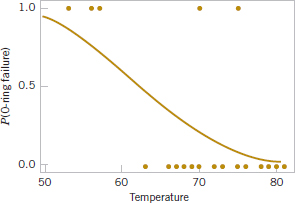
FIGURE 11-21 Probability of O-ring failure versus launch temperature (based on a logistic regression model).

It is interesting to note that all of these data were available prior to launch. However, engineers were unable to effectively analyze the data and use them to provide a convincing argument against launching Challenger to NASA managers. Yet a simple regression analysis of the data would have provided a strong quantitative basis for this argument. This is one of the more dramatic instances that points out why engineers and scientists need a strong background in basic statistical techniques.
Exercises FOR SECTION 11-10
![]() Problem available in WileyPLUS at instructor's discretion.
Problem available in WileyPLUS at instructor's discretion.
![]() Go Tutorial Tutoring problem available in WileyPLUS at instructor's discretion.
Go Tutorial Tutoring problem available in WileyPLUS at instructor's discretion.
![]() 11-90.
11-90. ![]() A study was conducted attempting to relate home ownership to family income. Twenty households were selected and family income was estimated along with information concerning home ownership (y = 1 indicates yes and y = 0 indicates no). The data are shown in Table E11-13.
A study was conducted attempting to relate home ownership to family income. Twenty households were selected and family income was estimated along with information concerning home ownership (y = 1 indicates yes and y = 0 indicates no). The data are shown in Table E11-13.
(a) Fit a logistic regression model to the response variable y. Use a simple linear regression model as the structure for the linear predictor.
(b) Is the logistic regression model in part (a) adequate?
(c) Provide an interpretation of the parameter β1 in this model.
![]()
11-91. ![]() The compressive strength of an alloy fastener used in aircraft construction is being studied. Ten loads were selected over the range 2500–4300 psi, and a number of fasteners were tested at those loads. The numbers of fasteners failing at each load were recorded. The complete test data are shown in Table E11-14.
The compressive strength of an alloy fastener used in aircraft construction is being studied. Ten loads were selected over the range 2500–4300 psi, and a number of fasteners were tested at those loads. The numbers of fasteners failing at each load were recorded. The complete test data are shown in Table E11-14.
(a) Fit a logistic regression model to the data. Use a simple linear regression model as the structure for the linear predictor.
(b) Is the logistic regression model in part (a) adequate?
![]() 11-92.
11-92. ![]() The market research department of a soft drink manufacturer is investigating the effectiveness of a price discount coupon on the purchase of a two-liter beverage product. A sample of 5500 customers was given coupons for varying price discounts between 5 and 25 cents. The response variable was the number of coupons in each price discount category redeemed after one month. The data follow in Table E11-15.
The market research department of a soft drink manufacturer is investigating the effectiveness of a price discount coupon on the purchase of a two-liter beverage product. A sample of 5500 customers was given coupons for varying price discounts between 5 and 25 cents. The response variable was the number of coupons in each price discount category redeemed after one month. The data follow in Table E11-15.
(a) Fit a logistic regression model to the data. Use a simple linear regression model as the structure for the linear predictor.
(b) Is the logistic regression model in part (a) adequate?
(c) Draw a graph of the data and the fitted logistic regression model.
(d) Expand the linear predictor to include a quadratic term. Is there any evidence that this quadratic term is required in the model?
![]()
![]() TABLE • E11-13 Home Ownership Data
TABLE • E11-13 Home Ownership Data

(e) Draw a graph of this new model on the same plot that you prepared in part (c). Does the expanded model visually provide a better fit to the data than the original model from part (a)?
![]() 11-93.
11-93. ![]() A study was performed to investigate new automobile purchases. A sample of 20 families was selected. Each family was surveyed to determine the age of their oldest vehicle and their total family income. A follow-up survey was conducted six months later to determine if they had actually purchased a new vehicle during that time period (y = 1 indicates yes and y = 0 indicates no). The data from this study are shown in the Table E11-16.
A study was performed to investigate new automobile purchases. A sample of 20 families was selected. Each family was surveyed to determine the age of their oldest vehicle and their total family income. A follow-up survey was conducted six months later to determine if they had actually purchased a new vehicle during that time period (y = 1 indicates yes and y = 0 indicates no). The data from this study are shown in the Table E11-16.
![]() TABLE • E11-14 Fastener Failure Data
TABLE • E11-14 Fastener Failure Data
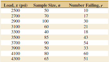
(a) Fit a logistic regression model to the data.
(b) Is the logistic regression model in part (a) adequate?
(c) Interpret the model coefficients β1 and β2.
(d) What is the estimated probability that a family with an income of $45,000 and a car that is five years old will purchase a new vehicle in the next six months?
![]() TABLE • E11-15 Coupon Redemption Data
TABLE • E11-15 Coupon Redemption Data

(e) Expand the linear predictor to include an interaction term. Is there any evidence that this term is required in the model?
11-94. ![]() The World Health Organization defines obesity in adults as having a body mass index (BMI) higher than 30. Of the 250 men in the study mentioned in Exercise 11-1, 23 are by this definition obese. How good is waist (size in inches) as a predictor of obesity? A logistic regression model was fit to the data:
The World Health Organization defines obesity in adults as having a body mass index (BMI) higher than 30. Of the 250 men in the study mentioned in Exercise 11-1, 23 are by this definition obese. How good is waist (size in inches) as a predictor of obesity? A logistic regression model was fit to the data:
![]()
where p is the probability of being classified as obese.
(a) Does the probability of being classified as obese increase or decrease as a function of waist size? Explain.
(b) What is the estimated probability of being classified as obese for a man with a waist size of 36 inches?
(c) What is the estimated probability of being classified as obese for a man with a waist size of 42 inches?
(d) What is the estimated probability of being classified as obese for a man with a waist size of 48 inches?
(e) Make a plot of the estimated probability of being classified as obese as a function of waist size.
![]() 11-95. Consider the propellant data is Exercise 11-13. Assume that strength less than 2100 psi is considered a failure. Relate propellant age to the probability of failure with a logistic regression model.
11-95. Consider the propellant data is Exercise 11-13. Assume that strength less than 2100 psi is considered a failure. Relate propellant age to the probability of failure with a logistic regression model.
(a) Does age have a significant effect on the probability of failure at a = 0.05?
(b) What is the estimated probability of failure when the storage time is 18 weeks?
(c) What is the effect of a one-week increase in storage on the odds of failure?
(d) Construct a plot of the estimated probability of failure as a function of age.
![]() TABLE • E11-16 Automobile Purchase Data
TABLE • E11-16 Automobile Purchase Data

Supplemental Exercises
![]() Problem available in WileyPLUS at instructor's discretion.
Problem available in WileyPLUS at instructor's discretion.
![]() Go Tutorial Tutoring problem available in WileyPLUS at instructor's discretion.
Go Tutorial Tutoring problem available in WileyPLUS at instructor's discretion.
11-96. Show that, for the simple linear regression model, the following statements are true:
(a) ![]()
(b) ![]()
(c) ![]()
![]() 11-97.
11-97. ![]() An article in the IEEE Transactions on Instrumentation and Measurement [“Direct, Fast, and Accurate Measurement of VT and K of MOS Transistor Using VT-Sift Circuit” (1991, Vol. 40, pp. 951–955)] described the use of a simple linear regression model to express drain current y (in milliamperes) as a function of ground-to-source voltage x (in volts). The data are as follows:
An article in the IEEE Transactions on Instrumentation and Measurement [“Direct, Fast, and Accurate Measurement of VT and K of MOS Transistor Using VT-Sift Circuit” (1991, Vol. 40, pp. 951–955)] described the use of a simple linear regression model to express drain current y (in milliamperes) as a function of ground-to-source voltage x (in volts). The data are as follows:

(a) Draw a scatter diagram of these data. Does a straight-line relationship seem plausible?
(b) Fit a simple linear regression model to these data.
(c) Test for significance of regression using α = 0.05. What is the P-value for this test?
(d) Find a 95% confidence interval estimate on the slope.
(e) Test the hypothesis H0: β0 = 0 versus H1: β0 ≠ 0 using α = 0.05. What conclusions can you draw?
![]()
11-98. ![]() The strength of paper used in the manufacture of cardboard boxes (y) is related to the percentage of hardwood concentration in the original pulp (x). Under controlled conditions, a pilot plant manufactures 16 samples, each from a different batch of pulp, and measures the tensile strength. The data follow:
The strength of paper used in the manufacture of cardboard boxes (y) is related to the percentage of hardwood concentration in the original pulp (x). Under controlled conditions, a pilot plant manufactures 16 samples, each from a different batch of pulp, and measures the tensile strength. The data follow:

(a) Fit a simple linear regression model to the data.
(b) Test for significance of regression using α = 0.05.
(c) Construct a 90% confidence interval on the slope β1.
(d) Construct a 90% confidence interval on the intercept β0.
(e) Construct a 95% confidence interval on the mean strength at x = 2.5.
(f) Analyze the residuals and comment on model adequacy.
![]() 11-99. Consider the following data. Suppose that the relationship between Y and x is hypothesized to be Y = (β0 + β1x +
11-99. Consider the following data. Suppose that the relationship between Y and x is hypothesized to be Y = (β0 + β1x + ![]() )−1. Fit an appropriate model to the data. Does the assumed model form seem reasonable?
)−1. Fit an appropriate model to the data. Does the assumed model form seem reasonable?

![]() 11-100.
11-100. ![]() The data in Table E11-17 adapted from Montgomery, Peck, and Vining (2012), present the number of certified mental defectives per 10,000 of estimated population in the United Kingdom (y) and the number of radio receiver licenses issued (x) by the BBC (in millions) for the years 1924
The data in Table E11-17 adapted from Montgomery, Peck, and Vining (2012), present the number of certified mental defectives per 10,000 of estimated population in the United Kingdom (y) and the number of radio receiver licenses issued (x) by the BBC (in millions) for the years 1924
![]() TABLE • E11-17 Data for Correlation Analysis
TABLE • E11-17 Data for Correlation Analysis

through 1937. Fit a regression model relating y and x. Comment on the model. Specifically, does the existence of a strong correlation imply a cause-and-effect relationship?
![]() 11-101. Consider the weight and blood pressure data in Exercise 11-82. Fit a no-intercept model to the data, and compare it to the model obtained in Exercise 11-82. Which model is superior?
11-101. Consider the weight and blood pressure data in Exercise 11-82. Fit a no-intercept model to the data, and compare it to the model obtained in Exercise 11-82. Which model is superior?
![]()
11-102. An article in Air and Waste [“Update on Ozone Trends in California's South Coast Air Basin” (1993, Vol. 43)] reported on a study of the ozone levels on the South Coast air basin of California for the years 1976–1991. The author believes that the number of days that the ozone level exceeds 0.20 parts per million depends on the seasonal meteorological index (the seasonal average 850 millibar temperature). The data are in Table E11-18:
(a) Construct a scatter diagram of the data.
(b) Fit a simple linear regression model to the data. Test for significance of regression.
(c) Find a 95% CI on the slope β1.
(d) Analyze the residuals and comment on model adequacy.
![]() 11-103. An article in the Journal of Applied Polymer Science (1995, Vol. 56, pp. 471–476) reported on a study of the effect of the mole ratio of sebacic acid on the intrinsic viscosity of copolyesters. The data follow:
11-103. An article in the Journal of Applied Polymer Science (1995, Vol. 56, pp. 471–476) reported on a study of the effect of the mole ratio of sebacic acid on the intrinsic viscosity of copolyesters. The data follow:
![]()
![]() TABLE • E11-18 Ozone Level Data
TABLE • E11-18 Ozone Level Data

(a) Construct a scatter diagram of the data.
(b) Fit a simple linear repression model.
(c) Test for significance of regression. Calculate R2 for the model.
(d) Analyze the residuals and comment on model adequacy.
![]()
11-104. Two different methods can be used for measuring the temperature of the solution in a Hall cell used in aluminum smelting, a thermocouple implanted in the cell and an indirect measurement produced from an IR device. The indirect method is preferable because the thermocouples are eventually destroyed by the solution. Consider the following 10 measurements:

(a) Construct a scatter diagram for these data, letting x = thermocouple measurement and y = IR measurement.
(b) Fit a simple linear regression model.
(c) Test for significance a regression and calculate R2. What conclusions can you draw?
(d) Is there evidence to support a claim that both devices produce equivalent temperature measurements? Formulate and test an appropriate hypothesis to support this claim.
(e) Analyze the residuals and comment on model adequacy.
![]()
11-105. The grams of solids removed from a material (y) is thought to be related to the drying time. Ten observations obtained from an experimental study follow:
![]()
(a) Construct a scatter diagram for these data.
(b) Fit a simple linear regression model.
(c) Test for significance of regression.
(d) Based on these data, what is your estimate of the mean grams of solids removed at 4.25 hours? Find a 95% confidence interval on the mean.
(e) Analyze the residuals and comment on model adequacy.
![]() 11-106.
11-106. ![]() Cesium atoms cooled by laser light could be used to build inexpensive atomic clocks. In a study reported in IEEE Transactions on Instrumentation and Measurement (2001, Vol. 50, pp. 1224–1228), the number of atoms cooled by lasers of various powers were counted. The data are in Table E11-19.
Cesium atoms cooled by laser light could be used to build inexpensive atomic clocks. In a study reported in IEEE Transactions on Instrumentation and Measurement (2001, Vol. 50, pp. 1224–1228), the number of atoms cooled by lasers of various powers were counted. The data are in Table E11-19.
![]() TABLE • E11-19 Number of Atoms
TABLE • E11-19 Number of Atoms

(a) Graph the data and fit a regression line to predict the number of atoms from laser power. Comment on the adequacy of a linear model.
(b) Is there a significant regression at α = 0.05? What is the P-value?
(c) Estimate the correlation coefficient.
(d) Test the hypothesis that ρ = 0 against the alternative ρ ≠ 0 with α = 0.05. What is the P-value?
(e) Compute a 95% confidence interval for the slope coefficient.
![]() 11-107. The data in Table E11-20 related diamond carats to purchase prices. It appeared in Singapore's Business Times, February 18, 2000.
11-107. The data in Table E11-20 related diamond carats to purchase prices. It appeared in Singapore's Business Times, February 18, 2000.
(a) Graph the data. What is the relation between carat and price? Is there an outlier?
(b) What would you say to the person who purchased the diamond that was an outlier?
(c) Fit two regression models, one with all the data and the other with unusual data omitted. Estimate the slope coefficient with a 95% confidence interval in both cases. Comment on any difference.
![]() 11-108.
11-108. ![]() Table E11-21 shows the population and the average count of wood storks sighted per sample period for South Carolina from 1991 to 2004. Fit a regression line with population as the response and the count of wood storks as the predictor. Such an analysis might be used to evaluate the relationship between storks and babies. Is regression significant at α = 0.05? What do you conclude about the role of regression analysis to establish a cause-and-effect relationship?
Table E11-21 shows the population and the average count of wood storks sighted per sample period for South Carolina from 1991 to 2004. Fit a regression line with population as the response and the count of wood storks as the predictor. Such an analysis might be used to evaluate the relationship between storks and babies. Is regression significant at α = 0.05? What do you conclude about the role of regression analysis to establish a cause-and-effect relationship?
![]() TABLE • E11-20 Diamond Price Data
TABLE • E11-20 Diamond Price Data

![]() TABLE • E11-21 Stork Population Data
TABLE • E11-21 Stork Population Data

11-109. Suppose that we have n pairs of observations (xi, yi) such that the sample correlation coefficient r is unity (approximately). Now let zi = ![]() and consider the sample correlation coefficient for the n-pairs of data (xi, zi). Will this sample correlation coefficient be approximately unity? Explain why or why not.
and consider the sample correlation coefficient for the n-pairs of data (xi, zi). Will this sample correlation coefficient be approximately unity? Explain why or why not.
11-110. Consider the simple linear regression model Y = β0 + β1x + ![]() , with E(
, with E(![]() ) = 0, V(
) = 0, V(![]() ) = σ2, and the errors
) = σ2, and the errors ![]() uncorrelated.
uncorrelated.
(a) Show that cov (![]() 0,
0, ![]() 1) = −
1) = −![]() σ2/Sxx.
σ2/Sxx.
(b) Show that cov (![]() ,
, ![]() 1) = 0.
1) = 0.
11-111. Consider the simple linear regression model Y = β0 + β1x + ![]() , with E(
, with E(![]() ) = 0, V(
) = 0, V(![]() ) = σ2, and the errors
) = σ2, and the errors ![]() uncorrelated.
uncorrelated.
(a) Show that E(![]() 2) = E(MSE) = σ2.
2) = E(MSE) = σ2.
(b) Show that E(MSR) = σ2 + ![]() Sxx.
Sxx.
11-112. Suppose that we have assumed the straight-line regression model
![]()
but the response is affected by a second variable x2 such that the true regression function is
![]()
Is the estimator of the slope in the simple linear regression model unbiased?
11-113. Suppose that we are fitting a line and we wish to make the variance of the regression coefficient ![]() 1 as small as possible. Where should the observations xi, i = 1, 2,..., n, be taken so as to minimize V(
1 as small as possible. Where should the observations xi, i = 1, 2,..., n, be taken so as to minimize V(![]() 1)? Discuss the practical implications of this allocation of the xi.
1)? Discuss the practical implications of this allocation of the xi.
11-114. Weighted Least Squares. Suppose that we are fitting the line Y = β0 + β1x + ![]() , but the variance of Y depends on the level of x; that is,
, but the variance of Y depends on the level of x; that is,
![]()
where the wi are constants, often called weights. Show that for an objective function in which each squared residual is multiplied by the reciprocal of the variance of the corresponding observation, the resulting weighted least squares normal equations are

Find the solution to these normal equations. The solutions are weighted least squares estimators of β0 and β1.
11-115. Consider a situation in which both Y and X are random variables. Let sx and sy be the sample standard deviations of the observed x's and y's, respectively. Show that an alternative expression for the fitted simple linear regression model ![]() =
= ![]() 0 +
0 + ![]() 1x is
1x is
![]()
11-116. Suppose that we are interested in fitting a simple linear regression model Y = β0 + β1x + ![]() where the intercept, β0, is known.
where the intercept, β0, is known.
(a) Find the least squares estimator of β1.
(b) What is the variance of the estimator of the slope in part (a)?
(c) Find an expression for a 100(1 − α)% confidence interval for the slope β1. Is this interval longer than the corresponding interval for the case in which both the intercept and slope are unknown? Justify your answer.
Important Terms and Concepts
Analysis of variance table
Coefficient of determination
Confidence interval on the intercept
Confidence interval on the slope
Confidence interval on the mean response
Correlation coefficient
Empirical model
Error sum of squares
Intrinsically linear model
Least squares
Logistic regression
Logit response function
Mean squares
Model adequacy checking
Normal probability plot of residuals
Odds ratio
Outlier
Prediction interval on a future observation
Regression coefficients
Regression line
Regression sum of squares
Regressor
Residuals
Residual plots
Response variable
Scatter diagram
Significance of regression
Simple linear regression model standard errors
Statistical tests on model parameters
Transformations