10	Flow Measurement

“Think three times, measure twice and cut once.”

—Anonymous

I.    SCOPE

In this chapter, we will illustrate and analyze some of the more common methods for measuring flow rate in conduits, including the pitot tube, venturi, nozzle, and orifice meters. This is by no means intended to be a comprehensive or exhaustive treatment, however, as there are a great many other devices in use for measuring flow rate, such as turbine, vane, Coriolis, ultrasonic, and magnetic flow meters, vortex meters, etc., just to name a few (see, e.g., Miller, 1996; Baker, 2009). The examples considered here demonstrate the application of the fundamental conservation principles to the analysis of several of the most common devices. Control valves are typically employed in conjunction with flow metering devices in order to control or regulate the flow rate in a piping system. This chapter is concerned with flow measurement, and the consideration of control valves is presented in Chapter 11.

There is one important caveat regarding meter installation. Most meters assume that the flow profile across the tube is symmetrical. This generally requires that the meter be installed at least 10 pipe diameters downstream and 5 diameters upstream of any flow disturbance elements, such as elbows, valves, bends, contractions/expansions, etc. If this is not possible, it is sometimes possible to install “straightening vanes” in the pipe downstream and/or upstream of the source of the disturbance to minimize this effect.

II.    PITOT TUBE

As previously discussed, the volumetric flow rate of a fluid through a conduit may be determined by integrating the local (“point”) velocity over the cross section of the conduit:

$Q={\displaystyle \underset{A}{\int }\text{v}}dA$

(10.1)

If the conduit cross section is circular, this becomes

$Q={\displaystyle \underset{0}{\overset{\pi R^2}{\int }}\text{v}\left(r\right)}d{\left(\pi r\right)}^2=2\pi {\displaystyle \underset{0}{\overset{R}{\int }}\text{v}\left(r\right)rdr}$

(10.2)

The pitot tube is a device for measuring v(r), the local velocity at a given position in the conduit, as illustrated in Figure 10.1. The measured values of the local point velocity are then used in Equation 10.2 to determine the volumetric flow rate. The meter includes a differential pressure measuring device (e.g., a manometer, transducer, or DP cell) that measures the pressure difference between the two tubes. One tube is attached to a hollow probe that can be positioned at any radial location in the conduit, and the other is attached to the wall of the conduit, in the same axial plane as the end of the probe. The local velocity of the streamline that impinges on the tip of the probe is v(r). The fluid element that impacts the open end of the probe must come to rest at that point, because there is no flow possible through the probe or the DP cell. This is known as the stagnation point. The Bernoulli equation can be applied to the fluid streamline that impacts the probe tip:

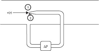
FIGURE 10.1 Pitot tube.

$\frac{P_2-P_1}{\rho }+\frac{1}{2}\left({\text{v}}_2^2-{\text{v}}_1^2\right)=0$

(10.3)

where

point 1 is in the free stream just upstream of the probe

point 2 is just inside the open end of the probe (the stagnation point)

Since the friction loss is negligible in the free stream from 1 to 2, and v₂ = 0 because the fluid in the probe is stagnant, Equation 10.3 can be solved for v₁ to give

${\text{v}}_1={\left(\frac{2\left(P_2-P_1\right)}{\rho }\right)}^{1/2}$

(10.4)

The measured pressure difference ΔP is the difference between the “stagnation” pressure in the velocity probe at the point where it connects to the DP cell and the “static” pressure at the corresponding point in the tube connected to the wall. Since there is no flow in the vertical direction, the difference in pressure between any two vertical elevations (at the same horizontal location) is strictly hydrostatic. Thus, the pressure difference measured at the DP cell is the same as that at the elevation of the probe, because the static head between point 1 and the pressure device is the same as that between point 2 and the pressure device, so that ΔP = P₂ − P₁.

We usually want to determine the total flow rate (Q) through the conduit, rather than the velocity at a point. This can be done by using Equation 10.1 or Equation 10.2 if the local velocity is measured at a sufficient number of radial points across the conduit to enable accurate evaluation of the integral. For example, the integral in Equation 10.2 could be evaluated by plotting the measured v(r) values as v(r) versus r², or as rv(r) versus r (in accordance with either the first or second form of Equation 10.2), and the area under the curve from r = 0 to r = R (the radius of the conduit) can be determined numerically.

The pitot tube is a relatively complex device and requires considerable effort and time to obtain an adequate number of velocity data points, especially close to the wall of the conduit, and to integrate these over the cross section to determine the total flow rate. On the other hand, the probe offers minimal resistance to the flow and hence is very efficient in that it results in negligible friction loss in the conduit. It is also the only practical means for determining the flow rate in very large conduits (such as smokestacks). There are standardized methods for applying this method to determine the total amount of material emitted through a stack, for example.

III.    VENTURI AND NOZZLE

There are other devices, however, that can be used to determine the flow rate from a single measurement. These are sometimes referred to as obstruction meters because the basic principle involves introducing an “obstruction” (e.g., a constriction) into the flow channel and measuring the pressure drop across the obstruction, which is then related to the flow rate.

Two such devices are the venturi meter and the nozzle, illustrated in Figure 10.2. In both cases, the fluid flows through a reduced area, which results in an increase in the velocity at that point. The corresponding change in pressure between point 1 upstream of the constriction and point 2 at the position of the minimum area (maximum velocity) is measured and is then related to the flow rate through the energy balance (the Bernoulli equation). The velocities are related by the continuity equation

${\rho }_1{V}_1{A}_1={\rho }_2{V}_2{A}_2$

(10.5)

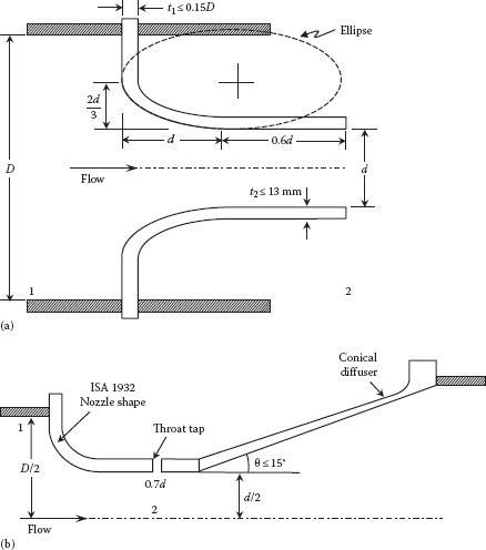
FIGURE 10.2 (a) ASME flow nozzle meter, (b) Venturi meter.

For a constant density fluid ρ₁ = ρ₂ which, with Equation 10.5, gives

$V_1=V_2\frac{A_2}{A_1}$

(10.6)

The Bernoulli equation relates the velocity change to the pressure change

$\frac{P_2-P_1}{\rho }+\frac{1}{2}\left(V_2^2-V_1^2\right)+e_f=0$

(10.7)

where plug flow has been assumed (so that the kinetic energy correction factor α is assumed to be equal to 1). Using Equation 10.6 to eliminate V₁ and neglecting the friction loss, Equation 10.7 can be solved for V₂:

$V_2={\left(\frac{-2\Delta P}{\rho \left(1-{\text{β}}^4\right)}\right)}^{1/2}$

(10.8)

where

ΔP = P₂ − P₁

β = d/D (where d is the minimum diameter at the throat of the venturi or nozzle and D is the pipe diameter)

To account for the inaccuracies introduced by assuming plug flow and neglecting friction, Equation 10.8 is written as

$V_2=C_d{\left(\frac{-2\Delta P}{\rho \left(1-{\text{β}}^4\right)}\right)}^{1/2}$

(10.9)

where C_d is the discharge coefficient, which is determined by calibration as a function of the Reynolds number for a given geometric design of the device. Typical values are shown in Figure 10.3, where

$N_{R{e}_D}=\frac{D{V}_{1\rho }}{\mu }\text{and}{N}_{R{e}_d}=\frac{d{V}_2\rho }{\mu }=\frac{N_{R{e}_D}}{\beta }$

Because the discharge coefficient accounts for the nonidealities in the system such as the friction loss, deviations from plug flow, etc., one would expect it to decrease with increasing Reynolds number, similar to the friction factor in pipe flow, although this is contrary to the trend in Figure 10.3. However, the discharge coefficient also accounts for the deviation from plug flow, which is greater at lower Reynolds numbers. In any event, the coefficient is not greatly different from 1.0, having a value of about 0.985 for (pipe) Reynolds numbers above about 2 × 10⁵, which indicates that these nonidealities are small, especially under turbulent flow conditions.

According to Miller (1996), for N_ReD > 4000, the discharge coefficient for the venturi, as well as for the nozzle and orifice, can be correlated as a function of N_ReD and β by the general equation

$C_d=C_{\infty }+\frac{b}{N_{R{e}_D}^n}$

(10.10)

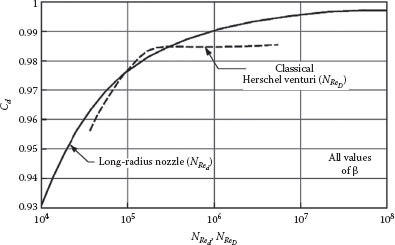
FIGURE 10.3 Venturi and nozzle discharge coefficient versus Reynolds number. (From White, F.M., Fluid Mechanics, 3rd edn., McGraw-Hill, New York, 1994.)

where the parameters C_∞, b, and n are given in Table 10.1 as a function of β. The range over which Equation 10.10 applies and its approximate accuracy are given in Table 10.2 (Miller, 1996). Because of the gradual expansion designed into the venturi meter, the pressure recovery is relatively large, so the net friction loss across the entire meter is a relatively small fraction of the measured (maximum) pressure drop, as indicated in Figure 10.4. However, because the flow area changes abruptly downstream of the orifice and nozzle, the expansion is uncontrolled, and considerable eddying occurs downstream. This dissipates more energy, resulting in a significantly higher net friction loss and lower pressure recovery, as also seen in Figure 10.4 and reflected by the relatively lower values of the discharge coefficient for the orifice and nozzle.

The foregoing equations assume that the device is horizontal, that is, that the pressure taps on the pipe are located in the same horizontal plane. If this is not the case, the equations can be easily modified to account for changes in elevation by replacing the pressure P at each point by the total potential Φ = P + ρgz.

The flow nozzle, illustrated in Figure 10.2, is similar to the venturi meter except that it does not include the diffuser (gradually expanding) section. In fact, one standard design for the venturi meter is basically a flow nozzle with an attached diffuser (see Figure 10.2). The equations that relate the flow rate and measured pressure drop in the nozzle are the same as for the venturi (e.g., Equation 10.9), and the nozzle (discharge) coefficient is also shown in Figure 10.3. It should be noted that the Reynolds number that is used for the venturi coefficient in Figure 10.3 is based on the pipe diameter (D), whereas the Reynolds number used for the nozzle coefficient is based on the nozzle diameter (d) (note that N_ReD = βN_Red). There are various “standard” designs for the nozzle, and the reader should consult the literature for details (e.g., Miller, 1996). The discharge coefficient for these nozzles can also be described by Equation 10.10, with the appropriate parameters given in Table 10.1.

IV.    ORIFICE METER

The simplest and most common device for measuring flow in a pipe is the orifice meter. This is an “obstruction” meter that consists of a plate with a hole in it that is inserted into the pipe, and the pressure drop across the plate is measured (as illustrated in Figure 10.5). The major difference between this device and the venturi and nozzle meters is the fact that the fluid stream leaving the orifice hole contracts to an area considerably smaller than that of the orifice hole. This is called the vena contracta, and it occurs because the fluid has considerable radial inward momentum as it converges into the orifice hole, which causes the flow to continue “inward” for a distance downstream of the orifice before it starts to expand to fill the pipe. If the pipe diameter is D, the orifice diameter is d, and the diameter of the vena contracta is d₂, the contraction ratio for the vena contracta is defined as C_c = A₂/A_o = (d₂/d)². For highly turbulent flow, C_c ≈ 0.6. Typical dimensions for a square-edged orifice are shown in Figure 10.6, and typical pressure tap locations are shown in Figure 10.7.

TABLE 10.1

Values for Discharge Coefficient Parameters^a in Equation 10.10

		Reynolds Number Term
Primary Device	Discharge Coefficient C∞ at Infinite Reynolds Number	Coefficient b	Exponent n
Venturi
Machined inlet	0.995	0	0
Rough cast inlet	0.984	0	0
Rough-welded	0.985	0	0
sheet-iron inlet
Universal venturi tubeb	0.9797	0	0
Lo-Loss tubec	1.05 – 0.471 β + 0.564β2 + 0.514β3	0	0
Nozzle
ASME long radius	0.9975	–6.53β0.5	0.5
ISA	0.9900 – 0.2262β4.1	1,708 – 8,936β + 19,779β4.7	1.15
Venturi nozzle (ISA inlet)	0.9858 – 0.195β4.5	0	0
Orifice
Corner taps	0.5959 + 0.0312β2.1 – 0.184β8	91.71β25	0.75
Flanged taps (D in in.)
D ≥ 2.3	0.5959 + 0.0312β2.1 − 0.184β8 + 0.09$\frac{{\beta }^4}{D\left(1-{\beta }^4\right)}-0.0337\frac{\beta }{D}$	91.71β2.5	0.75
2 ≤ D ≤ 2.3d	0.5959 + 0.0312β2.1 − 0.184β8 + 0.039$\frac{{\beta }^4}{1-{\beta }^4}-0.0337\frac{{\beta }^3}{D}$	91.71β2.5	0.75
Flanged taps (D* in mm)
D* ≥ 58.4	0.5959 + 0.0312β2.1 − 0.184β8$\frac{{\beta }^4}{D*\left(1-{\beta }^4\right)}-0.856\frac{{\beta }^3}{D*}$	91.71β2.5	0.75
50.8 ≤ D* ≤ 58.4	0.5959 + 0.0312β2.1 − 0.184β8 + 0.039$\frac{{\beta }^4}{1-{\beta }^4}-0.856\frac{{\beta }^3}{D^{*}}$	91.71β2.5	0.75
D and D/2 taps	0.5959 + 0.0312β2.1 − 0.184β8 + 0.039$\frac{{\beta }^4}{1-{\beta }^4}-0.0158{\beta }^3$	91.71β2.5	0.75
2½D and 8D tapsd	0.5959 + 0.461β2.1 – 0.48β8 + 0.039$\frac{{\beta }^4}{1-{\beta }^4}$	91.71β2.5	0.75

Source: Miller, R.W., Flow Measurement Engineering Handbook, 3rd edn., McGraw-Hill, New York, 1996.

a Detailed Reynolds number, line size, beta ratio, and other limitations are given in Table 10.2.

b From BIF CALC-440/441; the manufacturer should be consulted for exact coefficient information.

c Derived from the Badger meter, Inc. Lo-Loss tube coefficient curve; the manufacturer should be consulted for exact coefficient information.

d From Stolz (1978).

TABLE 10.2

Applicable Range and Accuracy of Equation 10.10, with Parameters from Table 10.1

Primary Device	Nominal Pipe Diameter D, in. (mm)	Ratio β	Pipe Reynolds Number, NReD, Range	Coefficient Accuracy (%)a
Venturi
Machined inlet	2–10 (50–250)	0.4–0.75	2 × 105 to 106	±1
Rough cast inlet	4–32(100–800)	0.3–0.75	2 × 105 to 106	±0.7
Rough-welded sheet-iron inlet	8–48 (100–1500)	0.4–0.7	2 × 105 to 106	±1.5
Universal venturi tubeb	≥3 (≥75)	0.2–0.75	>7.5 × 104	±0.5
Lo-Loss tubeb	3–120 (75–3000)	0.35–0.85	1.25 × 105 to 3.5 × 106	±1
Nozzle
ASME	2–16 (50–400)	0.25–0.75	104 to 107	±2.0
ISA	2–20 (50–500)	0.3–0.6	105 to 106	±0.8
		0.6–0.75	2 × 105 to 107	2β−0.4
Venturi nozzle	3–20 (75–500)	0.3–0.75	2 × 105 to 2 × 106	±1.2 ± 1.54β4
Orifice
Corner, flange, D and D/2	2–36 (50–900)	0.2–0.6	104 to 107	±0.6
		0.6−0.75	104 to 107	±β
		0.2–0.75	2 × 103 to 104	±0.6 ± β
2½D and 8D (pipe taps)	2–36 (50–900)	0.2–0.5	104 to107	±0.8
		0.51–0.7		±1.6
Eccentric Flange and vena contracta	4 (100)	0.3–0.75	104 to 106	±2
	6–14 (150–350)	0.3–0.75	104 to 106	±1.5
Segmental Flange and vena contracta	4–14 (150–350)	0.35–0.75	104 to 106	±2
Quadrant-edged Flanged and corner	1–4 (25–100)	0.25–0.6	250 to 6 × 104	±2 to ± 2.5
Conical entrance Corner		0.1–0.3	25 to 2 × 104	±2 to ± 2.5

Source: Miller, R.W., Flow Measurement Engineering Handbook, 3rd edn., McGraw-Hill, New York, 1996.

a ISO 5167 (1980) and ASME Fluid Meters (1971) show slightly different values for some devices.

b The manufacturer should be consulted for recommendation.

Note that Figure 10.6 shows the orifice hole to be beveled on the downstream side of the orifice plate. One purpose of this is to approximate the assumption that the orifice hole is in an “infinitely thin plate.” The downstream bevel also removes the downstream corner of the orifice hole to ensure that it does not interfere with the fluid stream leaving the orifice. It is not unusual to encounter orifice plates installed backwards, as seems logical by intuition. However, if this occurs, erratic or unreliable pressure readings may result.

The complete Bernoulli equation, as applied between point 1 upstream of the orifice where the diameter is D and point 2 at or near the vena contracta where the fluid stream diameter is d₂, is

${\displaystyle \underset{P_2}{\overset{P_1}{\int }}\frac{dP}{\rho }=\frac{1}{2}\left({\alpha }_2{V}_2^2-{\alpha }_1{V}_1^2\right)+\frac{K_f}{2}{V}_1^2}$

(10.11)

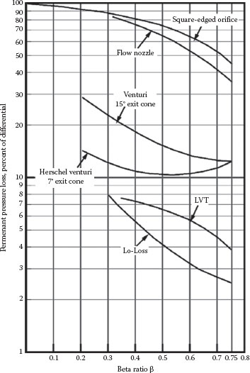
FIGURE 10.4 Unrecovered (friction) loss in various meters as a percentage of measured pressure drop versus β ratio. (From Cheremisinoff, N.P. and Cheremisinoff, P.N., Instrumentation for Process Flow Engineering, Technomic Publishing Company, Lancaster, PA, 1987.)

Just as for the other obstruction meters, when the continuity equation is used to eliminate the upstream velocity from Equation 10.11, the resulting expression can be solved for the mass flow rate through the orifice to give

$\dot{m}=\frac{C_0{A}_0{\rho }_2}{{\left(1-{\beta }^4\right)}^{1/2}}{\left[2{\displaystyle \underset{P_2}{\overset{P_1}{\int }}\frac{dP}{\rho }}\right]}^{1/2}$

(10.12)

where

β = d/D

C_o is the orifice discharge coefficient

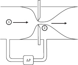
FIGURE 10.5 Orifice meter.

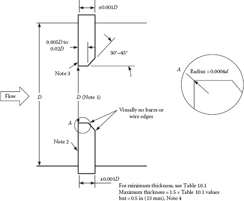
FIGURE 10.6 Concentric square-edged orifice specifications. Notes: (1) Mean of four diameters, no diameter >0.05% of mean diameter. (2) Maximum slope less than 1% from perpendicular: relative roughness <10⁻⁴ d over a circle not less than 1.5d. (3) Visually does not reflect a beam of light, finish with a fine radial cut from center outward. (4) ANSI/ASME MFC Draft 2 (July 1982), ASME, New York 1982. (From Miller, R.W., Flow Measurement Engineering Handbook, 3rd edn., McGraw-Hill, New York, 1996.)

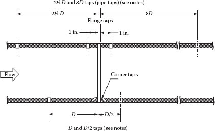
FIGURE 10.7 Orifice pressure tap locations. Notes: (1) 2½D and 8D pipe taps are not recommended in ISO 5167 or ASME Fluid Meters. (2) D and D/2 taps are now used in place of vena contracta taps. (From Miller, R.W., Flow Measurement Engineering Handbook, 3rd edn., McGraw-Hill, New York, 1996.)

$C_0=\frac{C_c}{\sqrt{{\alpha }_2}}{\left[\frac{1-{\beta }^4}{1-{\beta }^4{\left[C_c\left({\rho }_2/{\rho }_1\right)\right]}^2\left[\left({\alpha }_1-K_f\right)/{\alpha }_2\right]}\right]}^{1/2}$

(10.13)

where C_o is obviously a function of β, and the loss coefficient K_f (which depends on N_Re).

A.    INCOMPRESSIBLE FLOW

For incompressible flow, Equation 10.12 becomes

$\dot{m}=C_0{A}_0\sqrt{\frac{2\rho \Delta P}{\left(1-{\beta }^4\right)}}$

(10.14)

It is evident that the orifice coefficient incorporates the effects of both friction loss and velocity changes and must therefore depend upon the Reynolds number and the beta ratio. This is reflected in Figure 10.8, in which the orifice (discharge) coefficient is shown as a function of the orifice Reynolds number (N_Red) and β.

Actually, there are a variety of “standard” orifice plates and pressure tap designs (e.g., Miller, 1996). Figure 10.6 shows the ASME specifications for the most common concentric square-edged orifice. The various pressure tap locations, illustrated in Figure 10.7, are radius taps (one diameter upstream and D/2 downstream); flange taps (1 in. upstream and downstream); pipe taps (2½D upstream and 8D downstream); and corner taps. Radius taps, for which the location is scaled to the pipe diameter, are the most common. Corner taps and flange taps are the most convenient because they can be installed in the flange that holds the orifice plate and so do not require additional taps through the pipe wall. Pipe taps are less commonly used and essentially measure the total unrecovered pressure drop, or friction loss, through the orifice (which is usually quite a bit lower than the maximum pressure drop across the orifice plate). Vena contracta taps are sometimes specified, with the upstream tap one diameter from the plate and the downstream tap at the vena contracta location, although the latter varies with the Reynolds number and beta ratio and thus is not a fixed position.

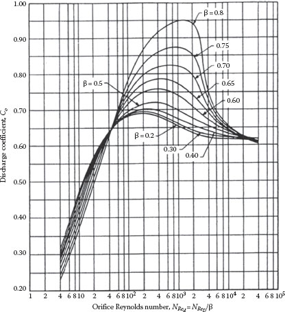
FIGURE 10.8 Orifice discharge coefficient for square-edged orifice and flange, corner, or radius taps. (From Miller, R.W., Flow Measurement Engineering Handbook, 3rd edn., McGraw-Hill, New York, 1996.)

Empirical (measured) values of the orifice coefficient are shown in Figure 10.8. This is valid to about 2%–5% (depending upon the Reynolds number) for all pressure tap locations except pipe and vena contracta taps. More accurate values can be calculated from Equation 10.10, with the parameter expressions given in Table 10.1 for the specific orifice and pressure tap arrangement.

B.    COMPRESSIBLE FLOW

Equation 10.14 applies to incompressible fluids such as liquids or gases under small pressure changes. For an ideal gas under adiabatic conditions (i.e., P/ρ^k = const), Equation 10.12 gives

$\dot{m}=C_o{A}_o{\left(\frac{P_1{\rho }_1}{1-\beta }\right)}^{1/2}{\left\{\frac{2k}{k-1}{\left(\frac{P_2}{P_1}\right)}^{2/k}\left[{\left(\frac{P_1}{P_2}\right)}^{\left(k-1\right)/k}-1\right]\right\}}^{1/2}$

(10.15)

It is more convenient to express this result in terms of the ratio of Equation 10.15 to the corresponding incompressible equation, Equation 10.14. The result is called the expansion factor Y:

$\dot{m}=C_o{A}_o{\left(\frac{P_1{\rho }_1}{1-\beta }\right)}^{1/2}{\left[2\left(1-\frac{P_2}{P_1}\right)\right]}^{1/2}$

(10.16)

where the density ρ₁ is evaluated at the upstream pressure (P₁). For convenience, the values of Y are shown as a function of ΔP/P₁ = (1 – P₂/P₁) and β for the square-edged orifice, nozzles, and venturi meters for values of k = c_p/c_v of 1.3 and 1.4 in Figure 10.9. The lines in Figure 10.9 for the orifice can be represented by the following equation for radius taps (Miller, 1996):

$Y=1-\frac{\Delta P}{k{P}_1}\left(0.41+0.35{\beta }^4\right)$

(10.17)

and for pipe taps by

$Y=1-\frac{\Delta P}{k{P}_1}\left[0.333+1.145\left({\beta }^2+0.7{\beta }^5+12{\beta }^{13}\right)\right]$

(10.18)

Note that there is no “button” at the ends of the lines for the orifice meter expansion factor, implying that the flow does not choke in an orifice. However, there is evidence that choked flow does occur downstream of an orifice at the vena contracta, but the lines in Figure 10.9 and Equations 10.17 and 10.18 do not apply beyond the range shown in Figure 10.9. A study by Kirk (2005) and Cunningham (1951) has indicated that the expansion factor for flange and radius taps follows Equation 10.17 for 1 > P₂/P₁ > 0.63 (or 0 < ΔP/P₁ < 0.37) and the following equation for 0.63 > P₂/P₁ > 0 (or 0.37 < ΔP/P₁ < 1.0):

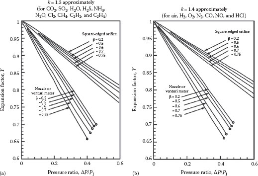
FIGURE 10.9 Expansion factor for orifice, nozzle, and venturi meter (a) k = 1.3, (b) k = 1.4. (From Crane Company, Flow of Fluids Through Valves, Fittings, and Pipe, Technical Manual 410, Crane Company, King of Prussia, PA, 1978.)

$Y=Y_{0.63}-\left(0.49+0.45{\beta }^4\right)\left(0.63-P_2/P_1\right)/k$

(10.19)

C.    FRICTION LOSS COEFFICIENT

The total friction loss in an orifice meter, after all pressure recovery has occurred, can be expressed in terms of a loss coefficient, K_f as follows. With reference to Figure 10.10, the total friction loss is (P₁ − P₃). By taking the system to be the fluid in the region from a point just upstream of the orifice plate (P₁) to a downstream position beyond the vena contracta where the stream has expanded to fill the pipe (P₃), the momentum balance becomes

${\displaystyle \sum _{onsystem}F=\dot{m}\left(V_3-V_1\right)=0=P_1{A}_o+P_2\left(A_1-A_o\right)-P_3{A}_1}$

(10.20)

The orifice equation (Equation 10.14) can be solved for the pressure drop (P₁ − P₂) to give

$P_1-P_2=\frac{\rho V_o^2}{2}\left(\frac{1-{\beta }^4}{C_o^2}\right)$

(10.21)

Eliminating P₂ from Equations 10.20 and 10.21 and solving for (P₁ − P₃) provides a definition for K_f based on the pipe velocity (V₁):

$P_1-P_3=\frac{\rho V_o^2\left(1-{\beta }^4\right)\left(1-{\beta }^2\right)}{2C_o^2}=\rho e_f=\frac{\rho V_1^2{K}_f}{2}$

(10.22)

Thus, the loss coefficient is

$K_f\approx \frac{\left(1-{\beta }^4\right)\left(1-{\beta }^2\right)}{C_o^2{\beta }^4}$

(10.23)

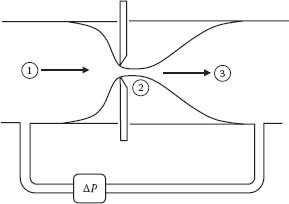
FIGURE 10.10 Friction loss in an orifice meter.

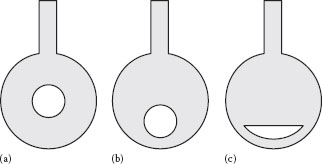
FIGURE 10.11 Other orifice geometries (a) Concentric, (b) eccentric, (c) segmental.

If the loss coefficient is based upon the velocity through the orifice (V_o) instead of the pipe velocity, the β⁴ term in the denominator of Equation 10.23 doesn’t appear:

$K_f\approx \frac{\left(1-{\beta }^4\right)\left(1-{\beta }^2\right)}{C_o^2}$

(10.24)

Equation 10.22 represents the net total (unrecovered) pressure drop due to friction in the orifice. This is expressed as a percentage of the maximum (orifice) pressure drop in Figure 10.4.

D.    OTHER GEOMETRIES

While the concentric orifice (hole in the center) is the most common design, eccentric and segmental orifice designs (Figure 10.11) are also used for the vapors and gases laden with small amount of contaminants (dust, condensed vapors, or other impurities heavier than the carrier such as dilute slurries, etc.). The designs shown in Figure 10.11 minimize the tendency for the deposition of impurities in front of the orifice plate. All such modifications necessitate the introduction of additional corrections to the formulae derived in this chapter. The discussion in this chapter is, however, restricted to concentric orifice plates.

V.    ORIFICE PROBLEMS

Three classes of problems involving orifices (or other obstruction meters) that the engineer might encounter are similar to the types of problems encountered in pipe flows. These are the “unknown pressure drop,” “unknown flow rate,” and “unknown orifice diameter” problems. Each involves relationships between the same five basic dimensionless variables: C_d, N_ReD, β, ΔP/P₁, and Y, where C_d represents the discharge coefficient for the meter. For incompressible liquids, this list reduces to four variables, because Y = 1 by definition. The basic orifice equation that relates these variables is

$\dot{m}=\frac{\pi D^2{\beta }^{2}Y{C}_d}{4}{\left(\frac{P_1{\rho }_1}{1-{\beta }^4}\right)}^{1/2}{\left[2\left(1-\frac{P_2}{P_1}\right)\right]}^{1/2}$

(10.25)

with

$N_{R{e}_D}=\frac{4\dot{m}}{\pi D\mu }\text{and}\beta =\frac{d}{D}$

(10.26)

and Y = fn(β, ΔP/P₁) (as given by Equation 10.17 or 10.18 or Figure 10.9), and C_d = fn(β, N_ReD) (as given by Equation 10.10 or Figure 10.8). The procedure for solving each of these problems is as follows.

A.    UNKNOWN PRESSURE DROP

In the case of an unknown pressure drop, we want to determine the pressure drop to be expected when a given fluid flows at a given rate through a given orifice meter:

Given: ṁ, μ, ρ₁, D, d (β = d/D), P₁ Find: ΔP

The procedure is as follows:

1.  Calculate N_ReD and β = d/D from Equation 10.26.

2.  Get C_d = C_o from Figure 10.8 or Equation 10.10.

3.  Assume Y = 1, and solve Equation 10.25 for (ΔP)₁:

${\left(\Delta P\right)}_1={\left(\frac{4\dot{m}}{\pi D^2{\beta }^2{C}_o}\right)}^2\left(\frac{1-{\beta }^4}{2{\rho }_1}\right)$

(10.27)

4.  Using (ΔP)_1/P₁ and β, get Y from Equation 10.17 or 10.18 or Figure 10.9.

5.  Calculate ΔP = (ΔP)₁/Y².

6.  Use the value of ΔP from step 5 in step 4, and repeat steps 4–6 until there is no change.

B.    UNKNOWN FLOW RATE

In the case of an unknown flow rate, the pressure drop across a given orifice is measured for a fluid with known properties, and the flow rate is to be determined.

Given: ΔP, P₁, D, d (β = d/D), μ, ρ₁ Find: ṁ

1.  Using ΔP/P₁ and β, get Y from Equation 10.17 or 10.18 or Figure 10.9.

2.  Assume C_o = 0.61.

3.  Calculate ṁ from Equation 10.25.

4.  Calculate N_ReD from Equation 10.26.

5.  Using N_ReD and β, get C_o from Figure 10.8 or Equation 10.10.

6.  If C_o ≠ 0.61, use the value from step 5 in step 3, and repeat steps 3–6 until there is no change.

C.    UNKNOWN DIAMETER

For design purposes, the proper size orifice (d or β) must be determined for a specified (maximum) flow rate of a given fluid in a given pipe with a ΔP device having a given (maximum) range.

Given: ΔP, P₁, μ, ρ, D, ṁ Find: d (i.e., β)

1.  Solve Equation 10.25 for β,

$\beta ={\left(\frac{X}{1+X}\right)}^{1/4}\text{where}X=\frac{8}{{\rho }_1\Delta P}{\left(\frac{\dot{m}}{\pi D^{2}Y{C}_o}\right)}^2$

(10.28)

2.  Assume that Y = 1 and C_o = 0.61.

3.  Calculate N_Red = N_ReD/ß, and get C_o from Figure 10.8 or Equation 10.10 and Y from Figure 10.9 or Equation 10.17 or 10.18.

4.  Use the results of step 3 in step 1, and repeat steps 1–4 until there is no change.

The required orifice diameter is d = βD.

VI.    NONINVASIVE TECHNIQUES

The discussion so far has been restricted to the so-called invasive methods (such as obstruction meters, venturi meter, etc.) of measuring local velocity and flow rate. The major disadvantage of this class of measuring method is that the flow is disturbed due to the insertion of the measuring sensor, like the pitot tube, orifice, or venturi device in the pipe. There are situations such as hostile temperature and pressure conditions, corrosive or abrasive nature of fluid, or issues with the contamination of the products such as in food, pharma, and health-care product sectors where it is not possible to use such devices. Further difficulties arise if the fluid is multiphase, such as slurries or suspensions of solids, gases, or immiscible liquids, or exhibits non-Newtonian flow characteristics (Fyrippi et al., 2004). Thus, over the years, a range of noninvasive techniques has been developed which can measure the flow rate of liquids or slurries or suspensions in pipes without disturbing the flow. Some of these are briefly described here, including their underlying principles.

A.    VORTEX-SHEDDING FLOW METER

When a fluid stream impinges on a bluff body (e.g., a cylinder) placed in its path, the boundary layers develop over the object and a wake (vortices) is formed in the rear of the bluff body. At a critical Reynolds number, these vortices begin to shed alternatively giving rise to the so-called von Karman vortex street (Figure 10.12). These vortices are shed at a well-defined frequency, which is proportional to the fluid velocity and which can be detected by oscillations of the bluff body. Vortex flow meters are quite versatile and can be used with clean gases and liquids, as described by Ginesi (1991) and Livelli (2013). However, this device cannot be used to measure low flow rates, as the vortex-shedding pattern is irregular under these conditions. The recommended minimum value of the pipe Reynolds number is of the order of ~30,000.

B.    MAGNETIC FLOW METER

This device measures volumetric flow rate directly and its operation hinges on well-known electromagnetic principles. Electrical current is induced in a conductor (the fluid) when it moves through a magnetic field. The voltage induced is directly proportional to the width of the conductor, the intensity of the magnetic fluid, and the velocity of the conductor. The process stream passes through the magnetic field induced by electromagnetic coils or permanent magnets built around a short length of pipe (called the metering section). Due to the magnetic field, the metering section must be made of nonmagnetic material or it must be lined with an electrically insulating material isolating it from the flowing liquid, which must be conducting. Commercial electromagnetic flow meters are now available for all sizes of pipes and have been found particularly suitable for metering flow rates in pharmaceutical and biological process engineering applications. Modern instruments can be used with conductivity levels as small as 0.5 μS/mm. These have also been shown to work reasonably well with non-Newtonian solutions and slurries (Heywood and Mehta, 1999; Fyrippi et al., 2004), with small loss in precision near the laminar-turbulent transition. This device is sensitive to the nature of the velocity profile in the pipe.

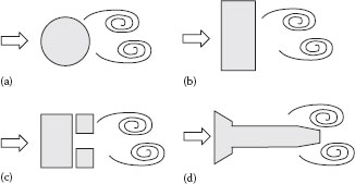
FIGURE 10.12 Schematics of vortex shedding sensors for a range of bluff body cross-sectional shapes.

C.    ULTRASONIC FLOW METER

Within this general class of flow meters, there are three types of devices based on different underlying principles, namely, time of flight method, frequency difference, and the Doppler effect. In the time of flight method, a high-frequency pressure wave is transmitted at an acute angle to the walls of the pipe which impinges on a receiver on the other side of the pipe (Figure 10.13). The elapsed time between transmission and reception depends on the velocity and velocity profile across the pipe, the speed of sound in the fluid, and the angle at which the wave is transmitted. In practice, a pair of transducers is used to exploit the fact that the velocity of an ultrasound pulse traveling against the flow direction is reduced, a and is increased when the pulse travels in the same direction. These meters are eminently suited for the flow measurements of water, clean liquids, liquefied gases, and natural gas.

The so-called frequency-difference ultrasonic flow meters employ two independent measuring paths, each having a transmitter–receiver pair (Figure 10.14). The arrival of a transmitted pulse at a receiver triggers the transmission of a further pulse thereby leading to the establishment of two distinct frequencies (in the upstream and downstream directions). The difference between these two frequencies is directly proportional to the velocity of the medium. The flow measurement is thus independent of the velocity of sound in the medium.

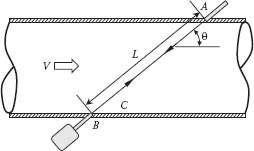
FIGURE 10.13 Ultrasonic flow meter. In the transit time meter two transducers (A and B) each act alternatively as the receiver and transmitter.

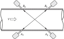
FIGURE 10.14 Frequency-difference ultrasonic flow meter.

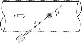
FIGURE 10.15 Doppler ultrasonic flow meter.

The Doppler ultrasonic flow meter may be used when small particles (solids, gas bubbles, droplets, or even strong eddies) are dispersed in the fluid. These are assumed to move essentially at the same velocity as the fluid medium to be metered. A continuous ultrasonic wave is transmitted at an acute angle to the wall of the pipe. The shift in frequency between the transmitted wave, which is scattered when incident on the particles, and that part of the wave which is reflected back to the receiver is measured (shown schematically in Figure 10.15). The shift in frequency between the transmitted and scattered waves is directly proportional to the flow velocity. However, the flow velocity must be much smaller than the velocity of sound in the fluid medium. This technique has gained wide spread acceptance for metering the flow of dilute slurries, dispersions, emulsions, etc.

D.    THE CORIOLIS FLOW METER

The flow meters described thus far measure velocity or volumetric flow rate, whereas the Coriolis flow meter measures mass flow rate. It comprises a sensor of one or more tubes which are made to vibrate at their resonant frequency by electromagnetic drivers, and the harmonic vibrations of the tubes impart an angular motion to the fluid as it passes through the tubes. This, in turn, exerts a Coriolis force on the tube walls. The magnitude of the Coriolis force is proportional to the product of density and velocity of the fluid. A secondary movement of the tubes occurs which is proportional to the mass flow rate which superimposes on the primary vibration, and the magnitude of the secondary oscillations is measured. More details can be found in the articles of Ginesi (1991), Reizner (2004), and Livelli (2013).

In addition to the bulk flow meters, highly sophisticated techniques like laser Doppler anemometer (LDA), magnetic resonance imaging (MRI), and particle image velocimetry (PIV) are also available which allow the measurement of point velocities as well as the fluctuating components in complex flow geometries. As of now, owing to their high costs and limited range of applicability in terms of fluid medium, etc., their use is limited to research only. Detailed descriptions together with their advantages and disadvantages are available in the literature (Adrian and Westerweel, 2010; Zhang, 2010; Smits and Lim, 2012).

SUMMARY

The significant points that should be retained from this chapter include the following:

•  The basic principles governing the operation of flow meters such as the pitot tube and obstruction meters such as the orifice, venturi, nozzle, etc.

•  Application of the orifice meter for incompressible and compressible flows

•  Determination of the unknown pressure drop, unknown flow rate, or unknown diameter for the orifice meter or other obstruction meter

•  Awareness of the large variety of other non-invasive flow meters such as vortex shedding, magnetic, Coriolis, ultrasonic, etc. meters and where to find information on them

PROBLEMS

FLOW MEASUREMENT

1.  An orifice meter with a hole of 1 in. diameter is inserted into a 1½ in. sch 40 line carrying SAE 10 lube oil at 70°F (SG = 0.93). A manometer using water as the manometer fluid is used to measure the orifice pressure drop reads 8 in. What is the flow rate of the oil in gallons per minute (gpm)?

2.  An orifice with a 3 in. diameter hole is mounted in a 4 in. diameter pipeline carrying water. A manometer containing an immiscible fluid with a specific gravity (SG) of 1.2 connected across the orifice reads 0.25 in. What is the flow rate in the pipe in gpm?

3.  An orifice with a 1 in. diameter hole is installed in a 2 in. sch 40 pipeline carrying SAE 10 lube oil at 100°F. The pipe section where the orifice is installed is vertical, with the flow being upward. Pipe taps that are 10.5 pipe diameters apart are used, which are connected to a manometer containing mercury to measure the pressure drop. If the manometer reading is 3 in., what is the flow rate of the oil in gpm?

4.  The flow rate in a 1.5 in. ID line can vary from 100 to 1000 bbl/day, and you must install an orifice meter to measure it. If you use a differential pressure (DP) cell with a range of 10 in. H₂O to measure the pressure drop across the orifice, what size orifice should you use? After this orifice is installed, you find that the DP cell reads 0.5 in. H₂O. What is the flow rate in barrels per day (bbl/day)? The fluid in the pipe is an oil with an SG = 0.89 and μ = 1 cP.

5.  A 4 in. sch 80 pipe carries water from a storage tank on top of a hill to a plant at the bottom of the hill. The pipe is inclined at an angle of 20° to the horizontal. An orifice meter with a diameter of 1 in. is inserted in the line, and a mercury manometer across the meter reads 2 in. What is the flow rate in gpm?

6.  You must size an orifice meter to measure the flow rate of gasoline (SG = 0.72) in a 10 in. ID pipeline at 60°F. The maximum flow rate expected is 1000 gpm, and the maximum pressure differential across the orifice is to be 10 in. of water. What size orifice should you use?

7.  A 2 in. sch 40 pipe carries SAE 10 lube oil at 100°F (SG = 0.928). The flow rate may be as high as 55 gpm, and you must select an orifice meter to measure the flow rate.

(a)  What size orifice should be used if the pressure difference is measured using a DP cell having a full-scale range of 100 in. H₂O?

(b)  Using this size orifice, what is the flow rate of oil in gpm when the DP cell reads 50 in. H₂O?

8.  A 2 in. sch 40 pipe carries a 35° API distillate at 50°F (SG = 0.85). The flow rate is measured by an orifice meter, which has a diameter of 1.5 in. The pressure drop across the orifice plate is measured by a water manometer connected to flange taps.

(a)  If the manometer reading is 1 in., what is the flow rate of the oil in gpm?

(b)  What would the diameter of the throat of a venturi meter be that would give the same manometer reading at this flow rate?

(c)  Determine the unrecovered pressure loss for both the orifice and the venturi in psi under these conditions.

9.  An orifice having a diameter of 1 in. is used to measure the flow rate of SAE 10 lube oil (SG = 0.928) in a 2 in. sch 40 pipe at 70°F. The pressure drop across the orifice is measured by a mercury (SG = 13.6) manometer, which reads 2 cm.

(a)  Calculate the volumetric flow rate of the oil in liters/second.

(b)  What is the temperature rise of the oil as it flows through the orifice in °F? (C_v = 0.5 Btu/(lbm °F)

(c)  How much power (in horsepower) is required to pump the oil through the orifice? (Note: this is the same as the rate of energy dissipated in the flow.)

10.  An orifice meter is used to measure the flow rate of CCl₄ in a 2 in. sch 40 pipe. The orifice diameter is 1.25 in., and a mercury (SG = 13.6) manometer attached to the pipe taps across the orifice reads 1/2 in. Calculate the volumetric flow rate of CCl₄ in ft³/s (SG of CCl₄ = 1.6). What is the permanent energy loss in the flow due to the presence of the orifice in ft lb_f/lb_m? Express this also as a total overall “unrecovered” pressure loss in psi.

11.  An orifice meter is installed in a 6 in. ID pipeline that is inclined upward at an angle of 10° from the horizontal. Benzene is flowing in the pipeline at the flow rate of 10 gpm. The orifice diameter is 3.5 in., and the orifice pressure taps are 9 in. apart.

(a)  What is the pressure drop between the pressure taps in psi?

(b)  What would be the reading of a water manometer connected to the pressure taps?

12.  You are to specify an orifice meter for measuring the flow rate of a 35° API distillate (SG = 0.85) flowing in a 2 in. sch 160 pipe at 70°F. The maximum flow rate expected is 2000 gph, and the available instrumentation for a differential pressure measurement has a limit of 2 psi. What size hole should the orifice plate have?

13.  You must select an orifice meter for measuring the flow rate of an organic liquid (SG = 0.8, μ = 15 cP) in a 4 in. sch 40 pipe. The maximum flow rate anticipated is 200 gpm, and the orifice pressure difference is to be measured with a mercury (SG = 13.6) manometer having a maximum reading range of 10 in. What size should the orifice be?

14.  An oil with an SG of 0.9 and viscosity of 30 cP is transported in a 12 in. sch. 20 pipeline at a maximum flow rate of 1000 gpm. What size orifice should be used to measure the oil flow rate if a DP cell with a full-scale range of 10 in. H₂O is used to measure the pressure drop across the orifice? What size venturi would you use in place of the orifice in the pipeline, everything else being the same?

15.  You want to use a venturi meter to measure the flow rate of water, up to 1000 gpm, through an 8 in. sch 40 pipeline. To measure the pressure drop in the venturi, you have a DP cell with a maximum range of 15 in. H₂O pressure difference. What size venturi (i.e., throat diameter) should you specify?

16.  Gasoline is pumped through a 2 in. sch 40 pipeline upward into an elevated storage tank at 60°F. An orifice meter is mounted in a vertical section of the line, which uses a DP cell with a maximum range of 10 in. H₂O to measure the pressure drop across the orifice at radius taps. If the maximum flow rate expected in the line is 10 gpm, what size orifice should you use? If a water manometer with a maximum reading of 10 in. is used instead of the DP cell, what would the required orifice diameter be?

17.  You have been asked by your boss to select a flow meter to measure the flow rate of gasoline (SG = 0.85) at 70°F in a 3 in. sch 40 pipeline. The maximum expected flow rate is 200 gpm, and you have a DP cell (which measures differential pressure) with a range of 0–10 in. H₂O available.

(a)  If you use a venturi meter, what should the diameter of the throat be?

(b)  If you use an orifice meter, what diameter orifice should you use?

(c)  For a venturi meter with a throat diameter of 2.5 in., what would the DP cell read (in inches of water) for a flow rate of 150 gpm

(d)  For an orifice meter with a diameter of 2.5 in., what would the DP cell read (in inches of water) for a flow rate of 150 gpm.

(e)  How much power (in hp) is consumed by friction loss in each of the meters under the conditions of (c) and (d)?

18.  A 2 in. sch 40 pipe is carrying water at a flow rate of 8 gpm. The flow rate is measured by means of an orifice with a 1.6 in. diameter hole. The pressure drop across the orifice is measured using a manometer containing an oil with an SG of 1.3.

(a)  What is the manometer reading in inches?

(b)  What is the power (in hp) consumed as a consequence of the friction loss due to the orifice plate in the fluid?

19.  The flow rate of CO₂ in a 6 in. ID pipeline is measured by an orifice meter with a diameter of 5 in. The pressure upstream of the orifice is 10 psig, and the pressure drop across the orifice is 30 in. H₂O. If the temperature is 80°F, what is the mass flow rate of CO₂?

20.  An orifice meter is installed in a vertical section of a piping system, in which SAE 10 lube oil is flowing upward (at 100°F). The pipe is 2 in. sch 40, and the orifice diameter is 1 in. The pressure drop across the orifice is measured by a manometer containing mercury as the manometer fluid. The pressure taps are pipe taps (2½ ID upstream and 8 ID downstream), and the manometer reading is 3 in. What is the flow rate of the oil in the pipe in gpm?

21.  You must install an orifice meter in a pipeline to measure the flow rate of 35.6° API crude oil at 80°F. The pipeline diameter is 18 in. sch 40, and the maximum expected flow rate is 300 gpm. If the pressure drop across the orifice is limited to 30 in. H₂O or less, what size orifice should be installed? What is the maximum permanent pressure loss that would be expected through this orifice in psi?

22.  You are to specify an orifice meter for measuring the flow rate of a 35° API distillate (SG = 0.85) flowing in a 2 in. sch 160 pipe at 70°F. The maximum flow rate expected is 2000 gph (gal/h), and the available instrumentation for the differential pressure measurement has a limit of 2 psi. What size orifice should be installed?

23.  A 6 in. sch 40 pipeline is designed to carry SAE 30 lube oil at 80°F (SG = 0.87) at a maximum velocity of 10 ft/s. You must install an orifice meter in the line to measure the oil flow rate. If the maximum pressure drop to be permitted across the orifice is 40 in. H₂O, what size orifice should be used? If a venturi meter is used instead of an orifice, everything else being the same, how large should the venturi throat be?

24.  An orifice meter with a diameter of 3 in. is mounted in a 4 in. sch 40 pipeline carrying an oil with a viscosity of 30 cP and an SG of 0.85. A mercury manometer attached to the orifice meter reads 1 in. If the pumping stations along the pipeline operate with a suction (inlet) pressure of 10 psig and a discharge (outlet) pressure of 160 psig, how far apart should the pump stations be, if the pipeline is horizontal?

25.  A 35° API oil at 50°F is transported in a 2 in. sch 40 pipeline. The oil flow rate is measured by an orifice meter that is 1.5 in. in diameter, using a water manometer.

(a)  If the manometer reading is 1 in., what is the oil flow rate (in gpm)?

(b)  If a venturi meter is used instead of the orifice meter, what should the diameter of the venturi throat be to give the same reading as the orifice meter at the same flow rate?

(c)  Determine the unrecovered pressure loss for both the orifice and venturi meters.

26.  A 6 in. sch 40 pipeline carries a petroleum fraction (viscosity 15 cP, SG 0.85) at a velocity of 7.5 ft/s, from a storage tank at 1 atm pressure to a plant site. The line contains 1500 ft of straight pipe, 25 90° flanged elbows, and four open globe valves. The oil level in the storage tank is 15 ft above ground, and the pipeline discharge is at a point 10 ft above ground, at a pressure of 10 psig.

(a)  What is the required flow capacity (in gpm) and the head (pressure) to be specified for the pump needed to move the oil?

(b)  If the pump is 85% efficient, what horsepower motor is required to drive it?

(c)  If a 4 in. diameter orifice is inserted in the line to measure the flow rate, what would the pressure drop reading across it be at the specified flow rate?

27.  Water drains by gravity out of the bottom of a large tank, through a horizontal 1 cm ID tube, 5 m long that has a venturi meter mounted in the middle of the tube. The level in the tank is 4 ft above the tube, and a single open vertical tube is attached to the throat of the venturi. What is the smallest diameter of the venturi throat for which no air will be sucked through the tube attached to the throat? What is the flow rate of the water under this condition?

28.  Natural gas (CH₄) is flowing in a 6 in. sch 40 pipeline at 50 psig and 80°F. A 3 in. diameter orifice is installed in the line, which reads a pressure drop of 20 in. H₂O. What is the gas flow rate, in lb_m/h and scfm?

29.  A solvent (SG = 0.9, μ = 0.8 cP) is transferred from a storage tank to a process unit through a 3 in. sch 40 pipeline that is 2000 ft long. The line contains 12 elbows, four globe valves, an orifice meter with a diameter of 2.85 in., and a pump having the characteristics shown in Figure 8.2 with a 7¼ in. impeller. The pressures in the storage tank and the process unit are both 1 atm, and the process unit is 60 ft higher than the storage tank. What is the pressure reading across the orifice meter in in. H₂O?

NOTATION

A	Cross-sectional area, [L2]
Cd	Discharge coefficient for a flow meter, [—]
Co	Orifice coefficient, [—]
D	Pipe diameter, [L]
d	Orifice, nozzle, or venturi throat diameter, [L]
F	Force, [F = ML/t2]
k	Isentropic coefficient, cp/cv for ideal gas, [—]
Kf	Loss coefficient, [—]
ṁ	Mass flow rate, [M/t]
NRe	Reynolds number, [—]
P	Pressure, [F/L2 = M/Lt2]
Q	Volumetric flow rate, [L3/t]
R	Radius, [L]
r	Radial position, [L]
SG	Specific gravity, [—]
V	Spatial average velocity, [L/t]
v	Local velocity, [L/t]
Y	Expansion factor, [—]

GREEK

α	Kinetic energy correction factor, [—]
β	dD, [—]
Δ()	()2 – ()1
ρ	Density, [M/L3]
v	Kinematic viscosity, [L2/t] also Specific volume, [ft3/lbm]

SUBSCRIPTS

1	Reference point 1
2	Reference point 2
d	Of orifice, nozzle, or venturi throat
D	Of pipe
o	Orifice
scfh	Standard cubic feet per hour
v	Venturi, viscosity correction, vapor pressure

REFERENCES

Adrian, R.J. and J. Westerweel, Particle Image Velocimetry, Cambridge University Press, New York, 2010.

Baker, R.C., Flow Measurement Handbook, Cambridge University Press, Cambridge, U.K., 2009.

Cheremisinoff, N.P. and P.N. Cheremisinoff, Instrumentation for Process Flow Engineering, Technomic Publishing Company, Lancaster, PA, 1987.

Crane Company, Flow of Fluids Through Valves, Fittings, and Pipes, Technical Manual 410, Crane Company, King of Prussia, PA, 1978.

Cunningham, R., Orifice meters with supercritical compressible flow, Trans. ASME, 73, 625–633, July 1951.

Fyrippi, I.O. and M.P. Escudier, Flowmetering of non-Newtonian liquids, Flow Meas. Instrum., 15, 131–138, 2004.

Ginesi, D., A raft of flowmeters on tap, Chem. Eng., 98, 147–155, May 1991.

Heywood, N.I. and K.B. Mehta, Performance evaluation of eight electromagnetic flow meters with fine sand slurries. Proceedings of the Hydrotransport 14, Maastricht, the Netherlands, 1999, pp. 413–431.

Kirk, D., Tech memo—Y factor.doc, Dennis Kirk Engineering, Mount Lawley, WA, 2005.

Livelli, G., Selecting flow meters to minimize energy costs, Chem. Eng. Prog., 109, 34–39, May 2013.

Miller, R.W., Flow Measurement Engineering Handbook, 3rd edn., McGraw-Hill, New York, 1996.

Reizner, J.R., Exposing Coriolis mass flowmeters’ dirty little secret, Chem. Eng. Prog., 100, 24–30, March 2004.

Smits, A.J. and T.T. Lim, Flow Visualization: Techniques and Examples, 2nd edn., Imperial College Press, London, U.K., 2012.

White, F.M., Fluid Mechanics, 3rd edn., McGraw-Hill, New York, 1994.

Zhang, Z., LDA Application Methods: Laser Doppler Anemometry for Fluid Dynamics, Springer, New York, 2010.