13	Fluid–Solid Separations by Free Settling

“Scientists study the world as it is, engineers create the world that never has been.”

—Theodore von Karman, 1881–1963, Mathematician

I.    FLUID–SOLID SEPARATIONS

The separation of suspended solids from a carrier fluid is a requirement in many engineering operations, e.g., the extensive listings of wide ranging applications and the equipment available in Besendorfer (1996), Chen (1997), Wakeman and Tarleton (2005) and Fernando Concha (2014). The most appropriate method for achieving this depends upon the specific properties of the system, the most important being the size and density of the solid particles and the solids concentration (e.g., the “solids loading”) of the feed stream. For example, for relatively dilute systems (e.g., ~10% or less) of relatively large particles (e.g., ~100 μm or more) of fairly dense solids, a gravity settling tank may be appropriate, whereas for more dilute systems of smaller and/or lighter particles, a centrifuge may be more appropriate. For very fine particles or where very high separation efficiency is required, a “barrier” system may be needed, such as a filter or membrane. For highly concentrated systems, a gravity thickener may be adequate or, for more stringent requirements, a filter may be needed (e.g., Wakeman and Tarleton, 2005; Chen, 1997; Coulson et al., 1991).

In this chapter, we will consider relatively dilute systems, for which the effects of particle–particle interactions are relatively unimportant (e.g., gravity and centrifugal separation). Situations in which particle–particle interactions are negligible are referred to as free settling, as opposed to hindered settling in which such interactions are important. Figure 13.1 shows the approximate regions of solids concentration and density corresponding to free or hindered settling conditions. In Chapter 14, we will consider systems that are controlled by hindered settling or interparticle interactions (e.g., filtration and sedimentation processes).

II.    GRAVITY SETTLING

Solid particles can be removed from a dilute suspension by passing the suspension through a vessel that is large enough such that the vertical component of the fluid velocity is lower than the terminal velocity of the particles and the residence time is sufficiently long to allow the particles to settle out. A typical gravity settler is illustrated in Figure 13.2. If the upward velocity of the liquid (Q/A) is less than the terminal velocity of the particles (V_t), the particles will settle at the bottom; otherwise, they will be carried out with the overflow. If Stokes flow is applicable (i.e., N_Re < 1), the diameter of the smallest particle that will settle out is

$d={\left(\frac{18\mu Q}{g\Delta \rho A}\right)}^{1/2}$

(13.1)

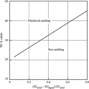
FIGURE 13.1 Approximate regions of hindered and free settling.

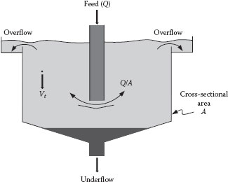
FIGURE 13.2 Schematic of a gravity settling tank.

If Stokes flow is not applicable (or even if it is), the Dallavalle equation in the form of Equation 12.17 can be used to determine the Reynolds number, and hence the diameter, of the smallest settling particle, that is,

$\frac{1}{\sqrt{N_{Re}}}={\left(0.00433+0.208\sqrt{\frac{C_D}{N_{Re}}}\right)}^{1/2}-0.0658$

(13.2)

where

$\frac{C_D}{N_{Re}}=\frac{4\mu \Delta \rho g}{3{\rho }^2{V}_t^3},d=\frac{N_{Re}\mu A}{Q\rho }$

(13.3)

Alternatively, it may be necessary to determine the maximum capacity (e.g., flow rate, Q) at which particles of a given size, d, will (or will not) settle out. This can also be obtained directly from the Dallavalle equation in the form of Equation 12.14, by solving for the unknown flow rate:

$Q=\left(\frac{\mu A}{d\rho }\right){\left[{\left(14.42+1.827\sqrt{N_{Ar}}\right)}^{1/2}-3.798\right]}^2$

(13.4)

where

$N_{Ar}=\frac{d^3\rho g\Delta \rho }{{\mu }^2}$

(13.5)

III.    CENTRIFUGAL SEPARATION

It is not strictly correct to classify centrifugal (and cyclone) separations as “free settling,” as the separation in these devices depends on a driving force established by an externally imposed centrifugal force. However, the principles involved in the analysis of these processes are all very similar, so it is reasonable to lump them together.

For very small particles or low-density solids, the terminal velocity may be too low to enable separation by gravity settling in a reasonably sized tank. However, the separation may be carried out in a centrifuge, which operates on the same principle as the gravity settler but employs the (radial) acceleration in a rotating system (e.g., ω²r) in place of the vertical gravitational acceleration as the driving force. Centrifuges can be designed to operate at very high rotating speeds, which may be equivalent to many “g’s” of acceleration, enhancing the separation.

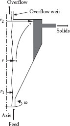
FIGURE 13.3 Schematic of a particle in a centrifuge.

A simplified schematic of a particle in a centrifuge is illustrated in Figure 13.3. It is assumed that any particle that impacts on the wall of the centrifuge (at r₂) before reaching the outlet will be trapped, and all others will not. (It might seem that any particle that impacts the outlet weir barrier would be trapped. However, the fluid circulates around this outlet corner setting up eddies that could sweep these particles out of the centrifuge). It is thus necessary to determine how far the particle will travel in the radial direction while in the centrifuge. To do this, we start with a radial momentum balance on the particle:

$F_{cf}-F_b-F_D=m_e\frac{d{V}_r}{dt}$

(13.6)

where

F_cf is the centrifugal force on the particle

F_b is the buoyant force (equal to the centrifugal force acting on the displaced fluid)

F_D is the drag force

m_e is the “effective” mass of the particle, which includes the solid particle and the “virtual mass” of the displaced fluid (i.e., half the actual mass of displaced fluid)

Equation 13.6 thus becomes

$\left({\rho }_s-\rho \right)\left(\frac{\text{π}{d}^3}{6}\right){\text{ω}}^{2}r-\rho V_r^2{C}_D\left(\frac{\text{π}{d}^3}{8}\right)=\left({\rho }_s+\frac{\rho }{2}\right)\left(\frac{\text{π}{d}^3}{6}\right)\frac{d{V}_r}{dt}$

(13.7)

When the particle reaches its terminal (radial) velocity, dV_r/dt = 0 and Equation 13.7 can be solved for V_rt (the radial terminal velocity):

$V_{rt}={\left(\frac{4\Delta \rho d{\text{ω}}^{2}r}{3\rho C_D}\right)}^{1/2}$

(13.8)

If N_Re < 1, Stokes’ law holds and C_D = 24/N_Re, in which case Equation 13.8 becomes

$V_{rt}=\frac{dr}{dt}=\frac{\Delta \rho d^2{\text{ω}}^{2}r}{18\mu }$

(13.9)

This shows that the terminal velocity is not a constant but increases with r, because the (centrifugal) driving force increases with r. Assuming that all of the fluid is rotating at the same speed as the centrifuge, integration of Equation 13.9 gives

$\text{ln}\left(\frac{r_2}{r_1}\right)=\frac{\Delta \rho d^2{\text{ω}}^2}{18\mu }t$

(13.10)

where t is the time required for the particle to travel a radial distance from r₁ to r₂. The time available for this to occur is the residence time of the particle in the centrifuge, that is,

$t=\frac{\tilde{V}}{Q}$

where $\tilde{V}$ is the volume of fluid in the centrifuge. If the region occupied by the fluid is cylindrical, then $\tilde{V}=\text{π}\left(r_2^2-r_1^2\right)L$. Combining the above two equations and solving for d gives the smallest particle that will travel from the surface of the fluid (r₁) to the wall (r₂) in time t

$d={\left(\frac{18\mu Q\text{ln}\left(r_2/r_1\right)}{\Delta \rho {\text{ω}}^2\tilde{V}}\right)}^{1/2}$

(13.11)

Rearranging Equation 13.11 to solve for Q gives

$Q=\frac{\Delta \rho d^2{\text{ω}}^2\tilde{V}}{18\mu \text{ln}\left(r_2/r_1\right)}=\left(\frac{\Delta \rho g{d}^2}{18\text{μ}}\right)\left(\frac{\tilde{V}{\text{ω}}^2}{g\text{ln}\left(r_2/r_1\right)}\right)$

(13.12)

which can also be written as

$Q=V_t\Sigma \text{where}\Sigma =\left(\frac{\tilde{V}{\text{ω}}^2}{g\text{ln}\left(r_2/r_1\right)}\right)$

(13.13)

where

V_t is the terminal velocity (in the radial direction) of the particle in a gravitational field

Σ is the cross-sectional area of the gravity settling tank that would be required to remove the same size particles as in the centrifuge

This driving force can be extremely large, if the centrifuge operates at a speed corresponding to “many g’s.”

This analysis is based on the assumption that Stokes’ law applies, that is, N_Re < 1. This is frequently a poor assumption, since many industrial centrifuges operate under conditions where N_Re > 1. If such is the case, an analytical solution to the problem is still possible using the Dallavalle equation for C_D, rearranged to solve for N_Re as follows:

$N_{Re}=\left(\frac{d\rho }{\mu }\right)\frac{dr}{dt}={\left[{\left(14.42+1.827\sqrt{N_{Ar}}\right)}^{1/2}-3.797\right]}^2$

(13.14)

where

$N_{Ar}=\frac{d^3\rho {\text{ω}}^{2}r\Delta \rho }{{\mu }^2}$

(13.15)

Equation 13.14 can be integrated from r₁ to r₂ and solved for t to give

$t=N_{12}\frac{\mu }{d^2{\text{ω}}^2\Delta \rho }$

(13.16)

where

$\begin{array}{ll}{N}_{12}\hfill & =0.599\left(N_{Re2}-N_{Re1}\right)+13.65\left(\sqrt{N_{Re2}}-\sqrt{N_{Re1}}\right)\hfill \\ \hfill & +17.29\text{ln}\left(\frac{N_{Re2}}{N_{Re1}}\right)+48.34\left(\frac{1}{\sqrt{N_{Re2}}}-\frac{1}{\sqrt{N_{Re1}}}\right)\hfill \end{array}$

(13.17)

The values of N_Re2 and N_Re1 are computed using Equation 13.14 and the values of N_Ar2 and N_Ar1 evaluated at r₁ and r₂, respectively. Since $t=\tilde{V}/Q$, Equation 13.16 can be rearranged to solve for Q:

$Q=\frac{\Delta \rho d^2{\text{ω}}^2\tilde{V}}{\mu N_{12}}=\frac{\Delta \rho d^2{\text{ω}}^2\tilde{V}}{18\mu \text{ln}\left(r_2/r_1\right)}\left[18\frac{\text{ln}\left(r_2/r_1\right)}{N_{12}}\right]$

(13.18)

where the term in the square brackets is a “correction factor” that can be applied to the Stokes flow solution to account for deviations from the Stokes flow assumption.

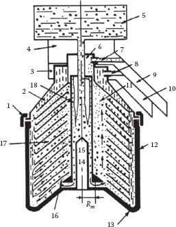
FIGURE 13.4 Schematic of a disk-bowl centrifuge: 1, Ring; 2, bowl; 3, 4, collectors for products; 5, feed tank; 6, tube; 7, 8, discharge nozzles; 9, 10, funnels for collectors; 11, through channels; 12, bowl; 13, bottom; 14, thick-walled tube; 15, hole for guide; 16, disk fixator; 17, disks; 18, central tube. (From Azbel, D.S. and Cheremisinoff, N.P., Fluid Mechanics and Unit Operations, Ann Arbor Science, Ann Arbor, MI, 1983.)

For separating very fine solids, emulsions, and immiscible liquids, a disk-bowl centrifuge is frequently used in which the settling occurs in the spaces between a stack of conical disks, as illustrated in Figure 13.4. The advantage of this arrangement is that the particles have a much smaller radial distance to travel before striking a wall and being trapped. The disadvantage is that the carrier fluid circulating between the disks has a higher velocity in the restricted spaces, which can retard the settling motion of the particles. Separation will occur only when V_rt > V_r, where V_rt is the radial terminal velocity of the particle and V_rf is the radial velocity component of the carrier fluid in the region where the fluid flow is in the inward radial direction.

A.    SEPARATION OF IMMISCIBLE LIQUIDS

The problem of separating immiscible liquids in a centrifuge can best be understood by first considering the static gravity separation, as illustrated in Figure 13.5, where the subscript 1 represents the lighter liquid and 2 represents the heavier liquid. In a continuous system, the static head of the heavier liquid in the overflow pipe must be balanced by the combined head of the lighter and heavier liquids in the separator, that is,

${\rho }_{2}zg={\rho }_2{z}_{2}g+{\rho }_1{z}_{1}g$

(13.19)

or

$z=z_2+z_1\frac{{\rho }_1}{{\rho }_2}$

(13.20)

In a centrifuge, the position of the overflow weir is similarly determined by the relative amounts of the heavier and lighter liquids and their densities, along with the size and speed of the centrifuge. The feed stream may consist of either the lighter liquid (1) dispersed in the heavier liquid (2) or vice versa. An illustration of the overflow weir positions is shown in Figure 13.6. Because there is no slip at the interface between the liquids, the axial velocity must be the same at that point for both fluids, that is,

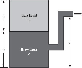
FIGURE 13.5 Gravity separation of immiscible liquids.

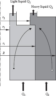
FIGURE 13.6 Centrifugal separation of immiscible liquids.

$\begin{array}{c}{V}_1=\frac{Q_1}{A_1}=\frac{Q_1}{\text{π}\left(r_i^2-r_1^2\right)}\\ V_2=\frac{Q_2}{A_2}=\frac{Q_2}{\text{π}\left(R^2-r_i^2\right)}\end{array}$

(13.21)

or

$\frac{Q_1}{Q_2}=\frac{r_i^2-r_1^2}{R^2-r_i^2}$

(13.22)

This provides a relation between the locations of the interface (r_i) and the inner weir (r₁) and the relative feed rates of the two liquids. Furthermore, the residence time for each of the two liquids in the centrifuge must be the same, that is,

$t=\frac{V_T}{Q_T}=\frac{\text{π}L\left(R^2-r_1^2\right)}{Q_1+Q_2}$

(13.23)

For drops of the lighter liquid (1) dispersed in the heavier liquid (2), assuming that Stokes flow applies, the time required for the drops to travel from the maximum radius (R) to the interface (r_i) is

$t=\frac{18{\mu }_2}{\Delta \rho d^2{\text{ω}}^2}\text{ln}\left(\frac{R}{r_i}\right)=\frac{\text{π}L\left(R^2-r_1^2\right)}{Q_1+Q_2}$

(13.24)

For drops of the heavier liquid (2) dispersed in the lighter liquid (1), the corresponding time required for the maximum radial travel from the surface (r₁) to the interface (r_i) is

$t=\frac{18{\mu }_1}{\Delta \rho d^2{\text{ω}}^2}\text{ln}\left(\frac{r_i}{r_1}\right)=\frac{\text{π}L\left(R^2-r_1^2\right)}{Q_1+Q_2}$

(13.25)

Equations 13.22 and 13.24 or Equation 13.25 determines the locations of the light liquid weir (r₁) and the interface (r_i) for given feed rates, centrifuge size, and operating conditions.

The proper location of the heavy liquid weir (r₂) can be determined by a balance of the radial pressure difference through the liquid layers, which is analogous to the gravity head balance in the gravity separator shown in Figure 13.5. The radial pressure gradient due to centrifugal force is

$\frac{dP}{dr}=\rho {\text{ω}}^{2}r\text{or}\Delta P=\frac{1}{2}\rho {\text{ω}}^2\Delta r^2$

(13.26)

Since both the heavy liquid surface at r₂ and the light liquid surface at r₁ are at atmospheric pressure, the sum of the pressure differences from r₁ to R to r₂ must be zero:

$\frac{1}{2}{\rho }_2{\text{ω}}^2\left(r_2^2-R^2\right)+\frac{1}{2}{\rho }_2{\text{ω}}^2\left(R^2-r_1^2\right)+\frac{1}{2}{\rho }_1{\text{ω}}^2\left(r_i^2-r_1^2\right)=0$

(13.27)

which can be rearranged to give

$\frac{{\rho }_2}{{\rho }_1}=\frac{r_i^2-r_1^2}{r_i^2-r_2^2}$

(13.28)

Solving for r₂:

$r_2^2=\frac{{\rho }_1}{{\rho }_2}\left[r_i^2\left(\frac{{\rho }_2}{{\rho }_1}-1\right)+r_1^2\right]$

(13.29)

Equations 13.22, 13.24, or 13.25 and 13.29 thus determine the three design parameters r_i, r₁, and r₂. These equations can be arranged in the following dimensionless form. From Equation 13.22:

${\left(\frac{r_1}{R}\right)}^2={\left(\frac{r_i}{R}\right)}^2\left(1+\frac{Q_1}{Q_2}\right)-\frac{Q_1}{Q_2}$

(13.30)

For drops of the light liquid in the heavy liquid, Equation 13.24 becomes

${\left(\frac{r_1}{R}\right)}^2=1-\frac{18{\mu }_2\left(Q_1+Q_2\right)}{\text{π}L{R}^2\Delta \rho d^2{\text{ω}}^2}\text{ln}\left(\frac{R}{r_i}\right)$

(13.31)

For drops of the heavy liquid in the light liquid, Equation 13.25 becomes

${\left(\frac{r_1}{R}\right)}^2=1-\frac{18{\mu }_1\left(Q_1+Q_2\right)}{\text{π}L{R}^2\Delta \rho d^2{\text{ω}}^2}\text{ln}\left[\left(\frac{r_i}{R}\right)\left(\frac{R}{r_1}\right)\right]$

(13.32)

Also, Equation 13.29 is equivalent to

${\left(\frac{r_2}{R}\right)}^2=\frac{{\rho }_1}{{\rho }_2}\left[\frac{r_i^2}{R^2}\left(\frac{{\rho }_2}{{\rho }_1}-1\right)+\frac{r_1^2}{R^2}\right]$

(13.33)

These three equations can be solved simultaneously (by iteration) for (r₁/R), (r₂/R), and (r_i/R). It is assumed that the size of the suspended drops is known, as are the density and viscosity of the liquids and the overall dimensions and speed of the centrifuge.

IV.    CYCLONE SEPARATIONS

A.    GENERAL CHARACTERISTICS

Centrifugal force can also be used to separate solid particles from fluids by inducing the fluid to undergo a rotating or spiraling flow pattern in a stationary vessel (e.g., a cyclone), which has no moving parts. Cyclones are widely used to remove small particles from gas streams (e.g., “aerocyclones”) and suspended solids from liquid streams (e.g., “hydrocyclones”).

A typical cyclone is illustrated in Figure 13.7 (this is sometimes referred to as a “reverse flow” cyclone). The suspension enters through a rectangular or circular duct tangential to the cylindrical separator, which usually has a conical bottom. The circulating flow generates a rotating vortex motion that imparts centrifugal force to the particles, which are thrown outward to the walls of the vessel where they fall by gravity to the conical bottom and are removed from the dusty gas. The carrier fluid spirals inward and downward to the cylindrical exit duct (also referred to as the “vortex finder”), where it travels back up and leaves the vessel at the top. The separation is not perfect, and some solid particles leave in the overflow as well as the underflow. The particle size for which 50% leaves in the overflow and 50% leaves in the underflow is called the cut size.

The diameter of hydrocyclones can range from 10 mm to 2.5 m, cut sizes from 2 to 250 μm, and flow rates (capacities) from 0.1 to 7200 m³/h. The pressure drop can range from 0.3 to 6 atm (Svarovsky, 1984). For aerocyclones, very little fluid leaves with the solids underflow, although for hydrocyclones the underflow solids content is typically 45%–50% by volume. Aerocyclones can separate particles as small as 2–5 μm.

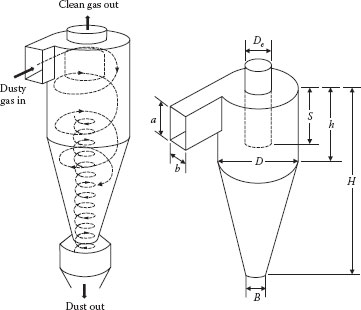
FIGURE 13.7 Typical reverse flow cyclone with geometric dimensions.

The advantages of the cyclone separator include the following (Svarovsky, 2000):

1.  Versatility—Virtually, any slurry or suspension can be concentrated, liquids degassed, or the solids classified by size, density, or shape.

2.  Simplicity and economy—They have no moving parts and require little maintenance.

3.  Small—Low residence times and relatively fast response.

4.  High shear forces—Can break up agglomerates, clusters of particles, friable solids etc.

The primary disadvantages are as follows:

1.  Inflexibility—A given design is not easily adapted to a range of conditions. Performance is strongly dependent upon flow rate and feed composition, and the turndown ratio (i.e., range of operation) is small.

2.  Limited separation performance—In terms of the sharpness of the cut, range of cut size, etc.

3.  Susceptibility to erosion for abrasive particles.

4.  High shear prevents utilization of flocculants to aid the separation, as can often be done in gravity settlers.

An increase in any one operating parameter generally increases all others, as well. For example, increasing the flow rate will increase both separation efficiency and pressure drop, and vice versa.

B.    AEROCYCLONES

1.  Velocity Distribution

Although the dominant velocity component in the cyclone is in the angular (tangential) direction, the swirling flow field includes significant velocity components in the radial and axial directions as well, which complicate the motion and makes a rigorous analysis impossible. This complex flow field also results in significant particle–particle collisions, which cause some particles of a given size to be carried out in both the overhead and underflow discharge, thus affecting the separation efficiency.

Cyclone analysis and design is not an exact science, and there are a variety of approaches to the analysis of cyclone performance. A critical review of the various methods for analyzing hydrocyclones has been given by Svarovsky (1996), and a review of different approaches to aerocyclone analysis has been given by Leith and Jones (1997). There are a number of different approaches to the analysis of aerocyclones, one of the most comprehensive being that of Bohnet et al. (1997). The presentation here follows that of Leith and Jones (1997), which outlines the basic principles and some of the practical “working relations.” The reader is referred to the additional references cited, especially the works of Bohnet (1983) and Bohnet et al. (1997), for more details on specific cyclone design.

The performance of a cyclone is dependent upon the geometry as described by the values of the various dimensionless “length ratios” (see Figure 13.7): a/D, b/D, D_e/D, S/D, h/D, H/D, and B/D. Typical values of these ratios for various “standard designs” are given in Table 13.1.

The complex three-dimensional flow pattern within the cyclone is dominated by the radial (V_r) and tangential (V_θ) velocity components. The vertical component is also significant but plays only an indirect role in the separation. The tangential velocity in the vortex varies with the distance from the axis in a complex manner, which can be described by the following equation:

$V_{\text{θ}}{r}^n=\text{constant}$

(13.34)

For a uniform angular velocity (ω = const., i.e., a “solid body rotation”) n = −1, whereas for a uniform tangential velocity (“plug flow”) n = 0, and for inviscid free vortex flow ω = c/r², that is, n = 1. Empirically, the exponent n has been found to vary typically between 0.5 and 0.9. The maximum value of V_θ occurs in the vicinity of the outlet or exit duct (vortex finder) at r = D_e/2. For aerocyclones, the exponent n has been correlated with the cyclone diameter by the following expression

$n=0.67D_m^{0.14}$

(13.35)

where D_m is the cyclone diameter in meters. The exponent also decreases as the temperature increases according to

$\frac{1-n}{1-n_1}={\left(\frac{T}{T_1}\right)}^{0.3}$

(13.36)

There is a “core” of rotating flow below the gas exit duct (vortex finder), in which the velocity decreases as the radius decreases and is nearly zero at the axis.

TABLE 13.1

Standard Designs for Reverse Flow Cyclones

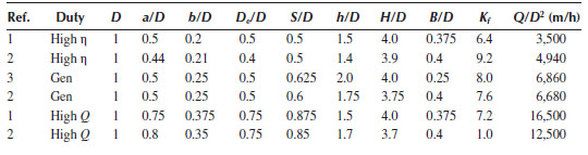
Source: Leith, D. and Jones, D.L., Cyclones, Chapter 15, in Handbook of Powder Science and Technology, 2nd edn., M.E. Fayed and L. Otten, (Eds.), Chapman & Hall, New York, 1997. 1. Stairmand (1951). 2. Swift (1969). 3. Lapple (1951).

2.  Pressure Drop

The pressure drops throughout the cyclone due to several factors: (1) gas expansion, (2) vortex formation, (3) friction loss, and (4) changes in kinetic energy. The total pressure drop can be expressed in terms of an equivalent loss coefficient, K_f:

$\Delta P=\frac{K_f{\rho }_G{V}_i^2}{2}$

(13.37)

where V_i is the gas inlet velocity, V_i = Q/ab. A variety of expressions have been developed for K_f, but one of the simplest that gives reasonable results is

$K_f=16\frac{ab}{D_e^2}$

(13.38)

This (and other) expression may be accurate to only about ±50% or so, and more reliable pressure drop information can only be obtained by experimental testing on a specific geometry. Typical values of K_f for the “standard” designs are also given in Table 13.1.

3.  Separation Efficiency

The efficiency of the cyclone (η) is defined as the fraction of particles of a given size, which is separated by the cyclone. The efficiency increases with the following trends:

1.  Increasing particle diameter (d) and density

2.  Increasing gas velocity

3.  Decreasing cyclone diameter

4.  Increasing cyclone length

5.  Venting some of the gas through the bottom solids exit

6.  Wetting the walls

A typical plot of efficiency versus particle diameter is shown in Figure 13.8. This is called a grade-efficiency curve. Although the efficiency varies with the particle size, a more easily determined characteristic is the “cut diameter” (d₅₀), which is that particle size collected with 50% efficiency.

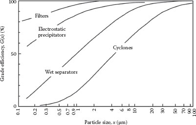
FIGURE 13.8 Typical cyclone grade-efficiency curve.

The particles are subject to centrifugal, inertial, and drag forces as they are carried in the spiraling flow, and it is assumed that the particles that strike the outer wall before the fluid reaches the vortex finder will be collected. It is assumed that the tangential velocity of the particle is the same as that of the fluid, that is, no slip (V_pθ = V_θ), but the radial velocity V_pr ≠ V_r, since the particles move radially toward the wall relative to the fluid. The centrifugal force acting on the particle is

$F_e=m_p{\text{ω}}^{2}r=\frac{\text{π}{d}^3{\rho }_s{V}_{\text{θ}}^2}{6r}$

(13.39)

Assuming Stokes flow, the drag force is

$F_d=3\text{π}\mu d\left(V_{pr}-V_r\right)$

(13.40)

Equation 13.34 provides a relation between the tangential velocity at any point and that at the wall:

$V_{\text{θ}}{r}^n=V_{\text{θ}w}{r}_w^n$

(13.41)

Although the velocity right at the wall is zero, the boundary layer at the wall is quite small, so this equation applies up to the boundary layer very near the wall. Setting the sum of the forces equal to the particle accelerating momentum and substituting V_pr = dr/dt and V_θ = V_θr(r_w/r)ⁿ gives the governing equation for the particle radial position as a function of time:

$\frac{d^{2}r}{d{t}^2}+\frac{18\mu }{d^2{\rho }_s}\frac{dr}{dt}-\left(\frac{V_{\text{θ}w}^2{r}_w^{2n}}{r^{\left(2n+1\right)}}+\frac{18\mu V_r}{d^2{\rho }_s}\right)=0$

(13.42)

There is no general solution to this nonlinear differential equation, and various analyses have been based upon specific approximations or simplifications of the equation. One approximation considers the time it takes for the particle to travel from the entrance point, r_i, to the wall, r_w = D/2, relative to the residence time of the fluid in the cyclone. By neglecting the acceleration term and the fluid radial velocity and assuming the velocity of the fluid at the entrance to be the same as the tangential velocity at the wall (V_i = V_θw), Equation 13.42 can be integrated to give the time required for the particle to travel from its initial position (r_i) to the wall (D/2). If this time is equal to or less than the residence time of the fluid in the cyclone, that particle will be trapped. The result thus gives the size of the theoretical smallest particle that will be trapped completely (in principle):

$d_{\mathit{100}}={\left[\frac{9\mu D^2{\left(1-2r_i/D\right)}^{\left(2n+2\right)}}{4\left(n+1\right)V_i^2{\rho }_{s}t}\right]}^{1/2}$

(13.43)

The residence time is related to the “number of turns” (N) that the fluid makes in the vortex, which can vary from 0.3 to 10, with an average value of 5. If the 50% “cut diameter” particle is assumed to enter at (D – b)/2, with a residence time of

$t=\frac{\text{π}DN}{V_i}\left(1-\frac{D_e}{2D}\right)$

(13.44)

and it is assumed that n = 0, then the cut diameter is

$d_{\mathit{50}}={\left(\frac{9\mu b}{2\text{π}{\rho }_s{V}_i{N}_i}\right)}^{1/2}$

(13.45)

Another approach is to consider the particle for which the drag force of the gas at the edge of the core (where the velocity is maximum) just balances the centrifugal force. This reduces Equation 13.42 to a “steady state,” with no net acceleration or velocity of the particle. The maximum velocity is given by Equation 13.41 applied at the edge of the core: $V_{\text{θ}w}^2{r}_w^{2n}=V_{\text{θ}}^2{r}_{core}^{2n}$. When this is introduced into Equation 13.42, the result is

$d_{\mathit{100}}={\left(\frac{9Q\mu }{\text{π}\left(H-S\right){\rho }_s{V}_{\max }^2}\right)}^{1/2}$

(13.46)

Although this predicts that all particles larger than this size will be trapped and all smaller particles will escape, the actual grade efficiency depends on the particle size because of the variation of the inward radial velocity of the gas.

Leith and Licht (1972) incorporated the effect of turbulent reentrainment of the solids in a solution of Equation 13.42 to derive the following expression for the grade efficiency:

$\text{η}=1-\exp \left[-2{\left(N_G{N}_{St}\right)}^{1/\left(2n+2\right)}\right]$

(13.47)

where

$N_{St}=\frac{d^2{\rho }_s{V}_i\left(n+1\right)}{18\mu D}$

(13.48)

is the Stokes’ number and N_G is a dimensionless geometric parameter, defined as

$\begin{array}{ll}{N}_G\hfill & =\frac{\text{π}{D}^2}{ab}\{2\left[1-{\left(\frac{D_e}{D}\right)}^2\right]\left(\frac{S}{D}-\frac{a}{2D}\right)+\frac{1}{3}\left(\frac{S+z_c-h}{D}\right)\hfill \\ \hfill & \times \left[1+\frac{d_c}{D}+{\left(\frac{d_c}{D}\right)}^2\right]+\frac{h}{D}-{\left(\frac{D_e}{D}\right)}^2\frac{z_c}{D}-\frac{S}{D}\}\hfill \end{array}$

(13.49)

where z_c is the core length, given by

$z_c=2.3D_e{\left(\frac{D^2}{ab}\right)}^{1/3}$

(13.50)

and d_c is the core diameter, given by

$d_c=D-\left(D-B\right)\left(\frac{S+z_c-h}{H-h}\right)$

(13.51)

Equation 13.47 implies that the efficiency increases as N_G and/or N_St increases.

These equations can serve as a guide for estimating performance but cannot be expected to provide precise prediction of the behavior. However, they can be used effectively to scale experimental results for similar designs of different sizes operating under various conditions. For example, two cyclones of a given design should have the same efficiency when the value of N_St is the same for both. That is, if a given cyclone has a known efficiency for particles of diameter d₁, a similar cyclone will have the same efficiency for particles of diameter d₂, where

$d_2=d_1{\left[\frac{Q_1}{Q_2}\left(\frac{{\rho }_{s1}}{{\rho }_{s2}}\right)\left(\frac{{\mu }_2}{{\mu }_1}\right)\left(\frac{D_2}{D_1}\right)\right]}^{1/2}$

(13.52)

Thus, the grade efficiency of a similar cyclone can be constructed from the grade efficiency of the known (tested) cyclone.

4.  Other Effects

Increasing the solids loading in the feed increases the collection efficiency and decreases the pressure drop. The reduction in pressure drop is attributed to the lowering of the tangential gas velocity due to the increased wall friction at high solids loading. The effect on pressure drop is given approximately by

${\left(\Delta P\right)}_c=\frac{{\left(\Delta P\right)}_o}{1+0.0086C_i^{1/2}}$

(13.53)

where C_i is the inlet solids loading in g/m³. On the other hand, the increased collection efficiency can be explained as follows: there is a critical load of particles that can be transported by the gas at a given velocity, and the amount of solids in excess of this load is deposited on the wall and captured by the cyclone, thereby increasing the overall efficiency. The effect of solids loading on overall collection efficiency is given by

$\frac{100-\text{η}}{100-{\text{η}}_1}={\left(\frac{C_{i1}}{C_i}\right)}^{0.182}$

(13.54)

If the velocity near the wall is too high, particles will bounce off the wall and become reentrained. The inlet velocity above which this effect occurs is given by the empirical correlation in SI units (Leith and Jones, 1997):

$V_{ic}=2400\left(\frac{\mu {\rho }_s}{{\rho }_G^2}\right)\left(\frac{D^{0.2}{\left(b/D\right)}^{1.2}}{1-b/D}\right)$

(13.55)

The cyclone efficiency increases with V_i up to about 1.25V_ic, after which reentrainment results in a decrease in efficiency.

C.    HYDROCYCLONES

A similar approach to the analysis of hydrocyclones has been presented by Svarovsky (2000), Besendorfer (1996), Salcudean et al., (2003), and others. They deduced that the system can be described in terms of three dimensionless groups, in addition to various dimensionless geometric parameters. These groups are the Stokes’ number:

$N_{St\mathit{50}}=\frac{V_{tr}}{V_i}=\frac{\Delta \rho d_{\mathit{50}}^{2}Q}{4\text{π}\mu D^3}$

(13.56)

the Euler number:

$N_{Eu}=\frac{\Delta P}{\rho V_i^2/2}=\frac{{\text{π}}^2\Delta P{D}^4}{8\rho Q^2}$

(13.57)

(which is equivalent to the loss coefficient, K_f), and the Reynolds number:

$N_{Re}=\frac{{DV}_{i\text{ρ}}}{\mu }=\frac{4Q\rho }{\text{π}D\mu }$

(13.58)

In each of these groups, the characteristic length is the cyclone diameter, D, and the characteristic velocity is V_i = 4Q/πD². Various empirical models for hydrocyclones indicate that the relationship between these groups can be represented by

$N_{St\mathit{50}}{N}_{Eu}=C$

(13.59)

and

$N_{Eu}=K_p{N}_{Re}^{n_p}$

(13.60)

The quantities C, K_p, and n_p are empirical constants, with the same values for a given family of geometrically similar cyclones. The value of C ranges from 0.06 to 0.33, the exponent n_p varies from 0 to 0.8, and K_p ranges from 2.6 to 6300. A summary of these parameters corresponding to some known hydrocyclone designs is given in Table 13.2 (Svarovsky, 1984). The references in this table are found in Svarovsky’s book, and the notation in the table is as follows: D_i = 2r_i = (4ab/π)^½ is the equivalent diameter of the inlet, D_o = D_e is the gas exit diameter, l = S is the length of the vortex finder, and L = H is the total length of the hydrocyclone. These equations can be used to predict the performance of a given cyclone as follows.

TABLE 13.2

Operational Parameters from Some Known Hydrocyclone Designs^a

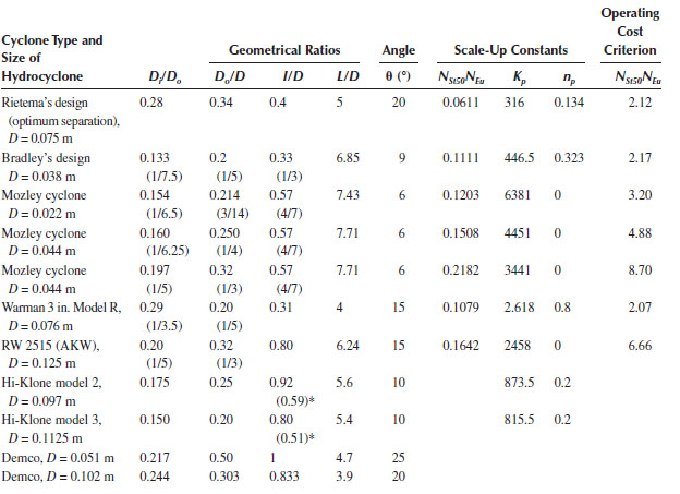
Source: Svarovsky, L., Hydrocyclones, Chapter 6, in Solid–Liquid Separation, L. Svarovsky, (Ed.), 4th edn., Butterworth Heinemann, Oxford, U.K., 2000.

^a Represents a modification; blank spaces in the table are where the figures are not known.

Equation 13.60 can be solved for the capacity, Q, to give

$Q^{2+n_p}=\frac{{\text{π}}^2\Delta P{D}^4}{8\rho K_p}{\left(\frac{\text{π}D\mu }{4\rho }\right)}^{n_p}$

(13.61)

and the cut size obtained from Equation 13.59:

$d_{\mathit{50}}^2=\frac{4\text{π}{N}_{St\mathit{50}}{N}_{Eu}{D}^3\mu }{K_{p}Q\Delta \rho }{\left(\frac{\text{π}D\mu }{4Q\rho }\right)}^{n_p}$

(13.62)

Actually, an extensive database reported by Medronho (Antunes and Medronho, 1992) indicates that the product N_St50N_Eu is not constant but depends on the underflow to feed ratio (R) and the feed volumetric concentration (C_v) and N_Eu also depends on C_v as well as N_Re.

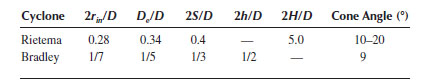
The Rietema and Bradley geometries are the two common families of geometrically similar designs, as defined by the geometric parameters in Table 13.3 (Antunes and Medronho, 1992). The Bradley hydrocyclone has a lower capacity than the Rietema geometry but is more efficient. For the Rietema cyclone geometry, the correlations are (Antunes and Medronho, 1992):

$N_{St\mathit{50}}{N}_{Eu}=0.0474{\left[\text{ln}\left(1/R\right)\right]}^{0.742}\exp \left(8.96C_{\text{v}}\right)$

(13.63)

and

$N_{Eu}=371.5N_{Re}^{0.116}\exp \left(-2.12C_{\text{v}}\right)$

(13.64)

where

$R=1218{\left(B/D\right)}^{4.75}{N}_{Eu}^{0.30}$

(13.65)

For the Bradley geometry, the corresponding correlations are (Antunes and Medronho, 1992)

$N_{Stk\mathit{50}}{N}_{Eu}=0.055{\left[\text{ln}\left(1/R\right)\right]}^{0.66}\exp \left(12C_{\text{v}}\right)$

(13.66)

and

$N_{Eu}=258N_{Re}^{0.37}$

(13.67)

where

$R=1.21\times {10}^6{\left(B/D\right)}^{2.63}{N}_{Eu}^{-1.12}$

(13.68)

TABLE 13.3

Families of Geometric Cyclones

These equations can be used to either predict the performance of a given cyclone or size a cyclone for given conditions. For example, if the definitions of N_Eu and N_Re from Equations 13.57 and 13.58 are substituted into Equation 13.67, the resulting expression for D is

$D=3.5\frac{{\rho }^{0.31}{Q}^{0.54}}{{\mu }^{0.085}{\left(\Delta P\right)}^{0.23}}$

(13.69)

which is dimensionally consistent.

SUMMARY

The main points to be retained from this chapter are

•  The distinction between “free” and “hindered” settling

•  Operation of the gravity settling tank

•  Analysis of centrifugal separators

•  Analysis of liquid–liquid separators

•  General principles and empirical correlations for separation efficiency of hydrocyclones and aerocyclones

PROBLEMS

FREE SETTLING FLUID–PARTICLE SEPARATIONS

1.    A slurry containing solid particles having a density of 2.4 g/cm³, ranging in diameter from 0.001 in. to 0.1 in., is fed to a settling tank 10 ft in diameter. Water is pumped into the tank at the bottom and overflows at the top, carrying some of the solid with it. If it is desired to separate out all particles of diameter 0.02 in. and smaller, what flow rate of the water in gpm is required?

2.    A handful of sand and gravel is dropped into a tank of water 5 ft deep. The time required for the solids to reach the bottom is measured and found to vary from 3 to 20 s. If the solid particles behave as equivalent spheres and have SG = 2.4, what is the range of equivalent particle diameters?

3.    It is desired to determine the size of pulverized coal particles by measuring the time it takes them to fall a given distance in a known fluid. It is found that the coal particles (SG = 1.35) take a time ranging from 5 s to 1000 min to fall 23 cm through a column of methanol (SG = 0.785, μ = 0.88 cP). What is the size range of the particles in terms of their equivalent spherical diameters? Assume the particles are falling at their terminal velocities at all times.

4.    A water slurry containing coal particles (SG = 1.35) is pumped into the bottom of a large tank (10 ft diameter, 6 ft high), at a rate of 500 gal/h, and overflows at the top. What is the largest coal particle that will be carried over in the overflow? If the flow rate is increased to 5000 gal/h, what size particles would you expect in the overflow? The slurry properties can be taken to be the same as for water.

5.    In order to determine the settling characteristics of a sediment, you drop a sample of the material into a column of water. You measure the time it takes for the solids to fall a distance of 2 ft and find that it ranges from 1 to 20 s. If the solid has a SG = 2.5, what is the range of particle sizes in the sediment, in terms of the diameters of equivalent spheres?

6.    You want to separate all the coal particles having a diameter of 100 μm or larger from a slurry. To do this, the slurry is pumped into the bottom of a large tank. It flows upward and overflows over the top of the tank, where it is collected in a trough. If the coal has SG = 1.4 and the total flow rate is 250 gpm, how big should the tank be?

7.    A gravity settling chamber consists of a horizontal rectangular duct 6 m long, 3.6 m wide, 3 m high. The duct is used to trap sulfuric acid mist droplets entrained in an air stream. The droplets settle out as the air passes through the duct and may be assumed to behave as rigid spheres. If the air stream has a flow rate of 6.5 m³/s, what is the diameter of the largest particle that will not be trapped by the duct? (For the Acid: ρ = 1.75 g/cm³, μ = 3 cP; For Air: ρ = 0.01 g/cm³, μ = 0.02 cP).

8.    Solid particles of diameter 0.1 mm and density 2 g/cm³ are to be separated from air in a horizontal settling chamber. If the air flow rate is 100 ft³/s and the maximum height of the chamber is 4 ft, what should the minimum length and width be for all of the particles to hit the bottom before exiting the chamber? (Air: ρ = 0.075 lb_m/ft³, μ = 0.018 cP).

9.    A settling tank contains solid particles that have a wide range of sizes. Water is pumped into the tank from the bottom and overflows on top at a rate of 10,000 gal/h. If the tank diameter is 3 ft, what separation of particle size is achieved (i.e., what size particles are carried out to the top of the tank, assuming the particles to be spherical)? Solid density = 150 lb_m/ft³.

10.  You want to use a viscous Newtonian fluid to transport small granite particles through a horizontal 1 in. ID 100 ft long pipeline. The granite particles have a diameter of 1.5 mm and SG = 4.0. The SG of the fluid can be assumed to be 0.95. The fluid should be pumped as fast as possible, to minimize settling of the particles in the pipe, but must be kept in laminar flow, so you design the system to operate at a pipe Reynolds number of 1000. The flow rate must be fast enough that the particles will not settle at a distance greater than 1/2 the ID of the pipe, from the entrance to the exit. What should the viscosity of the fluid be, and what should the flow rate be (in gpm) at which it is pumped through the pipe?

11.  An aqueous slurry containing particles with the size distribution shown in the following table is fed to a 20 ft diameter settling tank (see, e.g., McCabe et al. (1993) or Perry’s Handbook for the definition of mesh sizes):

Tyler Mesh Size	% of Total Solids in Feed
8/10	5.0
10/14	12.0
14/20	26.0
20/28	32.0
28/35	21.0
35/48	4.0

The feed enters near the center of the tank, and the liquid flows upward and overflows at the top of the tank. The solids loading of the feed is 0.5 lb_m of solids per gallon of slurry, and the feed rate is 50,000 gpm. What is the total solids concentration and particle size distribution in the overflow? The density of solids is 100 lb_m/ft³. Assume (1) the particles are spherical, (2) the particles in the tank are unhindered, and (3) the feed and overflow have the same properties as water.

12.  A water stream contacts a bed of particles, which have diameters ranging from 1 to 1000 μm and SG = 2.5. The water stream flows upward at a rate of 3 cm/s. What size particles will be carried out by the stream, and what size will be left behind?

13.  An aqueous slurry containing particles with SG = 4 and a range of sizes up to 300 μm flows upward through a small tube into a larger vertical chamber with a diameter of 10 cm. You want the liquid to carry all of the solids through the small tube, but you want only those particles with diameters less than 20 μm to be carried out to the top of the larger chamber. What should the flow rate of the slurry be (in gpm) and what size should the smaller tube be?

14.  A dilute aqueous CaCO₃ slurry is pumped into the bottom of a classifier, at a rate of 0.4 m³/s, and overflows at the top. The density of the solids is 2.71 g/cm³.

(a)  What should the diameter of the classifier be if the overflow is to contain no particles larger than 0.2 mm in diameter?

(b)  The same slurry as in (a) is sent to a centrifuge, which operates at 5000 rpm. The centrifuge diameter is 20 cm, its length is 30 cm, and the liquid layer thickness is 20% of the centrifuge radius. What is the maximum flow rate that the centrifuge can handle and achieve the same separation as the classifier?

15.  A centrifuge that is 40 cm ID and 30 cm long has an overflow weir that is 5 cm wide. The centrifuge operates at a speed of 3600 rpm.

(a)  What is the maximum capacity of the centrifuge (in gpm) for which particles with a diameter of 25 μm and SG = 1.4 can be separated from the suspension?

(b)  What would be the diameter of a settling tank that would do the same job?

(c)  If the centrifuge ID was 30 cm, how fast would it have to rotate to do the same job, everything else being equal?

16.  Solid particles with a diameter of 10 μm and SG = 2.5 are to be removed from an aqueous suspension in a centrifuge. The centrifuge inner radius is 1 ft, the outer radius is 2 ft, and length is 1 ft. If the required capacity of the centrifuge is 100 gpm, what should the operating speed (in rpm) be?

17.  A centrifuge is used to remove solid particles with a diameter of 5 μm and SG = 1.25 from a dilute aqueous stream. The centrifuge rotates at 1200 rpm and is 3 ft high, the radial distance to the liquid surface is 10 in., and the radial distance to the wall is 14 in.

(a)  Assuming that the particles must strike the centrifuge wall to be removed, what is the maximum capacity of this centrifuge, in gpm?

(b)  What is the diameter, in feet, of the gravity settling tank that would be required to do the same job?

18.  A dilute aqueous slurry containing solids with a diameter of 20 μm and SG = 1.5 is fed to a centrifuge rotating at 3000 rpm. The radius of the centrifuge is 18 in., its length is 24 in., and the overflow weir is 12 in. from the centerline.

(a)  If all of the solids are to be removed in the centrifuge, what is the maximum capacity that it can handle (in gpm)?

(b)  What is the diameter of the gravity settling tank that would be required for this separation, at the same flow rate?

19.  A centrifuge with a radius of 2 ft and a length of 1 ft has an overflow weir located 1 ft from the centerline. If particles with SG = 2.5 and diameters of 10 μm and less are to be removed from an aqueous suspension at a flow rate of 100 gpm, what should the operating speed of the centrifuge be (in rpm)?

20.  A centrifuge with a diameter of 20 in. operates at a speed of 1800 rpm. If there is a water layer 3 in. thick on the centrifuge wall, what is the pressure exerted on the wall?

21.  A vertical centrifuge, operating at 100 rpm, contains an aqueous suspension of solid particles with SG = 1.3 and radius of 1 mm. When the particles are 10 cm from the axis of rotation, determine the direction in which they are moving relative to a horizontal plane.

22.  You are required to design an aerocyclone to remove as much dust as possible from the exhaust coming from a rotary drier. The gas is air at 100°C, 1 atm, and a rate of 40,000 m³/h. The effluent from the cyclone will go to a scrubber for final cleanup. The maximum loading to the scrubber should be 10 g/m³, although 8 g/m³ or less is preferable. Measurements on the stack gas indicate that the solids loading from the drier is 50 g/m³. The pressure drop in the cyclone must be less than 2 kPa. Use the Stairmand standard design parameters from Table 13.1 as the basis for your design.

NOTATION

a	Cyclone inlet height, [L]
b	Cyclone inlet width, [L]
A	Cross-sectional area, [L2]
B	Cyclone bottom exit diameter, [L]
CD	Drag coefficient, [—]
Ci	Inlet solids loading, [M/L3]
d	Particle diameter, [L]
d50	Diameter of 50% cut particle, [L]
d100	Diameter of smallest trapped particle, [L]
D	Cyclone diameter, [L]
Dm	Cyclone diameter in meters, [L]
De	Cyclone top exit diameter, [L]
F	Force, [F = M L/t2]
Fc	Centrifugal force, [F = M L/t2]
g	Acceleration due to gravity, [L/t2]
H	Total cyclone height, [L]
h	Height of cyclone cylindrical section, [L]
Kf	Loss coefficient, [—]
me	Effective mass of moving particle, [M]
n	Exponent in Equation 13.34, [—]
N	Number of turns in vortex, [—]
NAr	Archimedes number, Equations 13.5 and 13.15, [—]
NEu	Euler number, Equation 13.57, [—]
NG	Dimensionless gravity number, Equation 13.49, [—]
NRe	Reynolds number, Equation 13.58, [—]
NSt	Stokes’ number, Equation 13.48, [—]
Nl2	Parameter defined by Equation 13.17, [—]
Q	Volumetric flow rate, [L3/t]
r	Radial position, [L]
S	Cyclone vortex finder height, [L]
T	Temperature, [T]
t	Time, [t]
V	Volume, [L3]
$\tilde{V}$	Volume of fluid in centrifuge, [L3]
Vr	Radial velocity of particle, [L/t]
Vrt	Radial terminal velocity of particle, [L/t]
Vt	Terminal velocity, [L/t]
V*t	Gravity settling velocity, [L/t]
Vθ	Tangential velocity in cyclone, [L/t]
z	Vertical distance measured upward, [L]

GREEK

η	Efficiency, [—]
Δ()	()2 – ()1
ρ	Density, [M/L3]
μ	Viscosity, [M/(L t)]
Σ	Equivalent gravity settling area for centrifuge, Equation 13.13, [L2]
ω	Angular velocity, [1/t]

SUBSCRIPTS

1,2	Reference points
c	Core
e	Exit
G	Gas
i	Inlet
o	Solids free
s	Solid
w	Wall
θ	Angular direction

REFERENCES

Antunes, M., and R.A. Medronho, Bradley cyclones: Design and performance analysis, in Hydrocyclones, Analysis and Applications, L. Svarovsky and M.T. Thew, (Eds.), Kluwer Academic Publishers, Dordrecht, The Netherlands, 1992.

Azbel, D.S. and N.P. Cheremisinoff, Fluid Mechanics and Unit Operations, Ann Arbor Science, Ann Arbor, MI, 1983.

Besendorfer, C., Exert the force of hydrocyclones, Chem. Eng., 103(9), 108–114, 1996.

Bohnet, M., Design methods for aerocyclones and hydrocyclones, Chapter 32, in Handbook of Fluids in Motion, N.P Cheremisinoff and R. Gupta, (Eds.), Ann Arbor Science, Ann Arbor, MI, 1983.

Bohnet, M., O. Gottschalk. and M. Morweiser, Modern design of aerocyclones, Adv. Particle Tech., 8(2), 137–161, 1997.

Chen, W., Solid-liquid separation, Chem. Eng., 104(2), 66–72, 1997.

Coulson, J.M., J.F. Richardson, J.R. Blackhurst, and J.H. Harker, Chemical Engineering, Vol. 2, 4th Ed., Pergamon Press, Oxford, U.K., 1991.

Fernando Concha, A., Solid-Liquid Separation in the Mining Industry, Springer, New York, 2014.

Lapple, C.E., Processes use many collection types, Chem. Eng., 58(5), 144–151, 1951.

Leith, D. and D.L. Jones, Cyclones, Chapter 15, in Handbook of Powder Science and Technology, 2nd edn., M.E. Fayed and L. Otten, (Eds.), Chapman & Hall, New York, 1997.

Leith, D. and W. Licht, The collection efficiency of cyclone type particle collectors - a new theoretical approach, AIChE Sym. Ser., 68, 196–206, 1972.

McCabe, W.L., J.C. Smith, and P. Harriott, Unit Operations of Chemical Engineering, McGraw-Hill, New York, 1993.

Salcudean, M., I. Gartshore, and E.C. Statie, Test hydrocyclones before they are built, Chem. Eng., 110(4), 66–71, 2003.

Starimand, C.J., Design and performance of cyclone separators, Trans. Inst. Chem. Engrs., 29, 356–372, 1951.

Svarovsky, L., Hydrocyclones, Technomic Publishing Co., Lancaster, PA, 1984.

Svarovsky, L., A critical review of hydrocyclone models, in Hydrocyclones ‘96, D. Claxton, L. Svarovsky, and M., Thew, (Eds.), Mechanical Engineering Publications Ltd., London, U.K., 1996.

Svarovsky, L., Hydrocyclones, Chapter 6, in Solid-Liquid Separation, L. Svarovsky, (Ed.), 4th edn., Butterworths, Oxford, U.K., 2000.

Swift, P., Dust controls in industry, Steam Heating Engr., 38, 453–456, 1969.

Wakeman, R.J. and E.S. Tarleton, Solid-Liquid Separation, Elsevier, London, U.K., 2005.