
“Engineering is learning how to make a decision with insufficient information.”
—Anonymous
The understanding of, and ability to predict, the flow behavior of fluids is fundamental to all aspects of the chemical engineering profession. Such behavior includes the relationship between the (driving) forces and the flow rates of various classes of fluids, and the characteristics of the equipment used to contain/handle/process these fluids. A wide variety of fluids with different properties may be encountered by the chemical engineer in the industrial applications that may be of concern in various chemical or petroleum process industries, biological or food and pharmaceutical industries, polymer and materials processing industries, etc. These properties range from common simple incompressible (Newtonian) liquids, that is, fluids such as water, oils, various petroleum fractions, etc., to complex nonlinear (non-Newtonian) fluids such as pastes, emulsions, foams, suspensions, high-molecular-weight polymeric fluids, biological fluids (e.g., blood), etc. as well as compressible (gaseous) fluids such as air, N2, CO2, etc. This book is concerned with the fundamental principles that govern the flow behavior of each of these types of fluids, as well as the resulting basic relationships needed to predict their behavior (relations between flow rates, pressures, forces on solid boundaries, etc.) and the corresponding analysis of a wide variety of equipment and practical situations commonly found in various industries. These principles are also applicable to such situations as the flow of blood in vessels, transport of sludge and silt in rivers and streams, pneumatic conveying of particles, the trajectory of a pitched baseball, etc.
The fundamental principles that apply to the analysis of fluid flows are the three “conservation laws”:
1. Conservation of mass
2. Conservation of energy (the first law of thermodynamics)
3. Conservation of momentum (Newton’s second law of motion)
To which may be added
4. The second law of thermodynamics (i.e., will it work or not?)
5. Conservation of dimensions (e.g., the “fruit salad” law*)
6. Conservation of dollars (economics)
Although the second law of thermodynamics (#4) is not strictly a “conservation law,” it provides a practical limitation on what processes are possible or are most likely. It states that a process can occur spontaneously only if it goes from a state of higher energy to the one of lower energy (e.g., water will flow downhill by itself, but it must be “pushed” by expending energy in order to make it flow uphill).
These basic conservation laws provide relations between various fluid properties and operating conditions at different points within a system (see Section IV). In addition, appropriate rate or transport models are required that describe the rate at which these conserved quantities are transported from one part of the system to another. For example, if the mass of a given fluid element is m (e.g., kg or lbm), the rate at which that mass is transported is the mass flow rate, ṁ (e.g., kg/s or lbm/s). These conservation and rate laws are the starting point for the solution to every engineering problem.
The conservation of energy, for example, is often expressed in terms of the thermodynamic (equilibrium) properties of the system. This implies a system that is in a state of static equilibrium. However, most systems of interest to us are not at equilibrium but are dynamic (i.e., in motion) and it is the rate of transport of energy, mass, or momentum which is of interest. In order to transport energy at a finite rate, this equilibrium must be disturbed and additional “nonequilibrium” energy is required that depends upon the rate of transport. This “extra” energy is expended (e.g., dissipated or “lost”) by transformation from useful mechanical energy to low-grade thermal energy in order to transport mass, energy, or momentum at a finite rate. The farther from equilibrium the system is (i.e., the faster it goes), the greater is the resistance to motion (“friction”) and the greater is the energy that is “lost” or dissipated to a less useful low-grade thermal energy in order to overcome this resistance. In more mundane terms, this tells us that useful energy must be expended (or dissipated) in order to “push” water through a pipe (e.g., by a pump) at a rate that increases with the water flow rate. Furthermore, the faster the water is “pushed,” the further from “equilibrium” it is and the greater the amount of energy that must be supplied. This “extra energy” is typically described as the “flow resistance” or “friction loss” (although the energy is not really “lost”—it is transformed from higher-order mechanical energy to lower-order thermal energy).
Engineering is much more than just “applied science and math.” Although science and math are important “tools of the trade,” it is the engineer’s ability to use these tools (and others), along with considerable judgment and experience to “make things work”—that is, to make it possible to get reasonable answers to real problems with (sometimes) limited or incomplete information. A key aspect of “judgment and experience” is the ability to organize and utilize information obtained from one “system” and apply it to analyze or design similar systems on a different scale or in a different setting. For example, the “conservation of dimensions” (or fruit salad law) allows us to design experiments and to acquire and organize data (e.g., “experience”) obtained in a lab test or model system in the most general and efficient form so that it can be applied to problems in similar systems that may involve different properties and/or a different scale.
Another aspect of this is the “baby and the bathwater” principle. This relates to the ability to recognize and account for the most important or controlling factors in a given problem (the “baby”) while being able to ignore the factors that have only minor influence and can be neglected (the “bathwater”). Because the vast majority of engineering problems in fluid mechanics cannot be solved without resort to experience (e.g., data or empirical knowledge), this very important principle (i.e., dimensionless variables) will be used extensively (see Chapter 2).
“Simple laws can very well describe complex structures. The miracle is not the complexity of our world, but the simplicity of the equations describing that complexity.”
—Sander Bais, B. 1945, Theoretical Physicist
It is the intent of this book to show how basic laws and concepts, along with pertinent knowledge of the relevant fluid properties, operating conditions, engineering data, and suitable assumptions (e.g., judgment), can be applied to the analysis and design of a wide variety of practical engineering systems involving the flow of fluids. It is the authors’ belief that engineers are much more effective if they approach the problem-solving process systematically from a basic perspective, starting with first principles to develop a solution, rather than looking for a “similar” solved problem (that may or may not be applicable) as an example to follow. It is this philosophy, along with the objective of arriving at reasonable workable solutions to practical problems, upon which this work is based.
Because engineers are primarily “problem solvers” (a major objective of this book!), it is appropriate to offer some guidelines for the problem-solving process. Of course, the primary objective of the process is to arrive at the correct solution to the problem, but equally important is the ability to arrive at the solution through an organized and logical process that is clear and can easily be verified by others. A useful mnemonic that represents some guidelines that are helpful in achieving a good problem solution is the “4 C’s”:
• Clear—All symbols and reference points should be obvious or clearly defined, and the procedure should be organized so that all assumptions, sources of data, basic principles and equations, method of solution, etc. are clearly evident.
• Complete—The “knowns” and “unknowns” should be identified, and all pertinent steps connecting the basic principles to the problem solution should be included. All calculations should be shown, with numerical values accompanied by their respective units, and conversion factors included as needed (see Sections II and III of Chapter 2).
• Correct—Of course, the answer should be correct, with numerical answers expressed in terms of the appropriate number of significant digits (see Section VII of Chapter 2). This also means that the answer should make sense physically.
• Concise—All equations and calculations needed to clearly follow the solution procedure should be included, but extraneous side calculations or details not directly needed to follow the procedure should be omitted.
Such a systematic approach also enables one to revisit each step and/or question the validity of assumptions made in order to improve the solution in a systematic manner. Many of these guidelines can be satisfied by initially drawing a diagram or sketch that represents the physical layout of the problem, labeling the diagram with all the variable symbols and reference points, and identifying all known values and unknown quantities. These guidelines are offered as an aid in effectively addressing a problem and organizing the solution process but are not “cast in stone.” They are in no way intended as a substitution for the thinking and analysis required for effective problem solving.
Example 1.1 Problem Solving Illustration
To illustrate the problem-solving process, we apply the guidelines to determine the pressure at a depth of 3000 ft below the surface of the ocean.
Draw a sketch:
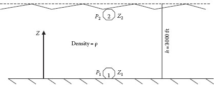
Note that the diagram has been labeled with the pertinent reference points (1, 2), pressures (P) and elevations (Z) at these points, the depth (h), and the water density (ρ).
Assumptions: We will make the following assumptions:
1. The sea water is an incompressible (constant density) liquid with ρ = 64 lbm/ft3.
2. The surface of the ocean and the sea bottom are flat.
3. The barometric pressure is exactly 1 atm.
It should be noted that none of these assumptions is exact, but they should be adequate to obtain a reasonable answer.
Theory: The theoretical expression that relates the pressure in an incompressible fluid to the elevation in the fluid is derived in Chapter 4 and is expressed as
Note that once the correct theoretical expression is identified, pertinent variables and parameters can be identified from the terms in the equation and used to complete the labeling of the diagram.
Apply theory: We must tailor the general theoretical expression to the specific problem at hand:
Complete the solution: Now solve the equation for the desired quantity, insert values of known quantities with conversion factors as required (noting that h = Z2 − Z1), and calculate the answer:
Note that the answer has been rounded to three digits or significant figures. This should be consistent with the probable precision of the data (e.g., ρ and h) used to calculate the answers, in light of the assumptions made. Conversion factors and significant digits are discussed in detail in Chapter 2.
III. PHENOMENOLOGICAL RATE OR TRANSPORT LAWS
In addition to the laws for the conservation of mass, energy, momentum, etc. there are additional physical laws that govern the rate at which these conserved quantities are transported from one region to another in a continuous medium. These are called phenomenological laws because they are based on observable phenomena and logical deduction but they cannot be derived from first principles. These “rate” or “transport” models can be written for any conserved quantity (mass, energy, momentum, electric charge, etc.) and can be expressed in a general form as
1.1 |
This expression can be applied to the transport of any conserved (extensive) quantity “Q,” for example, mass, energy, momentum, electric charge, etc. The rate of transport of Q per unit area normal to the direction of transport is called the flux of Q, with dimensions of “Q”/(time × area). This transport equation can be applied on a microscopic scale in a stationary medium or to a fluid in motion. The moving fluid can be in laminar flow in which the mechanism for the transport of Q is the intermolecular forces of attraction between molecules or groups of molecules, or in turbulent flow in which the transport mechanism is the result of the motion of turbulent eddies which move in three dimensions and carry Q along with them. The resistance or conductance term in Equation 1.1 is also called the transport coefficient. For laminar or stationary media, the transport coefficient is a fluid or material property, but for turbulent flows it also depends upon the degree of turbulence in the medium.
On the microscopic or molecular level (e.g., stationary media or laminar flow), the driving force for the transport of Q in any direction (e.g., the y direction) is the negative of the concentration gradient of Q in that (y) direction. That is, Q flows “downhill,” from a region of high concentration to a region of low concentration, and the rate of transport of Q is proportional to the change in the concentration of Q divided by the distance over which it changes. At any specific point in the system, this can be expressed as
(1.2) |
where Kt is the transport coefficient for the quantity Q and CQ is the concentration of Q. For microscopic (molecular) transport, Kt is a property only of the medium, which is assumed to be a continuum, that is, all relevant physical properties can be defined at each and every point within the medium. This means that the smallest region of practical interest must be very large relative to the size of the individual molecules (or the distance between them) or any substructure of the medium such as particles, drops, bubbles, etc. It is further assumed that these properties are homogeneous and isotropic (i.e., they are the same at all points within the medium and are independent of direction). For macroscopic systems involving turbulent convective transport, the driving force is a representative difference in the concentration of Q, and the transport coefficient includes the effective distance (δ) over which this concentration changes, for example,
(1.3) |
where the transport coefficient is now (Kt/δ) and is dependent upon the flow conditions as well as properties of the medium. Note the absence of the minus sign on the right-hand side (RHS) of Equation 1.3. This is because the concentration change (ΔCQ) is generally interpreted as the magnitude of the change in concentration along the path of increasing y.
Example 1.2
What are the dimensions of the transport coefficient Kt?
Analysis: “Dimensions” represent the “physical character” of a given quantity (e.g., mass [M], length [L], time [t], etc.) (a complete discussion of units and dimensions is given in detail in Chapter 2). The “conservation of dimensions” or fruit salad law requires that all terms in any valid equation must have the same net dimensions. By applying this “law” to Equation 1.2 that defines the coefficient Kt, we can deduce the dimensions of Kt from the dimensions of the other terms in the equation.
Solution:
Denoting dimensions by square brackets (i.e., “the dimensions of x = [x]”), the dimensions of each term in Equation 1.2 are
Thus, the “dimensional” form of Equation 1.2 is
Since the dimensions of Q cancel out, the dimensions of Kt are L2/t, or
By similar reasoning, the dimensions of the coefficient (Kt/δ) are seen to be L/t.
A. FOURIER’s LAW OF HEAT CONDUCTION
Figure 1.1 illustrates two horizontal parallel plates with a uniform “medium” (either solid or fluid) in between. If the top plate is kept at a temperature T1 that is higher than the temperature T0 of the bottom plate, there will be transport of thermal energy (heat) from the upper plate to the lower plate through the medium, in the −y direction. If the flux of heat in the y direction is denoted by qy, then the corresponding transport law can be written as
(1.4) |
where
αT is the thermal diffusion coefficient, with dimensions of L2 t−1
(ρcvT) is the “concentration of thermal energy (heat)”
Because the density (ρ) and the heat capacity (cv) are assumed to be independent of position, this equation can be rewritten in the following form:
(1.5) |
where k = αTρcv is the thermal conductivity of the medium. The two forms of the equation on the right follow from the fact that the gradient (derivative) term is constant in the geometry of Figure 1.1. This is not true in general but is valid for this geometry and for any continuum in which the reference locations are sufficiently close together. Note that qy is negative because heat is being transported in the “−y” direction, from high temperature to low temperature. This law was formulated by Fourier in 1822 and is known as Fourier’s law of heat conduction. This law applies to stationary solids or fluids and to fluids moving in the x direction with straight streamlines (e.g., laminar flow).
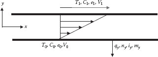
FIGURE 1.1 Transport of energy, mass, charge, and momentum from the upper surface to the lower surface.
An analogous situation can be envisioned if the medium is stationary (or is a fluid in laminar flow in the x direction) and the temperature difference (T1 − To) is replaced by the concentration difference (C1 − Co) of a substance that is soluble in the fluid (e.g., a top plate made of pure salt in contact with water). If the soluble species (e.g., the salt) is denoted by A, it will diffuse through the medium (B) from the high concentration C1 at the top plate to the low concentration Co at the bottom plate. If the flux of species A in the y direction is denoted by nAy, then the transport law is given by
(1.6) |
where DAB is the molecular diffusivity of species A in the medium B. Here, nAy is negative because species A is diffusing in the −y direction. Equation 1.6 is known as Fick’s law of diffusion and was formulated in 1855 (note that it is exactly the same as Fourier’s law, with just the symbols changed). In fact, both the molecular diffusivity DAB and the thermal diffusivity αT have identical dimensions of L2 t−1.
C. OHM’s LAW OF ELECTRICAL CONDUCTIVITY
The same transport law can be written for electric charge (which is another conserved quantity). In this case, the top plate in Figure 1.1 is assumed to be at an electric potential of e1 which is higher than the potential e0 at the bottom plate (note: “electric potential” is equivalent to “concentration of electric charge” or voltage). The corresponding “charge flux,” i.e., “current density,” in the y direction is iy, which is negative because the charge transport is in the −y direction. The corresponding expression for the charge flux is known as Ohm’s law (1827) and is written as
(1.7) |
where ke is the electrical conductivity of the medium between the plates, with dimensions of L2 t−1.
Momentum is also a conserved quantity, and an equivalent transport law can be written for the transport (flux) of momentum. We must be careful here, however, because velocity and momentum are vector quantities as opposed to mass, energy, and charge, which are all scalars. Even though we may draw some analogies between these scalar quantities and the one-dimensional transport of vector components, these analogies do not hold in general for multidimensional systems or for complex geometries. However, the conditions depicted in Figure 1.1 are for simple one-dimensional transport, in which case we can include the transport of the x-component of linear momentum by analogy with the transport of scalar quantities.
In this case, we consider the top plate to be subject to a force in the x direction, causing it to move with a constant velocity V1 in the x direction, while the bottom plate is stationary (V0 = 0). There is x momentum associated with any given element of fluid of mass m moving in the x direction with velocity vx. This x momentum is mvx and the corresponding concentration of x momentum (i.e., momentum per unit volume) must be ρvx. If we denote the flux of this x momentum in the y direction by (τyx)mf, the transport expression is
(1.8) |
where v is called the kinematic viscosity, with dimensions of L2 t−1. It should be evident that (τyx)mf is negative because the faster moving fluid at the top drags the slower moving fluid along with it so that x momentum is transported in the −y direction by virtue of this fluid “drag.” Because the fluid is assumed to be homogeneous, the density is independent of position and the flux of x momentum in the −y direction can therefore be written as
(1.9) |
where μ = ρv is the viscosity (or sometimes the dynamic viscosity). Equation 1.9 is Newton’s law of viscosity and was formulated in 1687! It applies to so-called Newtonian fluids in laminar flow (non-Newtonian fluids and turbulent flows will be considered in later chapters).
1. Momentum Flux and Shear Stress
Both Newton’s law of viscosity and the conservation of momentum are related to Newton’s second law of motion, which is commonly written as Fx = max = d(mVx)/dt, that is, force is equivalent to a rate of change of momentum. For a fluid in steady flow (constant velocity), this is equivalent to Fx = ṁvx where ṁ is the fluid mass flow rate. Fx is the force acting in the x direction on the top plate in Figure 1.1, which makes it move, and it is also the driving force for the rate of transport of x momentum (ṁ Vx) from the faster to the slower moving fluid, in the −y direction. The flux of x momentum in the y direction (τyx)mf is therefore equivalent to the force Fx acting on unit area Ay. Note that “area” has both magnitude and direction due to the orientation of the surface and is thus a vector quantity with three components. The direction of the area vector is defined by the unit vector that is the outward normal to the surface that bounds the fluid volume of interest (i.e., the “system”). Because a surface has two sides and hence has both a “positive” and “negative” direction, the convention is that the surface bounding the volume element whose outward normal vector points in the positive direction is positive and the surface whose outward normal vector points in the negative direction is negative. In Figure 1.1, +Ay is the area of the surface bounding the fluid element in contact with the top plate (the “system”), which has an outward normal vector in the +y direction. The quantity Fx/Ay is also known as the shear stress, τyx, that acts on the fluid (i.e., it is the +Fx force, acting in the +x direction, on the area Ay of +y surface). It should be evident that, with reference to Figure 1.1, the momentum flux (τyx)mf is negative (+x momentum being transported in the −y direction), whereas the shear stress (τyx) is positive (+Fx force acting on +Ay surface), thus
(1.10) |
That is, the momentum flux is always the negative of the corresponding shear stress. In the field of mechanics, the “shear stress” sign convention is customary, as opposed to the “momentum flux” sign convention, and that is the one we will follow in this book. It is important to recognize the difference between these two sign conventions, because references that use the momentum flux convention define the viscosity of a Newtonian fluid by Equation 1.9, whereas if the shear stress convention is used, viscosity is defined by the equation
(1.11) |
The equations representing each of the preceding one-dimensional transport laws are all identical, except for the notation (e.g., “the game is the same—only the color of the jerseys is different”), and all of the transport coefficients (DAB, αT, ke, and v have the same dimensions, i.e., L2/t). However, there are some features of Newton’s law of viscosity that distinguish it from the other laws, which are important when applying this law. First, as previously mentioned, momentum is fundamentally different from the other conserved quantities in that it is a vector (with directional properties), whereas the others (mass, energy, electric charge) are scalars, independent of direction. Now, the gradient operator or “directional derivative” (d()/dy in one dimension or ∇() in more general 3D notation) is also a vector. It thus follows that the gradient of a scalar is a vector (i.e., the flux of heat, mass, or charge), and the gradient of a vector (e.g., velocity or momentum), and hence the flux of momentum (or stress), is a dyad or second-order tensor. Dyads are associated with two directions: the direction of the vector quantity and the direction in which it varies. Thus, (τyx)mf represents the flux of x momentum in the y direction. Likewise, the shear stress components (e.g., τyx), which represent a force (Fx) acting on an area component (Ay oriented normal to the y direction, are tensor components or dyads, with nine possible components. Again, recall that area is a vector because of its orientation, with a positive area being that which bounds the fluid element of interest with its outward normal vector pointing in the positive coordinate direction. In general, a 3D (x, y, z) space vector can be represented by three components, whereas a dyad or second-order tensor has nine possible components. This difference between momentum flux and the flux of a scalar quantity is very significant when applying the equations to 3D space or to path lines, which are not straight. In such cases, the analogy between Newton’s law of viscosity and the other transport laws is lost.
4. Newtonian and Non-Newtonian Fluids
Fluids that obey Newton’s law of viscosity are characterized by the fluid property “viscosity” (μ), which is assumed to be constant (i.e., independent of position, time, or flow conditions). This is true of the other transport properties for heat, mass, and electric charge as well, all of which are assumed to be dependent upon the thermodynamic state of the material (e.g., temperature, pressure, density) but independent of the “dynamic” state, that is, the state of stress or deformation. Many common fluids are Newtonian, although there are many fluids for which this assumption is not true with respect to viscosity, and for these the viscosity does depend upon the state of stress or deformation and hence is a function of the dynamic state of the fluid. Gases, low molecular weight simple inorganic and organic liquids and solutions of relatively low-molecular-weight compounds, molten metals, and salts all are examples of Newtonian fluid behavior. “Non-Newtonian” fluids are typically complex materials with significant “substructure,” such as melts or solutions of high-molecular-weight polymers, suspensions of solids in liquids, emulsions of liquids in liquids, foam suspensions of gas bubbles in liquids, surfactant solutions, etc. Typical examples are paint, ink, pastes, liquid soaps, blood, mud, ketchup, mayonnaise, mustard, milk shakes, creams, lotions, etc.
The characteristics of linear, nonlinear viscous, and viscoelastic fluids are discussed in Chapter 3, and an analysis of the flow characteristics of a variety of “purely viscous” non-Newtonian fluids is included in later chapters. However, a completely general treatment of the flow and deformation behavior of non-Newtonian (including viscoelastic) fluids is beyond the scope of this book, and for this the reader is referred to the more advanced literature (e.g., Darby, 1971; Carreau et al., 1997; Chhabra and Richardson, 2008). Nevertheless, quite a bit can be learned and many practical problems solved by considering relatively simple models for the non-Newtonian properties of some complex fluids, provided the complexities of viscoelastic behavior can be avoided. These properties can be measured in the laboratory, with proper attention to data interpretation, and can be represented by any of several relatively simple mathematical expressions such as those illustrated in Chapter 3 and the books cited above. We do not attempt to delve in detail into the molecular or structural properties of these complex fluids but will make use of information that can be readily obtained through routine measurements. In this context, the flow behavior of non-Newtonian fluids will be considered in parallel with Newtonian fluids wherever possible and within the framework of the continuum hypothesis.
Example 1.3
With respect to Figure 1.1, consider the two parallel flat surfaces spaced 1 mm apart, with a Newtonian grease between them that has a viscosity of 200 cP. If the area of the plates in contact with the grease is 1 m2, determine the force (in lbf) required to make the top plate move at a velocity of 1 ft/s when the bottom plate is stationary.
Analysis: Equation 1.11 applies here
We use the form on the far RHS because the gradient (dVx/dy) is constant, that is, the velocity varies linearly in the gap. Setting V0 and y0 equal to zero and τyx = Fx/Ay′ the equation can be rearranged to solve for Fx:
Inserting the given quantities with units and conversion factors, and noting that 200 cP = 2 P = 2 (g/cm s) = 2 (dyn s/cm2), gives
Note that the actual number of significant digits is indeterminate because all given values are whole numbers, which implies either “infinitely exact” values or unspecified precision. When in doubt about the number of significant digits to report in the answer, the rule of thumb is a maximum of three digits, unless more can be justified. Note that three significant digits implies a precision somewhere between 0.05% and 0.5%, which is better than that of most engineering data.
“I was told to measure twice with a micrometer, mark it with chalk, and then cut it with an axe.”
—Anonymous
The basic conservation laws, as well as the transport models, are generally applied to a specified region or volume of fluid designated as “the system” (sometimes called a “control volume”). The system is not actually the volume of the fluid container (e.g., a tank, pipe, pump, etc.) but is the fluid within a defined region. For flow problems, there may be one or more streams entering and/or leaving the system, each of which can carry or transport a conserved quantity (e.g., Q) into and/or out of the system at a defined rate (Figure 1.2). Q may also be transported into or out of the system through the system boundaries by other means in addition to being carried by the in/out streams. The general conservation law for a flow problem with a defined system with respect to any conserved quantity Q can be written as
(1.12) |
If Q can be produced or consumed within the system (e.g., through a chemical or nuclear reaction, speeds approaching the speed of light, etc.), then a “rate of generation” term can be included on the left of Equation 1.12. However, these effects will not be significant in the systems with which we are concerned. The system in Figure 1.2, for example, would be the material (fluid) between the parallel plates. There are no “in” or “out” streams in this example, but the conserved quantity is transported into the system by microscopic (molecular) interactions through the upper boundary of the system. These and related concepts will be expanded upon in Chapter 5 and succeeding chapters.
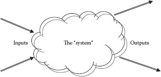
FIGURE 1.2 The “system.”
V. TURBULENT MACROSCOPIC (CONVECTIVE) TRANSPORT MODELS
The transport expressions illustrated in Equations 1.5 through 1.7 and 1.9 apply to the transport of heat, mass, charge, or momentum from one region of the continuum to another by virtue of molecular interactions only. That is, there is no actual bulk motion of the material in the transport direction (y), which means that the medium must be stationary or moving only in the direction normal to the direction of the transport (x). Consequently, the flow must be laminar, that is, all elements move in straight parallel streamlines in the x direction. This occurs only if the velocity is sufficiently low so that it is dominated by stabilizing viscous forces. However, as the velocity increases, destabilizing inertial forces eventually overcome the viscous forces and the flow becomes turbulent. Turbulence produces a 3D fluctuating flow field dominated by “eddies” that produce a high degree of mixing or “convection” due to the bulk motion of these eddies. As a result, the flow is highly mixed, except for a region in the immediate vicinity of the solid boundary that is called the boundary layer (thickness δ). As the fluid velocity must be zero at a stationary boundary, there must be a region (boundary layer) adjacent to the wall which is laminar. Consequently, the major resistance to transport in turbulent (convective) flows is within this boundary layer, the size of which depends upon the dynamic state of the flow field, as well as the fluid and solid properties. As the distance from the wall increases, this laminar boundary layer will transition to a turbulent boundary layer with a thickness that depends on the intensity of the turbulence in the main flow field. This turbulent boundary layer thickness is typically small compared to the total dimensions of the flow field (see Chapter 6 for more detail on this subject).
The general turbulent transport models for the transport of heat and mass are
(1.13) |
(1.14) |
where
ke is a turbulent or “eddy thermal conductivity”
h is the heat transfer coefficient
De is the “eddy diffusivity”
Km is the mass transfer coefficient
The situation with regard to convective (turbulent) momentum transport is somewhat more complex because of the tensorial character of momentum flux (or stress). As previously explained, Newton’s second law provides a correspondence between a force Fx (acting in the x direction) and the rate of transport of x momentum. For continuous steady flow in the x direction at a constant velocity Vx in a conduit of cross-sectional area Ax, there is transport of x momentum in the x direction, which is given by
(1.15) |
The corresponding flux of x momentum in the x direction is . This is also the driving force for the transport of x momentum in the −y direction (toward the wall), that is, τyx = Fx/Ay. Therefore, the convective flux of x momentum from the fluid to the wall (or the equivalent stress exerted by the fluid on the wall) can be expressed as
(1.16) |
where f is the Fanning friction factor. The factor of 2 is arbitrary, and various other definitions of the friction factor vary from this by factors of 2 or 4 (see Chapter 6). Although Equation 1.16 is the counterpart of Equations 1.13 and 1.14 for heat and mass, it appears somewhat different as a result of the correspondence between force and the rate of momentum, and the multidimensional (tensor) nature of stress and momentum flux. It is seen from Equation 1.11 that laminar flows are dominated by the fluid viscosity (which is stabilizing), and from Equation 1.16 that turbulent flows are dominated by the fluid density (i.e., inertial forces), which is destabilizing. A fundamental definition of f and its dependence on flow conditions and fluid properties, which is consistent for either laminar or turbulent flow, are discussed in Chapters 5 and 6. Because of the highly complex unsteady fluctuations in turbulent flows, the corresponding turbulent transport coefficients (i.e., h, Km, and f) cannot be predicted from fundamental principles and must be determined by experimental investigation and correlation.
Example 1.4
It can be argued that all physical quantities have the mathematical properties of a “tensor,” when the latter is defined in terms of the number of directions associated with the quantity. For example, a scalar can be described as a “zero-order tensor,” as it has magnitude only, but zero directions associated with it; a vector is a “first-order tensor” as it has a magnitude and one direction; a dyad is a “second-order tensor,” with a magnitude and two directions, etc.
(a) With regard to the fluid contained between two parallel plates illustrated in Figure 1.1, identify the “tensorial order” and directional character of each of the transported quantities associated with the fluid.
(b) Considering an extension of the “vector” and “tensor (dyad)” character of these quantities, can you think of a physical quantity that can be described as a third-order tensor (e.g., a triad)?
Solution:
(a) The transported quantities are heat, mass, electric charge, and momentum. Each of these quantities is measured by an intensive variable that indicates the “concentration” of that quantity, per unit mass of the medium (e.g., temperature, concentration, voltage or potential, and velocity). All of these quantities, and their intensive variables, are scalars (“zero-order tensors”) except momentum (velocity), which is a “first-order tensor” (vector) with magnitude and one direction.
(b) The rate of transport of these quantities is proportional to the rate at which the concentration of that quantity (as represented by its intensive property) changes with direction, that is, it is “concentration gradient.” It can be observed that the “gradient” of a quantity adds an additional direction to that quantity, as the gradient represents the magnitude and direction of the change of that quantity and hence is a “gradient vector.” Hence, the gradient of each of the scalars (heat/temperature, mass/concentration, electric charge/potential) is a vector, and the gradient of a vector (e.g., momentum/velocity) is a second- order tensor (dyad). By extension, the gradient of a dyad (momentum flux or stress) must be a “triad” or “third-order tensor,” that is, the rate at which “stress” (components) varies with position, or the “stress gradient” must be a triad. In principle, this concept can be extended indefinitely.
The key points covered in this chapter include:
• A basic understanding of quantities that are “conserved”in engineering systems (e.g., mass, energy, momentum, electric charge, “dimensions,” and “dollars”);
• The equations defining fundamental laws that govern the rate of transport of these conserved quantities in a dynamic system by both microscopic (molecular) and macroscopic (convective) mechanisms (e.g., Fourier’s law, Fick’s law, Ohm’s law, Newton’s law of viscosity, and the turbulent convective transport coefficients for mass, heat, and momentum);
• The concepts of force and momentum and their relationship to stress and momentum flux;
• The concept of a system as the reference or control volume to which the conservation equations are applied;
• The significance of tensors versus vectors and scalars with respect to conserved and transported quantities;
• The “4 C’s” guidelines for effective problem solving and the importance of “experience” and “judgment” in the practice of engineering.
1. Write the general 3D equations for the definitions of each of the following laws: Fick’s, Fourier’s, Ohm’s, and Newton’s laws. Identify the conserved quantity in each of these laws. Can you represent all of these laws by the same generalized expression? If so, does that mean that all of these processes are always analogous? If not, why not?
2. The general expression for the conservation of any (conserved) quantity Q can be written in the form of Equation 1.12. We have said that “dollars” are also a conserved quantity, so Equation 1.12 should apply. Substituting “$” for Q in this equation and assuming that the “system” is your bank account:
(a) Identify specific items that correspond to “rate in” and “rate out” and “rate of accumulation” with respect to your “system” (i.e., each term should correspond to the rate at which dollars move into or out of your account).
(b) Identify one or more “driving force” effects that govern each of these rate terms, that is, the things that influence how fast the dollars go in or out. Use this to define respective “transport coefficients” relating the “driving force” and the “rate” for each term in the equation.
3. A dimensionless grouping of variables and parameters that are important in pipe flow is called the Reynolds number:
where
V is the average velocity over the cross section in a pipe of diameter D
ρ is the fluid density
μ is the fluid viscosity
Comparing the numerator and denominator of the RHS of the equation with Equations 1.16 and 1.11 shows that this group is a ratio of the convective (turbulent) momentum flux to the laminar (viscous) momentum flux, or the ratio of (destabilizing) inertia forces to (stabilizing) viscous forces. Thus, at low values of the Reynolds number, viscous forces dominate and the flow is smooth and stable (laminar), and at high Reynolds numbers, inertial forces dominate and the flow is unstable (turbulent). It has been found that laminar flow occurs in a pipe only when the Reynolds number is less than about 2000. Calculate the maximum velocity and the corresponding volumetric flow rate (in cm3/s) at which laminar flow of air and water is possible in pipes with the following diameters:
4. A layer of water is flowing down a flat plate that is inclined at an angle of 20° to the vertical. If the depth of the layer is ¼ in., what is the shear stress exerted by the plate on the water? (Remember: stress is a dyad, with two directions associated with each component.)
5. The relationship between the forces and fluid velocity can easily be illustrated by considering the simple one-dimensional steady flow between two parallel plates, Figure 1.1. The area of each plate Ay = 1 m2 and the gap between the two plates is 0.1 mm (very thin). Fluids of different viscosities, as listed below, are contained in between the two plates. A tangential force of 1 N is applied to the top plate moving in the x direction at a fixed velocity V0 while the bottom plate is held stationary. Calculate the value of V0 for each of the following fluids:
Substance |
Viscosity (cP) |
Olive oil |
100 |
Castor oil |
600 |
Pure glycerin (293 K) |
1500 |
Honey |
104 |
Corn syrup |
105 |
Bitumen |
1011 |
Molten glass |
1015 |
In view of these results, what is the meaning of the phrase from the Bible: “the mountains flowed before the Lord” and the significance of the phrase: “Everything flows”!
6. A slider bearing consists of a sleeve surrounding a cylindrical shaft that is free to move axially within the sleeve. A lubricant (e.g., grease) is in the gap between the shaft and the sleeve to isolate the metal surfaces and support the stress resulting from the motion of the shaft. The diameter of the shaft is 1 in. and the inside diameter of the sleeve is 1.02 in., and its length is 2 in.
(a) If you want to limit the total force on the sleeve to less than 0.5 lbf when the shaft is moving with a velocity of 20 ft/s, what should the viscosity of the grease be, in centipoise?
(b) If the grease has a viscosity of 400 cP (centipoise), what is the force exerted on the sleeve when the shaft is moving at a velocity of 20 ft/s?
(c) The sleeve is cooled to a temperature of 150°F, and it is desired to keep the shaft temperature below 200°F. What is the cooling rate (i.e., the rate at which heat must be removed through the sleeve by the coolant, in Btu/h), to achieve this temperature? The properties of the grease are as follows: specific heat = 0.5 Btu/lbm°F, specific gravity (SG) = 0.85, thermal conductivity = 0.06 Btu/h ft °F.
(d) If the grease becomes contaminated, it could be corrosive to the shaft metal. Assume that this occurs and the surface of the shaft starts to corrode at a rate of 0.1 μm/year. If this corrosion rate is constant, determine the maximum concentration of metal ions in the grease when the ions from the shaft just reach the sleeve. The properties of the shaft metal are as follows: molecular weight (MW) = 65, SG = 8.5, diffusivity of metal ions in grease = 8.5 × 10⁻⁵ cm2/s.
7. By making use of the analogies between the various transport models for molecular transport of conserved quantities, describe how you would set up an experiment to solve each of the following problems by making electrical measurements of voltage and current (e.g., describe the design of the experiment, how and where you would measure current and/or voltage, and how the measurements would be related to the desired quantity).
(a) Determine the rate of heat transfer from a long cylinder to a fluid flowing normal to the cylinder axis, if the surface temperature of the cylinder is T0 and the fluid temperature far away from the cylinder is T1. Determine also the temperature distribution within the fluid and the cylinder.
(b) Determine the rate at which a (spherical) mothball evaporates when it is immersed in stagnant air, and also the concentration distribution of the evaporating compound in the air.
(c) Determine the local stress as a function of position on the surface of a wedge-shaped body immersed in a fluid that is flowing slowly parallel to the surface. Determine also the local velocity distribution in the fluid as a function of position.
8. What is the “system” in Example 1.3?
9. Explain the “fruit salad law,” and how does it apply to the formulation of equations describing engineering systems?
A |
Area, [L2] |
Ay |
Area component whose normal vector is in the y direction, [L2] |
C |
Concentration of soluble species, [M/L3] |
CA |
Concentration of species A, [M/L3] |
cv |
Heat capacity at constant volume, [H/MT] |
D |
Pipe diameter, [L] |
DAB |
Diffusivity of species A in medium B, [L2/t] |
De |
Eddy diffusivity, [L2/t] |
e |
Electric potential (concentration of charge), [C/L2] |
f |
Pipe Fanning friction factor, [—] |
Fx |
Component of force in x direction, [ML/t2] |
g |
Acceleration due to gravity, [L/t2] |
h |
Depth, [L] |
h |
Heat transfer coefficient, [H/L2tT] |
k |
Thermal conductivity, [H/LtT] |
ke |
Electrical conductivity, [L2/t] |
Km |
Mass transfer coefficient, [L/t] |
KT |
General transport coefficient, [L2/t] |
iy |
Flux of charge (current density), [C/L2t] |
k |
Thermal conductivity, [H/LTt] |
L |
Length, [L] |
m |
Mass, [M] |
ṁ |
Mass flow rate, [M/t] |
nAy |
Flux of species A in the y direction, [M/L2t] |
NRe |
Reynolds number, [—] |
P |
Pressure, [M/Lt2] |
Q |
Generic notation for any conserved (or transported) quantity, [varies] |
qy |
Flux of heat in the y direction, per unit area normal to the y direction, [H/L2t] |
t |
Time, [t] |
T |
Temperature, [K or °R] |
vx |
Local or point velocity in the x direction, [L/t] |
V |
Spatial average velocity or velocity of a boundary, [L/t] |
X |
Coordinate direction, [L] |
x, y, z |
Coordinate directions, [L] |
z |
Elevation [L] |
GREEK
αT |
Thermal diffusivity (= ρcvT), [L2/t] |
δ |
Boundary layer thickness, [L] |
ρ |
Density, [M/L3] |
μ |
Viscosity, [M/Lt] = [Ft/L2] |
(τyx)mf |
Flux of x momentum in the y direction (= −τyx), [M/Lt2] = [F/L2] |
τyx |
Shear stress component = (force in x direction)/(area of y surface) = −(τyx)mf, [M/Lt2] = [F/L2] |
v |
Kinematic viscosity (= μ/p), [L2/t] |
Φ |
Potential, [F/L2] |
SUBSCRIPTS
mf |
Momentum flux, [M/Lt2] = [F/L2] |
0,1 |
locations 0,1 |
Carreau, P.J., D. Dekee, and R.P. Chhabra, Rheology of Polymeric Systems: Principles and Applications, Hanser, New York, 1997.
Chhabra, R.P. and J.F. Richardson, Non-Newtonian Flow and Applied Rheology, 2nd edn., Butterworth-Heinemenn, Oxford, U.K., 2008.
Darby, R., Viscoelastic Fluids, Marcel Dekker, New York, 1976.
* The “fruit salad law” states that you “can’t add apples and oranges unless you want fruit salad.”
* Dimensions given in brackets are as follows: L = length, M = mass, t = time, T = temperature, C = charge, H = “heat” = thermal energy = ML2/T2 (see Chapter 2 for discussion of units and dimensions).