2	Dimensional Analysis and Scale-Up

“Today’s scientists have substituted mathematics for experiments, and they wander off through equation after equation, and eventually build a structure which has no relation to reality.”

—Nikola Tesla, 1856–1943, Inventor

I.    INTRODUCTION

In this chapter, we consider various aspects of dimensions and units and the different systems in use for describing these quantities. In particular, the distinction between scientific and engineering systems of dimensions is explained, and the various metric and English* units used in each system are discussed. It is important that the engineer be familiar with both English and metric systems, as they are all in common use in various fields of engineering and will continue to be for the indefinite future. It is common to encounter a variety of units in different systems during the analysis of a given problem, and the engineer must be adept at dealing with all of them.

The concept of conservation of dimensions will be applied to the dimensional analysis and scale-up of engineering systems. It will be shown how these principles may be used in the design and interpretation of laboratory experiments on “model” or “prototype” systems to predict the behavior of large-scale (“field” or “real”) systems (this process is also known as similitude). These concepts are presented early on, because we shall make frequent use of them in describing the results of both theoretical and experimental analyses of engineering systems in a form that is the most concise, general, and useful. These methods can also provide guidance in choosing the best approach to follow in the solution of many complex problems.

II.    UNITS AND DIMENSIONS

A.    DIMENSIONS

The dimensions of a quantity identify the physical character of that quantity, for example, force (F), mass (M), length (L), time (t), temperature (T), electric charge (e), etc. On the other hand, units identify the reference scale by which the magnitude of the respective physical quantity is measured. Many different reference scales (units) can be defined for a given dimension; for example, the dimension of length can be measured in units of miles, centimeters, inches, meters, yards, angstroms, furlongs, light years, kilometers, etc. Dimensions can be classified as either fundamental or derived. Fundamental dimensions are those that cannot be expressed in terms of any other dimensions and include length (L), time (t), temperature (T), mass (M), and/or force (F) (depending upon the system of dimensions used). Derived dimensions can be expressed in terms of fundamental dimensions. Using the notation that “[x] = the dimensions of x,” we see, for example, that area ([A] = L²), volume ([V] = L³), energy ([E] = FL = ML²/t²), power ([HP] = FL/t = ML²/t³), viscosity([μ] = Ft/L² = M/Lt), thermal conductivity ([k] = ML/t³T), etc. are all “derived”dimensions that can be expressed in terms of fundamental dimensions.

There are two systems of fundamental dimensions in use (with their associated systems of units). These can be referred to as scientific and engineering systems. These systems differ basically in the manner in which the dimension of force is defined. In both systems, mass, length, and time are fundamental dimensions. Furthermore, Newton’s second law provides a relation between the dimensions of force, mass, length, and time:

$\text{Force = mass × acceleration}$

that is,

$F=ma$

(2.1)

or

$\left[F\right]=\left[ma\right]={\text{ML/t}}^2$

In scientific systems, this is accepted as the definition of force; that is, force is a derived dimension, being identical to ML/t².

In engineering systems, however, force is considered in a more practical or “pragmatic” context. This is because the mass of a body is not usually measured directly but is instead determined by its “weight” (W), that is, the gravitational force resulting from the mutual attraction between two bodies of mass m₁ and m₂:

$W=G\frac{m_1{m}_2}{r^2}$

(2.2)

where

G is a constant having a value of 6.67 × 10⁻¹¹ N m²/kg²

r is the distance between the centers of masses m₁ and m₂

If m₂ is the mass of the earth, for example, and r is its radius at a certain location on earth, then W is the weight of mass m₁ at that location:

$W=m_{1}g$

(2.3)

The quantity g is called the acceleration due to gravity and is equal to Gm₂/r² where G is a constant. On the earth at sea level and 45° latitude (the condition for standard gravity), the value of g is 32.174 ft/s² or 9.806 m/s². The value of g is obviously different on the moon (different r and m₂), and also varies slightly over the surface of the earth as well (since the radius of the earth varies with both elevation and latitude).

Since the mass of a body is determined indirectly by measuring its weight (i.e., the gravitational force acting on the mass) under specified gravitational conditions, engineers decided that it would be more practical and convenient if a system of dimensions were defined in which “what you see is what you get,” that is, the numerical magnitudes of mass and weight are equal under standard conditions. This must not violate Newton’s law, however, so that both Equations 2.1 and 2.3 are valid. Since the value of g is not unity when expressed in common units of length and time, the only way to have the numerical values of weight and mass be the same under any conditions is to introduce a “conversion factor” that forces this equivalence. This factor is designated g_c and is incorporated into Newton’s second law for engineering systems (sometimes referred to as “gravitational systems”) as follows:

$F=\frac{ma}{g_c},W=\frac{mg}{g_c}$

(2.4)

This additional definition of force is equivalent to treating F as a fundamental dimension, in addition to mass (m), the redundancy being accounted for by the conversion factor g_c. Thus, if a unit for the weight of mass m is defined so that the numerical values of F and m are identical under standard gravity conditions (i.e., a = g_std = 32.174 ft/s²), it follows that the numerical magnitude of g_c must be identical to that of g_std so that their magnitudes cancel out in Equation 2.4. However, it is important to distinguish between g (ft/s²) and g_c (ft lb_m/lb_f s²), because they are fundamentally different quantities. As explained earlier, g is not a constant—it is a variable that depends on both m₂ and r (Equation 2.2). However, g_c is a constant, because it is merely a conversion factor that is defined by the value of standard gravity. Note that these two quantities are also physically different, because they have different dimensions as well as different units:

$\left[g\right]=\frac{L}{{\text{t}}^2},\left[g_c\right]=\frac{\text{ML}}{{\text{Ft}}^2}$

(2.5)

The factor g_c is the conversion factor that relates equivalent force and mass units in engineering systems. In these systems, both force and mass can be considered fundamental dimensions, because they are related by two separate (but compatible) definitions: Newton’s second law and the definition of weight. The conversion factor g_c thus accounts for the redundancy in these two definitions.

B.    UNITS

Several different sets of units are in use in both scientific and engineering systems of dimensions. These can be classified as either metric (SI and cgs) or English (fps). Although the internationally accepted standard is the SI scientific system, English engineering* units are still very common in the United States and will probably remain so for the foreseeable future. Therefore, the reader should master at least these two systems and become adept at converting between them. These systems are illustrated in Table 2.1.

TABLE 2.1

Systems of Dimensions/Units

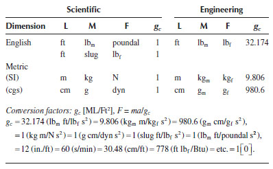
Note that there are two different English scientific systems, one in which M, L, and t are fundamental and F is derived, and another in which F, L, and t are fundamental and M is derived. In the system in which mass is fundamental, the unit for mass is the slug, and for the system in which force is fundamental, the force unit is the poundal. However, these systems are archaic and rarely used in practice. Also, the metric engineering systems with units of kg_f and g_f have generally been replaced by the SI system, although they are still in use in some places. The most common systems in general use are the scientific metric (e.g., SI) and the English engineering (or American) systems.

Since Newton’s second law is satisfied identically in scientific units with no conversion factor (i.e., g_c = 1), the following identities hold:

$\begin{array}{l}{g}_c=1\text{kg}\text{m/N}{\text{s}}^2=1\text{g}\text{cm/dyn}{\text{s}}^2=1\text{slug}{\text{ft/lb}}_{\text{f}}{\text{s}}^2=1{\text{lb}}_{\text{m}}\text{ft/poundal}{\text{s}}^2,\hfill \\ g_c=1\text{kg}\text{m/N}{\text{s}}^2=1.\hfill \end{array}$

In summary, in engineering systems both F and M are considered fundamental dimensions because of the engineering definition of weight, in addition to Newton’s second law. However, this apparent redundancy is rectified by the conversion factor g_c. The value of this conversion factor in the various engineering units provides the following identities:

$g_c=9.806{\text{kg}}_{\text{m}}{\text{m/kg}}_{\text{f}}{\text{s}}^2=980.6{\text{g}}_{\text{m}}{\text{cm/g}}_{\text{f}}{\text{s}}^2=32.174{\text{lb}}_{\text{m}}{\text{ft/lb}}_{\text{f}}{\text{s}}^2.$

C.    CONVERSION FACTORS

Conversion factors relate the magnitudes of different units with common dimensions and are actually identities; that is, 1 ft is identical to 12 in., 1 Btu is identical to 778 ft lb_f, etc. Because any identity can be expressed as a ratio with a magnitude and no net dimensions, the same holds for any conversion factor, that is,

$12\text{in}\text{./ft=778}\text{ft}{\text{lb}}_{\text{f}}\text{/Btu}\text{=}\text{30}\text{.48}\text{cm/ft}\text{=}\text{14}\text{.7}\text{psi/atm}{\text{=10}}^3\text{dyn/N}\text{=}\text{1}\left[0\right].$

A table of commonly encountered conversion factors is included in the “Unit Conversion Factors” front matter of this book. The value of any quantity expressed in a given set of units can be converted to any other equivalent set of units by multiplying or dividing by the appropriate conversion factor in the table to cancel the unwanted units.

Note that the conversion factor relating mass units in scientific systems to those in engineering systems can be obtained by equating the appropriate values of g_c from the two systems, for example,

$g_c=1\text{slug}{\text{ft/lb}}_{\text{f}}{\text{s}}^2=32.174{\text{lb}}_{\text{m}}{\text{ft/lb}}_{\text{f}}{\text{s}}^2.$

Thus, after canceling common units, the conversion factor relating slugs to lb_m is $\begin{array}{|c|}\hline 32.174l{b}_m/slug.\\ \hline\end{array}$

III.    CONSERVATION OF DIMENSIONS

Physical laws, theories, empirical relations, etc., are expressed by equations that relate the various variables and parameters. These equations usually contain a number of terms—for example, when a projectile is fired from a gun, the relation between the vertical elevation (z) of the projectile and its horizontal distance (x) from the gun at any time can be expressed in the form

$z=ax+b{x}^2$

(2.6)

This equation can be derived from the laws of physics, and in the process the parameters a and b are related to such factors as the muzzle velocity, projectile mass, angle of inclination of the gun, wind resistance, etc. The equation may also be empirical if measured values of z versus x can be fit by an equation of this form, with no reference to the laws of physics. For any equation to be valid, every term in the equation must have the same physical character, that is, the same net dimensions, and consequently the same units in any consistent system of units. This is known as the law of conservation of dimensions (otherwise known as the “fruit salad law”—“you can’t add apples and oranges, unless you are making fruit salad”). Let us look further at Equation 2.6. Since both z and x have dimensions of length, for example, [x] = L, [z] = L, it follows from the fruit salad law that the dimensions of a and b must be

$\left[a\right]=0,\left[b\right]=1/\text{L}$

that is, a has no dimensions (it is dimensionless) and the dimensions of b are 1/L, or L⁻¹. For the sake of argument, let us assume that x and z are measured in feet and that the values of a and b in the equation are 5 and 10 ft⁻¹, respectively. Thus, if x = 1 ft,

$z=\left(5\right)\left(1\text{ft}\right)+\left(10{\text{ft}}^{-1}\right){\left(1\text{ft}\right)}^2=15\text{ft}$

(2.7)

On the other hand, if we choose to measure x and z in inches, the value of z for x = 1 in. is

$z=\left(5\right)\left(1\text{in}\text{.}\right)+\left(10{\text{ft}}^{-1}\right)\left(\frac{1}{12}\text{ft/in}\text{.}\right){\left(1\text{in}.\right)}^2=5.83\text{in}.$

(2.8)

This is still in the form of Equation 2.6, that is,

$z=ax+b{x}^2,$

but now a = 5 and b = 10/12 = 0.833 in.⁻¹. Thus, the magnitude of a has not changed, but the magnitude of b has changed. This simple example illustrates two important principles:

1.  Conservation of dimensions (“fruit salad” law): All terms in a given equation must have the same net dimensions and consistent units for the equation to be valid.

2.  Scaling: The fact that the value of the dimensionless parameter a is the same regardless of the units (e.g., scale) used in the problem illustrates the universal nature of dimensionless quantities. That is, the magnitude of any dimensionless quantity will always be independent of the scale of the problem or the units used. This is the basis for the application of dimensional analysis, which permits information and relationships determined in a small-scale system (e.g., a prototype or “model”) to be applied directly to a similar system of a different size or scale if the system variables are expressed in dimensionless form. This process is known as “scale-up.”

The universality of certain dimensionless quantities is often taken for granted. For example, the exponent 2 in the last term of Equation 2.6 has no dimensions and hence has the same magnitude regardless of the scale or units used for measurement. Likewise, the kinetic energy per unit mass of a body moving with a velocity V is given by

$ke=\frac{V^2}{2}$

(2.9)

Both of the numerical quantities in this equation, 1/2 and 2, are dimensionless so they always have the same magnitude regardless of the units used to measure V.

A.    NUMERICAL VALUES

Ordinarily, numerical quantities that appear in equations that have a theoretical basis (such as the ke equation above) are dimensionless and hence “universal.” However, many valuable engineering relations have an empirical rather than a theoretical basis, in which case this conclusion does not always hold. For example, a very useful expression for the (dimensionless) friction loss coefficient (K_f) for valves and fittings that we will use later is

$K_f=\frac{K_1}{N_{Re}}+K_i\left(1+\frac{K_d}{D_{n\left(\text{in}.\right)}^{0.3}}\right)$

(2.10)

Here, N_Re is the Reynolds number, which is dimensionless, as are K_f and the constants K₁ and K_i. However, the term D_{n (in.)} is the nominal diameter of the fitting in inches, which has dimensions of length. According to the “fruit salad” law, the constant K_d in the term $K_d/D_{n\left(\text{in}.\right)}^{0.3}$ must therefore have dimensions of L^0.3 and so is not independent of scale, that is, its magnitude is defined only in specific units. In fact, as the magnitude of D_{n (in.)} is defined with units of in., K_d must also be expressed in units of in., for example, in.^0.3. If D_{n (in.)} were to be measured in centimeters, for example, the value of K_d would be 1.32 times as large, because [(1 in.)(2.54 cm/in.)]^0.3 = (2.54 cm)^0.3 = 1.32 cm^0.3. Therefore, caution must be exercised when using such empirical relations that are not in a dimensionless form or are not dimensionally consistent.

B.    CONSISTENT UNITS

The conclusion that dimensionless numerical values are universal is valid only if a consistent system of units is used for all quantities in a given expression. That is, units for all quantities with the same dimensions should always be the same and not “mixed,” that is, always using ft for the unit of length and not mixing ft and m in the same expression. If such is not the case, then the numerical quantities may include conversion factors that relate the different units. For example, the velocity (V) of a fluid flowing in a pipe is related to the volumetric flow rate (Q) and the internal pipe diameter (D) by the following “universal” equation with consistent units:

$V=\frac{4}{\pi }\frac{Q}{D^2}$

(2.11)

The dimensions must be the same on both sides of the equation, that is, [V] = L/t, [Q/D²] = (L³/t) (1/L²) = L/t, and if the units are consistent (e.g., all length dimensions in the same units), then the dimensionless numerical values (4 and π) are “universal,” with the same values regardless of the system of dimensions or units chosen. However, the following equations for V can also be found in various engineering reference books:

$V=183.3\frac{Q}{D^2}$

(2.12)

$V=0.408\frac{Q}{D^2}$

(2.13)

$V=0.286\frac{Q}{D^2}$

(2.14)

Although the dimensions of V and Q/D² are the same in each of these equations, it is evident that the numerical coefficient is not universal despite the fact that it must be dimensionless. This is because a consistent system of units is not used in these three equations. In each equation, the unit of V is ft/s and D is in in. However, in Equation 2.12, Q is in ft³/s, whereas in Equation 2.13, Q is in gallons per min (gpm), and in Equation 2.14, it is in barrels per hour (bbl/h). Thus, although the dimensions are consistent, the units are not, and therefore the numerical coefficients must include unit conversion factors. Only in Equation 2.11 are all the units assumed to be from the same consistent set (e.g., Q in ft³/s and D in ft), so that the factor 4/π is both dimensionless and unitless and is thus universal. It is always advisable to write equations in a universally valid form, where possible, to avoid confusion; that is, all quantities should be expressed in consistent units, and numerical values should be both dimensionless and unitless.

Let us consider another example to illustrate this point. The well-known Hazen–Williams formula for the flow of water in smooth pipes relates the volumetric flow rate (Q, in gpm) to the applied pressure gradient (ΔP/L, in psi/ft) and the pipe diameter (D, in in.) is

$Q=61.9D^{2.63}{\left(\frac{\Delta P}{L}\right)}^{0.54}$

(2.15)

When Equation 2.15 is rewritten in terms of the dimensions of each quantity, we get

$\left[{\text{L}}^{\text{3}}{\text{t}}^{-1}\right]={\left[\text{L}\right]}^{2.63}{\left[{\text{ML}}^{-2}{\text{t}}^{-2}\right]}^{0.54}$

or

$\left[{\text{L}}^{\text{3}}{\text{t}}^{-1}\right]={\left[\text{M}\right]}^{0.54}{\left[\text{L}\right]}^{1.55}{\left[\text{t}\right]}^{-1.08}$

2.16

The equation is clearly not dimensionally homogeneous and, therefore, the constant factor of 61.9 is not dimensionless. Thus, its value will change from one system of units to another, and this clearly does not make good sense.

IV.    DIMENSIONAL ANALYSIS

The law of conservation of dimensions can be applied to arrange all of the variables and parameters that are involved in a given problem into a set of dimensionless groups. The original set of (dimensional) variables can then be replaced by the resulting set of dimensionless groups as a new set of variables, and these can then be used in the equations or correlations that completely define the system behavior. That is, any valid relationship (theoretical or empirical) between the original variables can be expressed in terms of these dimensionless groups. This has two important advantages:

1.  Dimensionless quantities are universal (as we have seen), so any relationship involving dimensionless variables is independent of the size or scale of the system (including the fluid properties, as long as the fluid has the same rheological behavior, as discussed later, i. e., Newtonian or non-Newtonian [and described by the same rheological model], compressible or incompressible, etc.). Consequently, information obtained from a model (small-scale) system that can be represented in dimensionless form can be applied directly to geometrically and dynamically similar systems of any size or scale. This allows us to translate information directly from laboratory models to large-scale equipment or plant operations (scale-up). Geometrical similarity requires that the two systems have the same shape (geometry), and dynamic similarity requires them to be operating in the same dynamic regime (i.e., both must be in either laminar or turbulent flow). This will be expanded upon later.

2.  The number of dimensionless groups is always less than the number of original variables involved in the problem. Thus, the relations that define the behavior of a given system are much simpler when expressed in terms of the dimensionless groups as the variables, because fewer variables are required. In other words, the amount of effort required to represent a relationship between the dimensionless groups is much less than that required to relate each of the original variables independently, and so the resulting relation will be simpler in form. For example, a relation between two variables (x vs. y) requires two dimensions, whereas a relation between three variables (x vs. y vs. z) requires three dimensions, or a family of two-dimensional curves (e.g., a set of x vs. y curves, with each curve for a different z). This is equivalent to the difference between one page and a book of many pages. Relating four variables would obviously require many books or volumes and relating five variables would necessitate the entire library. Thus, reducing the number of variables from, say, four to two would dramatically simplify any problem involving these variables.

It is important to realize that the process of dimensional analysis only replaces the set of original (dimensional) variables with an equivalent (smaller) set of dimensionless variables (i.e., the dimensionless groups). It does not tell how these variables are related; the relationship must be determined either theoretically, by application of basic scientific principles, or empirically by measurements and data analysis. However, dimensional analysis is a very powerful tool in that it can provide a direct guide for experimental design and scale-up and for expressing operating relationships in the most general, simplified, and useful form in almost all branches of engineering, including living systems.

There are a number of different approaches to dimensional analysis. A classical method is the “Buckingham Π theorem,” so called because Buckingham used the symbol Π to represent the dimensionless groups.* Another classical approach, which involves a more direct application of the law of conservation of dimensions, is attributed to Lord Rayleigh. Numerous variations of these methods have also been presented in the literature. The one thing all of these methods have in common is that they require knowledge of the variables and parameters that are important in the problem as a starting point. This can be determined through common sense, logic, intuition, experience, physical reasoning, or by asking someone who is more experienced or knowledgeable. They can also be determined from knowledge of the physical principles that govern the system (e.g., the equations for the conservation of mass, energy, momentum, etc.), as written for the specific system to be analyzed. These equations may be macroscopic or microscopic (e.g., coupled sets of partial differential equations, along with their boundary conditions). The variables and parameters that appear in these governing equations, as well as in any relevant boundary conditions, constitute the set of relevant variables. However, this knowledge often requires as much (or more) insight, intuition, and/or experience than is required to compose the list of variables from logical deduction or intuition.

The analysis of any engineering problem requires key assumptions to distinguish those factors that are important in the problem from those that are insignificant. This can be referred to as the “bathwater” rule—it is necessary to separate the “baby” from the “bathwater” in any problem, that is, to retain the most significant elements (the “baby”) and discard the insignificant ones (the “bathwater”), and not vice versa! The talent required to do this depends much more upon sound understanding of fundamentals and the exercise of good judgment and intuition than upon mathematical facility, and the best engineer is most often the one who is able to make the most appropriate assumptions to simplify a problem (i.e., to discard the “bathwater” and retain the “baby”). Many problem statements, as well as solutions, involve assumptions that are implied but not stated. One should always be on the lookout for such implicit assumptions and try to identify them wherever possible since they may set corresponding limits on the applicability of the results.

The method we will use to illustrate the dimensional analysis process is one that involves a minimum of manipulations. It does require, as do all methods, an initial knowledge of the variables (and parameters) that are important in the system and the dimensions of these variables. At this stage, the omission of an important variable from the list of variables or inclusion of an irrelevant variable will obviously lead to an erroneous solution. Thus, compiling the list of relevant variables is germane to the success of this method. This step thus necessitates a good physical understanding of the problem at hand. The objective of the process is to determine an appropriate limited set of dimensionless groups of these variables that can then be used in place of the larger number of original individual variables for the purpose of simplifying the description of the system behavior. The process will be explained by means of an example, and the results will be used to illustrate the application of dimensional analysis to experimental design and scale-up.

A.    PIPELINE ANALYSIS

The procedure for performing a dimensional analysis will be illustrated by means of an example concerning the flow of a liquid through a circular pipe. In this example, we will determine an appropriate set of dimensionless groups that can be used to represent the relationship between the flow rate of an incompressible fluid in a pipeline, the properties of the fluid, the dimensions of the pipeline, and the driving force (pressure drop) for moving the fluid, as illustrated in Figure 2.1.

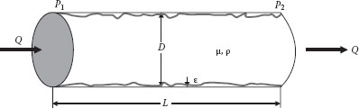
FIGURE 2.1 Flow in a pipeline.

The stepwise procedure is as follows:

Step 1: Identify the important variables. Most of the important fundamental variables in this system should be obvious and are labeled in Figure 2.1. By fundamental we mean that none of the variables should be related to others by definition. For example, the flow rate can be represented by either the total volumetric flow rate (Q) or the average velocity in the pipeline (V). However, these are related by the definition Q = πD²V/4, so if D is chosen as an important variable, then either V or Q can be chosen to represent the flow rate, but not both. We shall choose V. The driving force can be represented by ΔP, the difference between the pressure at the upstream end of the pipe (P₁) and that at the downstream end (P₂) (ΔP = P₁ − P₂), assuming the pipe to be horizontal. The pipe dimensions are the diameter (D) and length (L), and the fluid properties are the density (ρ) and viscosity (μ), assuming the fluid to be Newtonian. It is also possible that the “texture” of the pipe wall (i.e., the surface roughness ε) is important. This identification of the pertinent variables is the most important step in the process and can be done by using experience, judgment, brainstorming, and intuition or by examining the basic equations that describe the fundamental physical principles governing the system along with appropriate boundary conditions. For example, one might ask if surface tension and gravity are relevant here. It is also important to include only “fundamental” variables, that is, those that are not derivable from others through basic definitions. For example, as pointed out earlier, the fluid velocity (V), the pipe diameter (D), and the volumetric flow rate (Q) are related by the definition Q = πD²V/4. Thus, these three variables are not independent, since any one of them can be derived from the other two by this definition. It would therefore be necessary to include only two of the three.

Step 2: List all the problem variables and parameters, along with their dimensions. The procedure is simplest if the most fundamental dimensions in a scientific system (i.e., M, L, t) are used (e.g., force dimensions can be eliminated by utilizing a scientific system, energy can be converted to FL = ML²/t², etc.):

Variable	Dimensions
V	L/t
ΔP=(P1−P2)	F/L2 = M/(Lt2)
D	L
L	L
ε	L
p	M/L3
μ	M/(Lt)
Seven variables	Three dimensions

The number of dimensionless groups that will result from the analysis is equal to the number of variables less the minimum number of fundamental dimensions involved in these variables. Thus, there will be 7 − 3 = 4 groups in this problem. This is important, but this method does not tell us anything about what these groups are.

Step 3: Choose a set of reference variables. The choice of variables is arbitrary, except that the following criteria must be satisfied:

1.  The number of reference variables must be equal to the minimum number of fundamental dimensions in the problem (in this case, three).

2.  No two reference variables should have exactly the same dimensions.

3.  All the dimensions that appear in the problem variables must also be represented among the dimensions of the reference variables.

In general, the procedure is easiest if the reference variables chosen have the simplest combination of dimensions, consistent with the preceding criteria. In this problem, we have three dimensions (M, L, t), so we need three reference variables. The variables D, ε, and L all have the dimension of length, so we can choose only one of these. We will choose D (arbitrarily) as one reference variable:

$\left[D\right]=\text{L}\text{.}$

The dimension t appears in V, ΔP, and μ, but V has the simplest combination of dimensions, so we choose it as our second reference variable:

$\left[V\right]=\text{L/t}\text{.}$

We also need a reference variable containing the dimension M, which could be either ρ or μ. Since ρ has the simplest dimensions, we choose it for the third reference variable:

$\left[\text{ρ}\right]={\text{M/L}}^3\text{.}$

Our three reference variables are therefore D, V, and ρ, and they contain all three dimensions: M, L, and t.

Step 4: Solve the foregoing “dimensional equations” for the dimensions (L, t, M) in terms of the reference variables (D, V, ρ), that is,

$\begin{array}{cc}\text{L=}\left[D\right],& t=\left[D/V\right]\end{array},\text{M}=\left[\text{ρ}{D}^3\right].$

Step 5: Write the dimensional equations for each of the remaining variables. Substitute the results of step 4 for the dimensions in terms of the reference variables:

$\begin{array}{c}[\epsilon ]=\text{L}=\left[D\right],\\ \left[L\right]=\text{L}=\left[D\right],\\ [\mu ]=\frac{\text{M}}{\text{Lt}}=\left[\frac{\text{ρ}{D}^3}{D\left(D/V\right)}\right]=\left[\text{ρ}VD\right],\\ \left[\Delta P\right]=\frac{\text{M}}{{\text{Lt}}^2}=\left[\frac{\text{ρ}{D}^3}{D{\left(D/V\right)}^2}\right]=\left[\rho V^2\right].\end{array}$

Step 6: Each of these equations is a dimensional identity, so dividing one side by the other results in one dimensionless group from each equation:

$\begin{array}{|c|}\hline \begin{array}{c}{N}_1=\frac{\epsilon }{D}\text{or}\frac{D}{\epsilon },\\ N_2=\frac{L}{D}\text{or}\frac{D}{L},\\ N_3=\frac{\mu }{DV\text{ρ}}\text{or}\frac{DV\text{ρ}}{\text{μ}},\\ N_4=\frac{\Delta P}{\text{ρ}{V}^2}\text{or}\frac{\text{ρ}{V}^2}{\Delta P}.\end{array}\\ \hline\end{array}$

These four dimensionless groups can now be used as the primary variables to define the behavior of the system in place of the original seven variables. This can be done by grouping the various variables and parameters from a theoretical solution of the problem, or by the grouping of measured quantities from experimental testing.

B.    UNIQUENESS

The results of the foregoing procedure are not unique, because the reciprocal (or any power) of any group is just as valid as the initial group. In fact, any combination of these groups will be dimensionless and will be just as valid as any other combination, as long as all of the original variables are represented among the final set of groups. For example, these four groups can be replaced by any other four groups formed by combining these groups, and, indeed, a different set of (related) groups would have resulted if we had used a different set of reference variables. Also, any set of groups derived by combination of any other set would be valid just as long as all of the initial variables appear somewhere in the set. As we shall see, the set of groups that is most appropriate will depend on the particular problem to be solved, that is, which of the variables are known (independent) and which are unknown (dependent). Specifically, it is most convenient to arrange the groups so that the unknown (dependent) variables each appear in only one group, if possible. It should be noted that the variables that were not chosen as a reference variables each appear in only one group.

C.    DIMENSIONLESS VARIABLES

The original seven variables in this problem may now be replaced by an equivalent set of four dimensionless groups of variables. For example, if it is desired to determine the driving force required to transport a given fluid at a given rate through a given pipe, the relation could be represented as

$\Delta P=fn\left(V,D,L,\text{ε},\text{ρ},\text{μ}\right)$

or, in terms of the equivalent dimensionless variables (groups),

$N_4=fn\left(N_1,N_2,N_3\right).$

Note that the number of variables has been reduced from the original seven to four (groups). At this point, we can conjecture whether additional variables, such as gravity (g) or surface tension (σ), should be included. This would obviously result in two additional groups, but would they be relevant? As this is a closed system with no fluid–fluid interface, it is expected that surface tension would not be significant (surface tension between the fluid and the pipe wall is also negligible compared with the other forces at the wall, unless the pipe diameter is very small). Also, if one end of the pipe is at a different elevation than the other, gravity will contribute to the driving force, but should be a constant for all systems on the earth’s surface. As we shall see later, this gravitational driving force can be combined with the ΔP driving force and hence no additional variables would be introduced. Thus, selection of the significant variables is extremely important. Furthermore, the relationship between these dimensionless variables or groups is independent of scale (i.e., the “size” of L, D, or ε) and the fluid properties (assumed to be Newtonian and incompressible, thus characterized by constant values of ρ and μ). The functional relationship between these groups is always the same for similar systems, regardless of size or scale. Thus, any two similar systems will be exactly equivalent if the values of all dimensionless variables or groups are the same in each. By similar we mean that both systems must have the same geometry or shape (which is actually another dimensionless variable), and both must be operating under comparable dynamic conditions (e.g., either laminar or turbulent flow, as will be expanded on later). Also, the fluids must be rheologically similar (e.g., Newtonian, or the same class of non-Newtonian. The difference between Newtonian and non-Newtonian fluids will be discussed in detail in Chapter 3.). For the present, a Newtonian fluid is one that requires only one rheological property, the viscosity (μ), to determine its flow behavior, whereas a non-Newtonian fluid requires a rheological function that contains two or more parameters. Each of these parameters is a rheological property, so in place of the viscosity for a Newtonian fluid, the non-Newtonian fluid would require two or more rheological properties or parameters, depending upon the specific model that describes the fluid viscosity function, and a corresponding increase in the number of dimensionless groups.

D.    PROBLEM SOLUTION

It should be emphasized that the specific relationship between the variables or groups that is implied in the foregoing discussion is not determined by dimensional analysis. This must be determined from theoretical or experimental analysis. Dimensional analysis gives only an appropriate set of independent dimensionless groups that can be used as generalized variables in these relationships, and which minimizes the number of variables needed to characterize a system. However, because of the universal generality of the dimensionless groups, any functional relationship between them that is valid in any system must also be valid in any other similar (geometrically and dynamically) system.

E.    ALTERNATE GROUPS

The preceding set of dimensionless groups is convenient for representing the behavior of a pipeline if it is desired to determine the driving force (ΔP) required to move a given fluid at a given rate through a given pipeline, because the unknown quantity (ΔP) appears in only one group (N₄), which can be considered the dependent variable. However, the same variables apply if the driving force (e.g., ΔP) is known and it is desired to determine the flow rate (Q or V) that would result for a given fluid through a given pipe. In this case, V is the dependent (unknown) variable, but it appears in more than one group (N₃ and N₄). Therefore, there is no single dependent group containing the unknown variable. However, this set of groups is not unique, so we can rearrange the groups into another equivalent set in which the unknown velocity appears in only one group. This can easily be done, for example, by combining groups N₃ and N₄ to form a new group (N₅) that does not contain V:

$N_5=N_3^2{N}_4={\left(\frac{DV\text{ρ}}{\text{μ}}\right)}^2\left(\frac{\Delta P}{\text{ρ}{V}^2}\right)=\frac{\Delta P{D}^2\text{ρ}}{{\text{μ}}^2}$

(2.17)

This new group can then be used in place of either N₃ or N₄, along with N₁ and N₂ to complete the required set of four groups in which the unknown V appears in only one group. If we replace N₄ by N₅, the implied relation can be expressed as

$N_3=fn\left(N_1,N_2,N_5\right)\text{or}\frac{DV\text{ρ}}{\text{μ}}\left(\frac{\epsilon }{D},\frac{L}{D},\frac{\Delta P{D}^2\text{ρ}}{{\text{μ}}^2}\right)$

(2.18)

in which the unknown (V) appears only in the group on the left.

Let us reexamine our original problem for a moment. If the pipeline is relatively long and is operating at steady state and the fluid is incompressible, then the conditions over any given length of the pipe will be the same as any other segment of the same length, except for the regions very near the entrance and exit of the pipe. If these regions are short relative to the rest of the pipe (e.g., L≫ D), their effect is negligible and therefore the pressure drop per unit length of pipe should be the same over all segments of the pipe. Thus, the only significance of the pipe length is to spread the total pressure drop over the entire length, so that the two variables ΔP and L are not independent because ΔP∝ L. They can therefore be combined into one variable—the pressure gradient, ΔP/L. This reduces the total number of variables from seven to six and the number of groups from four to three. These three groups can be derived by following the original procedure. However, because ΔP and L each appear in only one of the original groups (N₂ and N₄ respectively), dividing one of these by the other will automatically produce a new group (N₆) with the desired variable (the pressure gradient) in the resulting group, which will then replace N₂ and N₄:

$N_6=\frac{N_4}{N_2}=\frac{D\Delta P/L}{\text{ρ}{V}^2}$

(2.19)

The three groups are now N₁, N₃, and N₆:

$N_1=\frac{\epsilon }{D},N_3=\frac{DV\text{ρ}}{\text{μ}},N_6=\frac{D\Delta P/L}{\text{ρ}{V}^2}$

(2.20)

Group N₆ (or some multiple thereof) is also known as a friction factor (f), because the driving force (ΔP) is required to overcome “friction” (i.e., the energy dissipated) in the pipeline (assuming it to be horizontal), and N₃ is known as the Reynolds number (N_Re). There are various definitions of the pipe friction factor, each of which is some multiple of N₆; for example, the Fanning friction factor is N₆/2 and the Darcy friction factor is 2N₆. These are discussed in further detail in Chapter 5. The group N₄ is also known as the Euler number.

V.    SCALE-UP

We have stated that dimensional analysis results in an appropriate set of groups that can be used to describe the behavior of a system independent of its scale, but it does not tell how these groups are related. In fact, dimensional analysis does not result in any numbers related to the groups (except for exponents on the variables). The relationship between the groups that represents the system behavior must be determined by either theoretical analysis or experimentation. Even when theoretical results are possible, however, it is often necessary to obtain data to evaluate or confirm the adequacy of the theory. Because relationships between dimensionless variables are independent of scale, the groups also provide a guide for the proper design of a small-scale experiment that is intended to simulate a larger-scale similar system and for scaling up the results of model measurements to the full-scale system. For example, the operation of our pipeline can now be described by a functional relationship of the form

$N_6=fn\left(N_1,N_3\right)$

or

$\frac{D\Delta P/L}{\text{ρ}{V}^2}=fn\left(\frac{\epsilon }{D},\frac{DV\text{ρ}}{\text{μ}}\right)$

(2.21)

This is valid for any Newtonian fluid in any (circular) pipe of any size (scale) under given dynamic conditions (e.g., laminar or turbulent). Conversely, for given values of N₁ = ε/D and N₃ = DVρ/μ, there will always be a unique value of N₆ regardless of the size (L, D) of the pipe and the fluid properties (ρ, μ). Thus, if the values of N₃ (the Reynolds number, N_Re) and N₁ (the relative roughness, ε/D) for an experimental model (prototype) are identical to the values for a full-scale system, it follows that the value of N₆ (the friction factor) must also be the same in the two systems under the same dynamic conditions. In such a case, the model is said to be dynamically similar to the full-scale (field) system, and measurements of the variables in N₆ can be translated (scaled) directly from the model to the field system. In other words, the equality between the groups N₃(N_Re) and N₁(ε/D) in the model and in the field is a necessary condition for the dynamic similarity of the two systems.

VI.    DIMENSIONLESS GROUPS IN FLUID MECHANICS

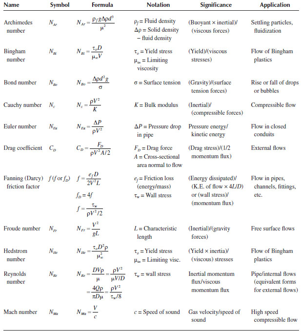
Table 2.2 lists some dimensionless groups that are commonly encountered in fluid mechanics problems. The name of the group and its symbol, definition, significance, and most common area of application are given in the table. Wherever feasible, it is desirable to express basic relations (either theoretical or empirical) in dimensionless form, with the variables being dimensionless groups, because this represents the most general way of presenting results and is independent of scale or specific system properties. We shall follow this guideline insofar as is practical in this book.

VII.    ACCURACY AND PRECISION

First of all, we should make a clear distinction between accuracy and precision. Accuracy is a measure of how close a given value is to the “true” value, whereas precision is a measure of the uncertainty in the value or how “reproducible” that value is. For example, if we were to measure the width of a standard piece of paper using a ruler, we might find that it is 21.5 cm, give or take 0.1 cm. The “give or take” (i.e., the uncertainty) value of 0.1 cm is the precision of the measurement, which is determined by how close we are able to reproduce the measurement with the ruler. However, it is possible that when the ruler is compared with a “standard” unit of measure, it is found to be in error by, say, 0.2 cm. Thus, the “accuracy” of the ruler is limited, which contributes to the uncertainty of the measurement. However, we may not know what this limitation is unless we can compare our “instrument” to one that we know to be true. The accuracy of a given value may be difficult to determine, but the precision of a measurement can be determined by evaluating the reproducibility, if multiple repetitions of the measurement are made. Unfortunately, when using values or data provided by others from handbooks, textbooks, journals, etc., we do not usually have access to either the “true” value or information on the reproducibility of the measured values. However, we can make use of both common sense (i.e., reasonable judgment) and convention to estimate the implied precision of a given value. If the value is represented in scientific notation, the number of digits to the right of the decimal indicates the implied precision (the uncertainty being one-half of the digit to the far right of the decimal point). For example, if the distance from Dallas to Houston is stated as being 250 miles and we drive at 60 miles/h, should we say that it would take us 4.166667 (= 250/60) h for the trip? This number implies that we can determine the answer to a precision of 0.0000005 h, which is one part in 10⁷, or less than 2 ms! This is obviously ludicrous, because the mileage value is nowhere near that precise (is it ±1 mile, ±5 miles?—exactly where did we start and end?), nor can we expect to drive at a speed having this degree of precision (e.g., 60 ± 0.000005 mph, or about ±20 μm/s!). It is conventional to assume that the precision of a given number is comparable to the magnitude of one-half of the last digit in that number. That is, we assume that the value of 250 miles implies 250 ± 0.5 miles (or perhaps ±1 mile). However, unless the numbers are given in scientific notation, so that the least significant digit can be associated with the last digit to the right of the decimal place, there will be some uncertainty, in which case common sense (judgment) should prevail.

TABLE 2.2

Dimensionless Groups in Fluid Mechanics

For example, if the diameter of a tank is specified to be 10.32 ft, we could assume that this value has a precision (or uncertainty) of about 0.005 ft (or 0.06 in., or 1.5 mm). However, if the diameter is said to be 10 ft, the number of digits cannot provide an accurate guide to the precision of the number. It is unlikely that a tank of that size would be constructed to the precision of 1.5 mm, so we would probably assume (optimistically!) that the uncertainty is about 0.5 in., or that the measurement is “roughly 10.0 ft” (i.e., assume three significant digits). However, if I say that I have five fingers on my hand this means exactly five, no more, no less (i.e., an “infinite” number of “significant digits”).

In general, the number of decimal digits that are included in reported data, or the precision to which values can be read from graphs or plots, should be consistent with the precision of the data. Therefore, answers calculated from data with limited precision will likewise be limited in precision (computer people have an acronym for this, i.e., “GIGO,” which stands for “garbage in, garbage out”). When the actual precision of data or other information is uncertain, a general “rule of thumb” is to report numbers to no more than three “significant digits.” This corresponds to an uncertainty of somewhere between 0.05% and 0.5% (which is actually greater precision than can be justified by most engineering data). Inclusion of more than three digits in your answer implies a greater precision than this and should be justified. Those who report values with a large number of digits that cannot be justified are usually making the implied statement “I just wrote down the numbers—I really didn’t think about it.” This is most unfortunate, because if these people don’t think about the numbers they write down, how can we be sure that they are thinking about other critical aspects of the problem?

When combining values, each of which has a finite precision or uncertainty, it is important to be able to estimate the corresponding uncertainty of the result. Although there are various “rigorous” ways of doing this, a very simple method that gives good results as long as the relative uncertainty is a small fraction of the value is to use the approximation (which is really just the first term of a Taylor series expansion):

$A{\left(1\pm a\right)}^x\cong A\left(1\pm xa+\cdots \right),$

which is valid for any value of x if a < 0.1 (about). This assumes that the relative uncertainty of each quantity is expressed as a fraction of the given value, for example, the fractional uncertainty in the value A is a or, equivalently, the percentage error in A is 100a.

SUMMARY

The key points covered in this chapter include the following:

•  The concept of dimensions as related to the physical character of a quantity and units as a measure of the magnitude of the dimensions.

•  The distinction between scientific and engineering systems of dimensions (with associated metric and English units in both systems) and the definition of weight as a gravitational force, being integral to the definition of engineering systems of dimensions.

•  A clear understanding of the distinction between mass and force.

•  The concept that all conversion factors are ratios with a net magnitude of unity and zero dimensions.

•  The “fruit salad law” that says that all terms in a given equation must have the same net dimensions (and the same units) if the equation is valid.

•  Numerical values that arise in theoretical expressions are normally dimensionless, but often numbers or parameters in empirical expressions are not dimensionless, or may include conversion factors that are applicable only to specific units.

•  The value of any quantity that is dimensionless is the same regardless of the scale or units used in any similar system.

•  The universality of dimensionless quantities that permits them to be used to scale-up results from a small-scale system to apply to a larger similar system.

•  Replacing the collection of variables (and parameters) that govern a particular system with the appropriate dimensionless groups of these variables results in a fewer number of variables necessary to describe the system, and renders relationships between these variables independent of scale or size of the system.

•  Understanding that dimensional analysis merely replaces the collection of individual variables in a given problem with fewer corresponding dimensionless variables (groups), but does not provide a relation between these variables.

•  Understanding the difference between accuracy and precision and methods for determining each.

PROBLEMS

UNITS AND DIMENSIONS

1.  Determine the weight of 1 g mass at sea level in units of:

(a)  dynes

(b)  lb_f

(c)  g_f

(d)  poundals

2.  One cubic foot of water weighs 62.4 lb_f under conditions of standard gravity.

(a)  What is its weight in dynes, poundals, and g_f?

(b)  What is its density in lb_m/ft³ and slugs/ft³?

(c)  What is its weight on the moon (g = 5.4 ft/s²) in lb_f?

(d)  What is its density on the moon?

3.  The acceleration due to gravity on the moon is about 5.4 ft/s². If your weight is 150 lb_f on the earth:

(a)  What is your mass on the moon, in slugs?

(b)  What is your weight on the moon, in SI units?

(c)  What is your weight on earth, in poundals?

4.  You weigh a body with a mass m on an electronic scale, which is calibrated with a known mass.

(a)  What does the scale actually measure, and what are its dimensions?

(b)  If the scale is calibrated in the appropriate system of units, what would the scale reading be if the mass of m is (1) 1 slug; (2) 1 lb_m (in scientific units); (3) 1 lb_m (in engineering units); (3) 1 g_m(in scientific units); (4) 1 g_m (in engineering units).

5.  Explain why the gravitational “constant” (g) is different at Reykjavik, Iceland, than it is at Quito, Ecuador. At which location is it greatest, and why? If you could measure the value of g at these two locations, what would this tell you about the earth?

6.  You have purchased a 5 oz bar of gold (100% pure), at a cost of $400/oz. Because the bar was weighed in air, you conclude that you got a bargain, because its true mass is greater than 5 oz due to the buoyancy of air. If the true density of the gold is 1.9000 g/cm³, what is the actual value of the bar based upon its true mass?

7.  You purchased 5 oz of gold in Quito, Ecuador (g = 977.110 cm/s²), for $400/oz. You then took the gold and the same spring scale on which you weighed it in Quito to Reykjavik, Iceland (g = 983.06 cm/s²), where you weighed it again and sold it for $400/oz. How much money did you make or lose, or did you break even?

8.  Calculate the pressure at a depth of 2 miles below the surface of the ocean. Explain and justify any assumptions you make. The physical principle that applies to this problem can be described by the equation

$\Phi =\text{constant},$

where

Φ = P+ρgz

z is the vertical distance measured upward from any horizontal reference plane

Express your answer in units of (a) atm, (b) psi, (c) Pa, (d) poundal/ft², (e) dyn/cm², (f) kg_f/m², (g) N/m².

9.  (a)  Use the principle in Problem 8 to calculate the pressure at a depth of 1000 ft below the surface of the ocean (in psi, Pa, and atm). Assume that the ocean water density is 64 lb_m/ft³.

(b)  If this ocean were on the moon, what would be the answer to (a)? Use the following information to solve this problem: The diameter of the moon is 2160 miles, the diameter of the earth is 8000 miles, and the density of the earth is 1.6 times that of the moon.

10.  The following formula for the pressure drop through a valve was found in a design manual:

$h_L=\frac{522K{q}^2}{d^4},$

where

h_L is the “head loss” in feet of fluid flowing through the valve

K is the dimensionless resistance coefficient for the valve

q is the flow rate through the valve, in ft³/s

d is the diameter of the valve, in in.

(a)  Can this equation be used without changing anything if SI units are used for the variables? Explain.

(b)  What are the dimensions of “522” in this equation? What are its units?

(c)  Determine the pressure drop through a 2 in. valve with a K of 4 for water at 20°C flowing at a rate of 50 gpm, in units of: (1) feet of water, (2) psi, (3) atm, (4) Pa, (5) dyn/cm²; and (6) inches of mercury.

11.  When the energy balance on the fluid in a stream tube is written in the following form, it is known as the Bernoulli equation:

$\frac{P_2-P_1}{\rho }+g\left(z_2-z_1\right)+\frac{\alpha }{2}\left(V_2^2-V_1^2\right)+e_f+w=0,$

where

w is the work done on a unit mass of fluid

e_f is the energy per unit mass dissipated by friction in the fluid, including all thermal energy effects due to heat transfer or internal generation

α is equal to either 1 or 2 for turbulent or laminar flow, respectively

If P₁ = 25 psig, P₂ = 10 psig, z₁ = 5 m, z₂ = 8 m, V₁ = 20 ft/s, V₂ = 5 ft/s, ρ = 62.4 lb_m/ft³, α = 1, and w = 0, calculate the value of e_f in each of the following systems of units:

(a)  SI

(b)  mks engineering (e.g., metric engineering)

(c)  English engineering

(d)  English scientific (with M as a fundamental dimension)

(e)  English thermal units (e.g., Btu)

(f)  Metric thermal units (e.g., calories)

CONVERSION FACTORS, PRECISION

12.  Determine the value of the gas constant, R, in units of ft³ atm/lb mol °R), starting with the value of the standard molar volume of a perfect gas (i.e., 22.4 m³/kg mol).

13.  Calculate the value of the Reynolds number for sodium flowing at a rate of 50 gpm through a tube with a 1/2 in. ID, at 400°F.

14.  The conditions at two different positions along a pipeline (at points 1 and 2) are related by the Bernoulli equation (see Problem 11). For flow in a pipe,

$e_f=\left(\frac{4fL}{D}\right)\left(\frac{V^2}{2}\right),$

where

D is the pipe diameter

L is the pipe length between points 1 and 2

If the flow is laminar (N_Re < 2000), the value of α = 2 and f = 16/N_Re, but for turbulent flow in a smooth pipe, α = 1 and $f=0.0791/N_{Re}^{1/4}$. The work done by a pump on the fluid (−w) is related to the power delivered to the fluid (HP) and the mass flow rate of the fluid (ṁ) by HP = −wṁ. Consider water (ρ = 1 g/cc, μ = 1 cP) being pumped at a rate of 150 gpm through a 2000 ft long 3 in. diameter pipe. The water is transported from a reservoir (z = 0) at atmospheric pressure to a condenser at the top of a column that is at an elevation of 30 ft and a pressure of 5 psig. Determine

(a)  The value of the Reynolds number in the pipe

(b)  The value of the friction factor in the pipe (assuming that it is smooth)

(c)  The power that the pump must deliver to the water, in horsepower (hp)

15.  The Peclet number (N_Pe) is defined as

$N_{Pe}=N_{Re}{N}_{Pr}=\left(\frac{DV\text{ρ}}{\text{μ}}\right)\left(\frac{c_p\text{μ}}{k}\right)=\frac{DG{c}_p}{\text{μ}},$

where

D is the pipe diameter

G is the mass flux = ρV

c_p is the specific heat

k is the thermal conductivity

μ is the viscosity

Calculate the value of N_Pe for water at 60°F flowing through a 1 cm. diameter tube at a rate of 100 lb_m/h. (Use the most accurate data you can find, and state your answer in the appropriate number of digits consistent with the data you use.)

16.  The heat transfer coefficient (h) for a vapor bubble rising through a boiling liquid is given by

$h=A{\left(\frac{kV\text{ρ}{c}_p}{d}\right)}^{1/2}\text{where}V=\left(\frac{\Delta \text{ρ}g\sigma }{{\text{ρ}}_{\text{v}}^2}\right),$

where

h is the heat transfer coefficient [e.g., Btu/(h °F ft²)]

c_p is the liquid heat capacity [e.g., cal/(g °C)]

k is the liquid thermal conductivity [e.g., J/(s K m)]

σ is the liquid/vapor surface tension [e.g., dyn/cm]

Δρ= ρ_liquid − ρ_vapor = ρ_l − ρ_v,

d is the bubble diameter

g is the acceleration due to gravity

(a)  What are the fundamental dimensions of V and A?

(b)  If the value of h is 1000 Btu/(h ft²°F) for a 5 mm diameter steam bubble rising in boiling water at atmospheric pressure, determine the corresponding values of V and A in SI units. You must look up values for the other quantities you need, and be sure to cite the sources you use for these data.

17.  Determine the value of the Reynolds number for SAE 10 lube oil at 100°F flowing at a rate of 2000 gpm through a 10 in. Schedule 40 pipe. The oil SG is 0.92, and its viscosity can be found in Appendix A. If the pipe is made of commercial steel (ε = 0.0018 in.), use the Moody diagram (see Figure 6.4) to determine the friction factor f for this system. Estimate the precision of your answer, based upon the information and procedure you use to determine it (i.e., tell what the reasonable upper and lower bounds, or the corresponding percentage variation, should be for the value of f based on the information you used).

18.  Determine the value of the Reynolds number for water flowing at a rate of 0.5 gpm through a 1 in. ID pipe. If the diameter of the pipe is doubled at the same flow rate, how much will each of the following change:

(a)  The Reynolds number

(b)  The pressure drop

(c)  The friction factor

19.  The pressure drop for a fluid with a viscosity of 5 cP and a density of 0.8 g/cm³ flowing at a rate of 30 g/s in a 50 ft long 1/4 in. diameter pipe is 10 psi. Use this information to determine the pressure drop for water at 60°F flowing at 0.5 gpm in a 2 in. diameter pipe. What is the value of the Reynolds number for each of these cases?

DIMENSIONAL ANALYSIS AND SCALE-UP

20.  In the steady flow of a Newtonian fluid through a long uniform circular tube, if N_Re < 2000, the flow is laminar and the fluid elements move in smooth straight parallel lines. Under these conditions, it is known that the relationship between the flow rate and the pressure drop in the pipe does not depend upon the fluid density or the pipe wall material.

(a)  Perform a dimensional analysis of this system to determine the dimensionless groups that apply. Express your result in a form in which the Reynolds number can be identified.

(b)  If water is flowing at a rate of 0.5 gpm through a pipe with an ID of 1 in., what is the value of the Reynolds number? If the diameter is doubled at the same flow rate, what will be the effect on the Reynolds number and on the pressure drop?

21.  Perform a dimensional analysis to determine the groups relating the variables that are important in determining the settling rate of very small solid particles falling in a liquid. Note that the driving force for moving the particles is gravity and the corresponding net weight of the particle. At very slow settling velocities, it is known that the velocity is independent of the fluid density. Show that this also requires that the velocity be inversely proportional to the fluid viscosity.

22.  A simple pendulum consists of a small, heavy ball of mass m at the end of a long string of length L. The period of the pendulum should depend on these factors, as well as gravity, which is the driving force for making it move. What information can you get about the relationship between these variables from a consideration of their dimensions? Suppose you measured the period, T₁ of a pendulum with mass m₁ and length l₁. How could you use this to determine the period of a different pendulum with a different mass and length? What would be the ratio of the pendulum period on the moon to that on the earth? How could you use the pendulum to determine the variation of g on the earth’s surface?

23.  An ethylene storage tank in your plant explodes. The distance that the blast wave travels from the blast site (R) depends upon the energy released in the blast (E), the density of the air (ρ), and time (t). Use dimensional analysis to determine:

(a)  The dimensionless group(s) that can be used to describe the relationship between the variables in the problem;

(b)  The ratio of the velocity of the blast wave at a distance of 2000 ft from the blast site to the velocity at a distance of 500 ft from the sites;

The pressure difference across the blast wave (ΔP) also depends upon the blast energy (E), the air density (ρ), and time (t). Use this information to determine:

(c)  The ratio of the blast pressure at a distance of 500 ft from the blast site to that at a distance of 2000 ft from the site.

24.  It is known that the power required to drive a fan depends upon the impeller diameter (D), the impeller rotational speed (ω), the fluid density (ρ), and the volume flow rate (Q). (Note that the fluid viscosity is not important for gases under normal conditions.)

(a)  What is the minimum number of fundamental dimensions required to define all of these variables?

(b)  How many dimensionless groups are required to determine the relationship between the power and all the other variables? Find these groups by dimensional analysis, and arrange the results so that the power and the flow rate each appear in only one group.

25.  A centrifugal pump with an 8 in. diameter impeller operating at a rotational speed of 1150 rpm requires 1.5 hp to deliver water at a rate of 100 gpm and a pressure of 15 psi. Another pump for water, which is geometrically similar but has an impeller diameter of 13 in., operates at a speed of 1750 rpm. Estimate the pump pressure, flow capacity, and power requirements of this second pump. (Under these conditions, the performance of both pumps is independent of the fluid viscosity.)

26.  A gas bubble of diameter D rises with a velocity V in a liquid of density ρ and viscosity μ.

(a)  Determine the dimensionless groups that include the effects of all of the significant variables, in such a form that the liquid viscosity appears in only one group. Note that the driving force for the bubble motion is buoyancy, which is equal to the weight of the displaced fluid.

(b)  You want to know how fast a 5 mm diameter air bubble will rise in a liquid with a viscosity of 20 cP and a density of 0.85 g/cm³. You want to simulate this system in the laboratory using water (μ = 1 cP, ρ = 1 g/cm³) and air bubbles. What size (diameter) air bubble should you use?

(c)  You perform the experiment, and measure the velocity of the air bubble in water (V_m). What is the ratio of the velocity of the 5 mm diameter bubble in the field liquid (V_f) to that in the lab (V_m)?

27.  You must predict the performance of a large industrial mixer under various operating conditions. To obtain the necessary data, you decide to run a laboratory test on a small-scale model of the unit. You have deduced that the power (P) required to operate the mixer depends upon the following variables:

Tank diameter, D

Impeller diameter, d

Impeller rotational speed,N

Fluid density, ρ

Fluid viscosity, μ

(a)  Determine the minimum number of fundamental dimensions involved in these variables and the number of dimensionless groups that can be defined by them.

(b)  Find an appropriate set of dimensionless groups such that D and N each appear in only one group. If possible, identify one or more of the groups with groups commonly encountered in other systems.

(c)  You want to know how much power would be required to run a mixer in a large tank 6 ft in diameter, using an impeller with a diameter of 3 ft operating at a speed of 10 rpm, when the tank contains a fluid with a viscosity of 25 cP and a specific gravity of 0.85. To do this, you run a lab test on a model of the system, using a scale model of the impeller that is 10 in. in diameter. The only appropriate fluid you have in the lab has a viscosity of 15 cp and a specific gravity of 0.75. Can this fluid be used for the test? Explain.

(d)  If the preceding lab fluid is used, what size of the tank should be used in the lab, and how fast should the lab impeller be rotated?

(e)  With the lab test properly designed and the proper operating conditions chosen, you run the test and find that it takes 150 W to operate the lab test model. How much power would be required to operate the larger field mixer under the plant operating conditions?

28.  When an open tank with a free surface is stirred with an impeller, a vortex will form around the shaft. It is important to prevent this vortex from reaching the impeller, because entrainment of air in the liquid tends to cause foaming. The shape of the free surface depends upon (among other things) the fluid properties, the speed and size of the impeller, the size of the tank, and the depth of the impeller below the free surface.

(a)  Perform a dimensional analysis of this system to determine an appropriate set of dimensionless groups that can be used to describe the system performance. Arrange the groups so that the impeller speed appears in only one group.

(b)  In your plant you have a 10 ft diameter tank containing a liquid that is 8 ft deep. The tank is stirred by an impeller that is 6 ft in diameter and is located 1 ft from the tank bottom. The liquid has a viscosity of 100 cP and a specific gravity of 1.5. You need to know the maximum speed at which the impeller can be rotated without entraining the vortex in the impeller blades. To find this out, you design a laboratory test using a scale model of the impeller that is 8 in. in diameter. What, if any, limitations are there on your freedom to select a fluid for use in the lab test?

(c)  Select an appropriate fluid for the lab test and determine how large the tank used in the lab should be and where in the tank the impeller should be located.

(d)  The lab impeller is run at such a speed that the vortex just reaches the impeller. What is the relation between this speed and that at which entrainment would occur in the tank in the plant?

29.  The variables involved in the performance of a centrifugal pump include the fluid properties (μ and ρ), the impeller diameter (d), the casing diameter (D), the impeller rotational speed (N), the volumetric flow rate of the fluid (Q), the head (H) developed by the pump (ΔP = ρgH), and the power required to drive the pump (HP).

(a)  Perform a dimensional analysis of this system to determine an appropriate set of dimensionless groups that would be appropriate to characterize the pump. Arrange the groups so that the fluid viscosity and the pump power each appear in only one group.

(b)  You want to know what pressure a pump will develop with a liquid that has a specific gravity of 1.4 and a viscosity of 10 cP, at a flow rate of 300 gpm. The pump has an impeller with a diameter of 12 in., which is driven by a motor running at 1100 rpm. (It is known that the pump performance is independent of fluid viscosity unless the viscosity is greater than about 50 cP.) You want to run a lab test that simulates the operation of the larger field pump using a similar (scaled) pump with an impeller that has a diameter of 6 in. and a 3600 rpm motor. Should you use the same liquid in the lab as in the field, or can you use a different liquid? Why?

(c)  If you use the same liquid, what flow rate should be used in the lab to simulate the operating conditions of the field pump?

(d)  If the lab pump develops a pressure of 150 psi at the proper flow rate, what pressure will the field pump develop with the field fluid?

(e)  What pressure would the field pump develop with water at a flow rate of 300 gpm?

30.  The purpose of a centrifugal pump is to increase the pressure of a liquid in order to move it through a piping system. The pump is driven by a motor, which must provide sufficient power to operate the pump at the desired conditions. You wish to find the pressure developed by a pump operating at a flow rate of 300 gpm with an oil having a specific gravity (SG) of 0.8 and a viscosity of 20 cP, and the required horsepower for the motor to drive the pump. The pump has an impeller diameter of 10 in., and the motor runs at 1200 rpm.

(a)  Determine the dimensionless groups that would be needed to completely describe the performance of the pump.

(b)  You want to determine the pump pressure and motor horsepower by measuring these quantities in the lab on a smaller-scale model of the pump that has a 3 in. diameter impeller and a 1800 rpm motor, using water as the test fluid. Under the operating conditions for both the lab model and the field pump, the value of the Reynolds number is very high, and it is known that the pump performance is independent of the fluid viscosity under these conditions. Determine the proper flow rate at which the lab pump should be tested and the ratio of the pressure developed by the field pump to that of the lab pump operating at this flow rate as well as the ratio of the required motor power in the field to that in the lab.

(c)  The pump efficiency (η_e) is the ratio of the power delivered by the pump to the fluid (as determined by the pump pressure and flow rate) to the power delivered to the pump by the motor. Because this is a dimensionless number, it should also have the same value for both the lab and field pumps when they are operating under equivalent conditions. Is this condition satisfied?

31.  When a ship moves through the water, it causes waves. The energy and momentum in these waves must come from the ship, which is manifested as a “wave drag” force on the ship. It is known that this drag force (F) depends upon the ship speed (V), the fluid properties (ρ, μ), the length of the waterline (L), and the beam width (W) as well as the shape of the hull, among other things. (There is at least one important “other thing” that relates to the “wave drag,” i.e., the energy required to create and sustain the waves from the bow and the wake. What is this additional variable?) Note that “shape” is a dimensionless parameter, which is implied by the requirement of geometrical similarity. If two geometries have the same shape, the ratio of each corresponding dimension of the two will also be the same.

(a)  Perform a dimensional analysis of this system to determine a suitable set of dimensionless groups that could be used to describe the relationship between all of the variables. Arrange the groups such that viscous and gravitational parameters each appear in separate groups.

(b)  It is assumed that “wave drag” is independent of viscosity and that “hull drag” is independent of gravity. You wish to determine the drag on a ship having a 500 ft long waterline moving at 30 mph through seawater (SG = 1.1). You can make measurements on a scale model of the ship, 3 ft long, in a towing tank containing fresh water. What speed should be used for the model to simulate the wave drag and the hull drag?

32.  You want to find the force exerted on an undersea pipeline by a 10 mph current flowing normal to the axis of the pipe. The pipe is 30 in. in diameter, and the density of seawater is 64 lb_m/ft³ and its viscosity is 1.5 cP. To determine this, you test a 1½ in. diameter model of the pipe in a wind tunnel at 60°F. What velocity should you use in the wind tunnel in order to scale the measured force to the conditions in the sea? What is the ratio of the force on the pipeline in the sea to that on the model measured in the wind tunnel?

33.  You want to determine the thickness of the film when a Newtonian fluid flows uniformly down an inclined plane at an angle θ with the horizontal at a specified flow rate. To do this, you design a laboratory experiment from which you can scale up measured values to any other Newtonian fluid under corresponding conditions.

(a)  List all the independent variables that are important in this problem, with their dimensions. If there are any variables that are not independent but act only in conjunction with one another, list only the net combination that is important.

(b)  Determine an appropriate set of dimensionless groups for this system, in such a way that the fluid viscosity and the plate inclination each appear in only one group.

(c)  Decide what variables you would choose for convenience, what variables would be specified by the analysis, and what you would measure in the lab.

34.  You would like to know the thickness of a syrup film as it drains at a rate of 1 gpm down a flat surface that is 6 in. wide and is inclined at an angle of 30° from the vertical. The syrup has a viscosity of 100 cP and a SG of 0.9. In the laboratory, you have a fluid with a viscosity of 70 cP and a SG of 1.0 and a 1 ft wide plane inclined at an angle of 45° from the vertical.

(a)  At what flow rate, in gpm, would the laboratory conditions simulate the specified conditions?

(b)  If the thickness of the film in the laboratory is 3 mm at the proper flow rate, what would the thickness of the film be for the 100 cP fluid at the specified conditions?

35.  The size of liquid droplets produced by a spray nozzle depends upon the nozzle diameter, the fluid velocity, and the fluid properties (which may, under some circumstances, include surface tension).

(a)  Determine an appropriate set of dimensionless groups for this system.

(b)  You want to know what size droplets will be generated by a fuel oil nozzle with a diameter of 0.5 mm at an oil velocity of 10 m/s. The oil has a viscosity of 10 cP, a SG of 0.82, and a surface tension of 35 dyn/cm. You have a nozzle in the lab with a nozzle diameter of 0.2 mm that you want to use in a lab experiment to find the answer. Can you use the same fuel oil in the lab test as in the field? If not, why not?

(c)  If the only fluid you have is water, tell how you would design the lab experiment. Note: water has a viscosity of 1 cP and a SG of 1, but its surface tension can be varied by adding small amounts of surfactant that does not affect the viscosity or density.

(d)  Determine what conditions you would use in the lab, what you would measure, and the relationship between the measured and unknown droplet diameters.

36.  Small solid particles of diameter d and density ρ_s are carried horizontally by an air stream moving at velocity V. The particles are initially at a distance h above the ground, and you want to know how far they will be carried horizontally before they settle to the ground. To find this out, you decide to conduct a lab experiment using water as the test fluid.

(a)  Determine what variables you must set in the lab and how the value of each of these variables is related to the corresponding variable in the air system. You should note that several forces act on the particle: the drag force due to the moving fluid, which depends on the fluid and solid properties, the size of the particle and the relative velocity, and the gravitational force, which is directly related to the densities of both the solid and the fluid in a known manner.

(b)  Is there any reason why this experiment might not be feasible in practice?

37.  You want to find the wind drag on a new automobile design at various speeds. To do this, you test a 1/30 scale model of the car in the lab. You must design an experiment whereby the drag force measured in the lab can be scaled up directly to find the force on the full-scale car at a given speed.

(a)  What is the minimum number of (dimensionless) variables required to completely define the relationship between all the important variables in the problem? Determine the appropriate variables (e.g., the dimensionless groups).

(b)  The only fluids you have available in the lab are air and water. Could you use either one of these, if you wanted to? Why (or why not)?

(c)  Tell which of these fluids you would use in the lab, and then determine what the velocity of this fluid past the model car would have to be so that the experiment would simulate the drag on the full-scale car at 40 mph. If you decide that it is possible to use either one of the two fluids, determine the answer for each of them.

(d)  What is the relationship between the measured drag force on the model and the drag force on the full-scale car? If possible, determine this relationship for the other fluid, as well. Repeat this for a speed of 70 mph.

(e)  It turns out that for very high values of the Reynolds number, the drag force is independent of the fluid viscosity. Under these conditions, if the speed of the car doubles, by what factor does the power required to overcome wind drag change?

38.  The power required to drive a centrifugal pump and the pressure that the pump will develop depends upon the size (diameter) and speed (angular velocity) of the impeller, the volumetric flow rate through the pump, and the fluid properties. However, if the fluid is not too viscous (e.g., less than about 100 cP), the pump performance is essentially independent of the fluid viscosity. Under these conditions:

(a)  Perform a dimensional analysis to determine the dimensionless groups that would be required to define the pump performance. Arrange the groups so that the power and pump pressure each appear in only one group.

You have a pump with an 8 in. diameter impeller that develops a pressure of 15 psi and requires 1.5 hp to operate when running at 1150 rpm with water at a flow rate of 100 gpm. You also have a similar pump with a 13 in. diameter impeller, driven by a 1750 rpm motor, and you would like to know what pressure this pump would develop with water and what power would be required to drive it.

(b)  If the second pump is to be operated under equivalent (similar) conditions to the first one, what should the flow rate be?

(c)  If this pump is operated at the proper flow rate, what pressure will it develop, and what power will be required to drive it when pumping water?

39.  In a distillation column, vapor is bubbled through the liquid to provide good contact between the two phases. The bubbles are formed when the vapor passes upward through a hole (orifice) in a plate (tray) that is in contact with the liquid. The size of the bubbles depends upon the diameter of the orifice, the velocity of the vapor through the orifice, the viscosity and density of the liquid, and the surface tension between the vapor and the liquid.

(a)  Determine the dimensionless groups required to completely describe this system, in such a manner that the bubble diameter and the surface tension do not appear in the same group.

(b)  You want to find out what size bubbles would be formed by a hydrocarbon vapor passing through a 1/4 in. orifice at a velocity of 2 ft/s, in contact with a liquid having a viscosity of 4 cP and a density of 0.95 g/cm³ (the surface tension is 30 dyn/cm). To do this, you run a lab experiment using air and water (with a surface tension of 60 dyn/cm).

(i)  What size orifice should you use, and what should the air velocity through the orifice be?

(ii)  You design and run this experiment and find that the air bubbles are 0.1 in. in diameter. What size would the vapor bubbles be in the organic fluid above the 1/4 in. orifice?

40.  A flag will flutter in the wind at a frequency that depends upon the wind speed, the air density, the size of the flag (length and width), gravity, and the “area density” of the cloth (i.e., the mass per unit area). You have a very large flag (40 ft long and 30 ft wide) that weighs 240 lb, and you want to find the frequency at which it will flutter in a wind of 20 mph.

(a)  Perform a dimensional analysis to determine an appropriate set of dimensionless groups that could be used to describe this problem.

(b)  To find the flutter frequency you run a test in a wind tunnel (at normal atmospheric temperature and pressure) using a flag made from a cloth that weighs 0.05 lb/ft². Determine (1) the size of the flag and the wind speed that you should use in the wind tunnel and (2) the ratio of the flutter frequency of the big flag to that which you observe for the model flag in the wind tunnel.

41.  If the viscosity of the liquid is not too high (e.g., less than about 100 cP), the performance of many centrifugal pumps is not very sensitive to the fluid viscosity. You have a pump with an 8 in. diameter impeller that develops a pressure of 15 psi and consumes 1.5 hp when running at 1150 rpm pumping water at a rate of 100 gpm. You also have a similar pump with a 13 in. diameter impeller, driven by a 1750 rpm motor, and you would like to know what pressure that pump would develop with water, and how much power it would take to drive it.

(a)  If the second pump is to be operated under conditions similar to that of the first, what should the flow rate be?

(b)  When operated at this flow rate with water, what pressure should it develop and what power would be required to drive it?

42.  The pressure developed by a centrifugal pump depends on the fluid density, the diameter of the pump impeller, the rotational speed of the impeller, and the volumetric flow rate through the pump (centrifugal pumps are not recommended for highly viscous fluids, so viscosity is not commonly an important variable). Furthermore, the pressure developed by the pump is commonly expressed as the “pump head,” which is the height of a column of the fluid in the pump that exerts the same pressure as the pump pressure.

(a)  Perform a dimensional analysis to determine the minimum number of variables required to represent the pump performance characteristic in the most general (dimensionless) form.

(b)  The power delivered to the fluid by the pump is also important. Should this be included in the list of important variables, or can it be determined from the original set of variables? Explain.

You have a pump in the field that has a 1.5 ft diameter impeller that is driven by a motor operating at 750 rpm. You want to determine what head the pump will develop when pumping a liquid with density of 50 lb_m/ft³ at a rate of 1000 gpm. You do this by running a test in the lab on a scale model of the pump that has a 0.5 ft diameter impeller using water (at 70°F) and a motor that runs at 1200 rpm.

(c)  At what flow rate of water should the lab pump be operated (in gpm)?

(d)  If the lab pump develops a head of 85 ft at this flow rate, what head would the pump in the field develop with the operating fluid at the specified flow rate?

(e)  How much power (in horsepower) is transferred to the fluid in both the lab and the field cases?

(f)  The pump efficiency is defined as the ratio of the power delivered to the fluid to the power of the motor that drives the pump. If the lab pump is driven by a 2 hp motor, what is the efficiency of the lab pump? If the efficiency of the field pump is the same as that of the lab pump, what power motor (horsepower) would be required to drive it?

NOTATION

D	Inside pipe diameter, [L]
f	Friction factor, [—]
F	Dimension of force
G	Gravitational constant = 6.67 × 10−11 N m2/kg2, Equation 2.2, [FL2/M2] = [L3/Mt2]
g	Acceleration due to gravity, [L/t2]
gc	Conversion factor, [ML/(Ft2)]
ID	Inside diameter of pipe, [L]
K1	Loss parameter (see Chapter 7), [—]
Kd	Loss parameter (see Chapter 7), [—]
Kf	Loss coefficient (see Chapter 7), [—]
K	Loss parameter (see Chapter 7), [—]
ke	Kinetic energy per unit mass, [FL/M = L2/t2]
L	Dimension of length
L	Length, [L]
M	Dimension of mass
m	Mass, [M]
NRe	Reynolds number, [—]
Nx	Dimensionless group x [—]
P	Pressure, [F/L2 = M/(Lt2)]
Q	Volumetric flow rate, [L3/t]
R	Radius, [L]
T	Torque, [FL = ML2/t2]
t	Dimension of time
t	Time [t]
V	Spatial average velocity, [L/t] v Local velocity, [L/t]
W	Weight, [F = ML/t2]
x	Coordinate direction, [L]
z	Coordinate direction (measured upward), [L]

GREEK

ε	Roughness, [L]
μ	Viscosity, [M/Lt]
ρ	Density, [M/L3]
τyx	Shear stress, force in x direction on y surface, [F/L2 = ML/t2]

SUBSCRIPTS

1	Upstream reference point 1
2	Downstream reference point 2
m	“Model”
f	“Field”
x, y, r, θ	Coordinate directions

*  Although this system of units originated in England, the English have since adopted the SI (metric) system. However, this system is still in use by most companies and the public in the United States and hence is sometimes called the American system.

*  We use the recommended notation of the AIChE for dimensionless groups that are named after their originator, that is, a capital N with a subscript identifying the person the group is named for, such as N_Re for Reynolds number, N_Ar for Archimedes number, etc. However, there are a variety of other dimensionless quantities that are identified by other symbols.

*  English engineering units are often referred to as American engineering units.