
“If I have ever made any valuable discoveries, it has been owing more to patient attention, than to any other talent.”
—Isaac Newton, 1643–1727, Scientist
It is imperative that all pressure vessels be equipped with a relief device to prevent the pressure from exceeding the maximum allowable working pressure (MAWP) of the vessel, with the consequent rupture of the vessel and loss of containment of the contents. A typical installation is illustrated in Figure 11.1. Typical “worst case” scenarios that could result in excessive pressure buildup include runaway reactions, blockage of discharge lines, external fires, etc. A safety relief valve (SRV) is designed to open at a preset “set pressure” and close when the pressure drops below that pressure by a set amount (“blowdown”) in order to minimize the loss of containment. A rupture disk is sometimes used to relieve the vessel pressure, but when it ruptures virtually all of the vessel contents is lost. More detailed discussion of the selection, design, and operation of safety relief and control valves can be found in several books, e.g., CCPS, AIChE (1998), Cheremisinoff and Cheremisinoff (1987), Liptak (2006), etc.
The design of a relief system begins with an energy balance on the system (i.e., the fluid in the vessel) to determine the rate of energy input from the source (e.g., a runaway reaction, blocked line, external fire, etc.). Then the relief valve must be sized so that the mass flow rate through the valve releases this energy at a rate which is equal to or greater than it is input to the vessel from the source, at the desired pressure. The valve relief pressure is normally set at 10% above the MAWP (Maximum Allowed Working Pressure) of the vessel (depending on the energy source), and the valve must be sized for the required mass flow at this pressure. Thus, it is assumed that this determination of the required mass flow rate has been done prior to calculating the required valve size.
A typical spring-loaded pop action SRV is shown in Figure 11.2a. The spring determines the pressure at which the valve opens and the disk lifts. The relieving fluid flows through the nozzle and out of the valve through discharge piping. The nozzle provides the smallest flow area and thus controls the flow rate.
The determination of the proper size of the relief valve (nozzle or orifice) required to properly discharge the contents of a pressure vessel at a mass flow rate sufficient to prevent excessive pressure buildup in the vessel requires the following three types of information:
• A model for the flow configuration in the valve (the flow model).
• A model for the properties of the fluid in the valve (a fluid property model).
• Data for the flow capacity of the actual valve with the type of fluid of interest (valve flow data, i.e. the valve discharge coefficient).
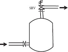
FIGURE 11.1 Typical safety relief valve installation.
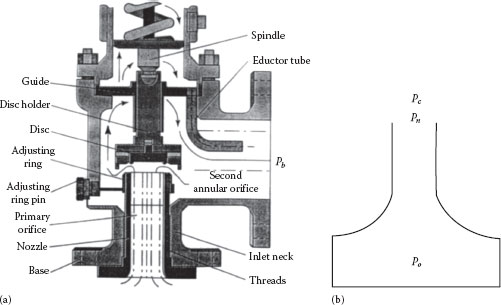
FIGURE 11.2 (a) A typical spring-loaded safety valve and (b) ideal nozzle geometry. (a: Courtesy of Consolidated Valve Co.)
The reference geometrical configuration for the flow model for relief valve flow analysis is the isentropic nozzle, an idealized representation of which is shown in Figure 11.2b.
The basic equation for the mass flux through an isentropic nozzle follows directly from the frictionless differential Bernoulli equation:
(11.1) |
Integration of this equation for the velocity u from the stagnation state in the vessel (P = Po, u = 0) to the nozzle exit (Pn), and expressing the result in terms of the mass flux through the nozzle, Go = ρu = ṁ/A, gives
(11.2) |
Once the mass flux is known, the nozzle or “orifice” area is determined from the known mass flow rate, that is, A = ṁ/G. If this area falls between two standard-size available orifices, the larger of the two is selected. The frictional pressure drop in the entrance line from the vessel to the valve is limited by the API recommendations to 3% of the valve set pressure or less, so if this is satisfied this pressure drop is commonly neglected in practice.
For adiabatic flow, Equation 11.1 can also be written as
(11.3) |
Integrating this expression across the nozzle gives
(11.4) |
where H is the specific enthalpy (per unit mass) of the fluid. Equation 11.4 is more general than Equation 11.2 in that Equation 11.4 is not restricted to isentropic processes as is the case for Equation 11.2. However, the mass flux calculated by Equation 11.4 is very sensitive to slight variations in the values of the enthalpy (because of the large conversion factor from thermal to mechanical energy units (e.g., 778 ft lbf/Btu). This requires highly accurate enthalpy values for determining reliable mass flux values. Such accuracy is not widely available, so that Equation 11.2 is preferred in general.
The fluid property model is the relation between the fluid density (single- or two-phase) and pressure, that is, ρ(P), which is necessary to evaluate the integral in Equation 11.2. This can be the actual measured or calculated density or values estimated from an appropriate equation of state (EOS). As with any thermodynamic property, the density is a function of two independent parameters such as ρ(P, S) or ρ(P, H) or ρ(P, T). For an ideal nozzle, the fluid follows an isentropic path so the density should be expressed simply as ρ(P)S, or density as a function of pressure at constant entropy. In some simple cases, such as the flow of an incompressible fluid or the flow of an ideal gas, the density can be determined accurately. In more complex systems, such as two-phase flashing flow, the density versus pressure may be determined from data or an EOS model and tabulated in a thermodynamic property database (e.g. steam tables, NIST (2015), etc.).
The valve flow data are represented by a discharge coefficient, defined as
(11.5) |
where
Gn is the measured mass flux for a test fluid through a representative valve of a particular type, for a specific fluid, under specific conditions
Go is the theoretically predicted mass flux from the isentropic nozzle and fluid property models
Thus, the value of KD accounts for any discrepancies between the isentropic nozzle and fluid property models, and the flow in the actual valve. It is therefore a correction factor that multiplies the theoretical isentropic model mass flux to give the actual mass flux. If the fluid property model is accurate, KD should be a function only of the valve geometry and flow conditions (e.g., turbulence level, choking, etc., similar to the dependence of the pipe friction factor or fitting loss coefficients on geometry and turbulence level) and independent of fluid properties. It sometimes happens that a reference fluid is used to calculate the mass flux, in which case the discharge coefficient must also reflect the difference between the properties of the reference fluid and the actual fluid. For a given valve, the values of KD for gas flows (KDG) and for liquid flows (KDL) are significantly different, which will be explained later.
There are exact solutions for the mass flux for liquids and ideal gases, as shown below. There are also many “models” for nonideal and two-phase fluids, all of which assume that the fluid is homogeneous, that is, each of the two phases is highly turbulent and sufficiently well mixed that they can be described as a “pseudo-single-phase” fluid, with a suitable average density. The following gives the most significant of these results (according to the judgment of the authors).
It is emphasized that Go in the following equations is the theoretical calculated value for the isentropic nozzle and must be corrected by applying the empirical KD (e.g., KDL for liquids or KDG for gases). The significance of KD is discussed later.
Most liquids under ordinary conditions can be considered “incompressible” or isochoric, with a constant density. For these fluids, evaluation of the integral in Equation 11.2 is direct and gives
(11.6) |
As the pressure at the nozzle (Pn) is not normally known, it is assumed to be the same as that at the exit of the valve, or the “backpressure,” under the assumption that the pressure drop in the valve body is negligible (more on this later). The above equation assumes fully turbulent flow (high Reynolds number), where the effect of the fluid viscosity is negligible.
If the fluid is sufficiently viscous that the Reynolds number through the nozzle is about 10,000 or less, a viscosity “correction factor,” Kv, is required. A curve for this correction factor is presented in API 520-1, which was actually adapted from a study by Stiles (1964) on control valves. More recently, Darby and Molavi (1997) presented a CFD (Computational Fluid Dynamics) solution for a viscous fluid in a typical valve geometry to determine the viscosity correction factor. The results are shown in Figure 11.3, along with the API curve.
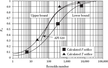
FIGURE 11.3 Viscosity correction factor. (From Darby and Molavi, 1997.)
The equation that represents the curves shown on the plot is
(11.7) |
where β = Dn/Dp is the ratio of the nozzle diameter to the inlet pipe diameter, and the Reynolds number is based on the nozzle throat diameter.
The calculations were performed for two orifice sizes, F and T, with β values of 0.422 and 0.757, respectively.
Many gases can be described by the ideal gas law, that is, ρ = PM/RT, over a fairly wide range of conditions, which under isentropic conditions is P/ρk = constant, where k is the “isentropic exponent” (for an ideal gas, k = γ is the specific heat ratio, cp/cv). This model is quite accurate for most gases sufficiently far removed from the thermodynamic critical point (such as air or nitrogen under reasonable conditions). The value of k for air under standard conditions is about 1.4, and it varies only slightly with temperature and pressure. These relations can be used to evaluate the integral in Equation 11.2 to give
(11.8) |
It can be seen from this equation that as the nozzle pressure, Pn, decreases, the mass flux increases until it reaches a maximum value at
(11.9) |
At this point, the flow is choked and is independent of the nozzle downstream pressure (Pn). If no maximum is reached before Pn drops to the valve exit pressure, then the flow is not choked. The criterion for choked flow is
(11.10) |
For real gases (pure or mixtures), k is a function of pressure as well as temperature and may be evaluated from an appropriate EOS, or from a thermodynamic database as described below for two-phase flows. For a nonideal gas, it is often adequate to use Equations 11.9 and 11.10, with an average value of k over the range of T, P of interest.
Example 11.1
A relief valve must be selected to discharge a vessel at a rate of 75 lbm/s when fully open from a vessel for which the maximum allowed pressure is 150 psia. The fluid is a vapor with a molecular weight of 45, which can be considered an ideal gas, with a specific heat ratio of 1.3, a temperature of 70°F, and it is discharged into the atmosphere. Determine the diameter of the nozzle in the valve that should be selected (Note: if the calculated nozzle area does not match any of the standard sizes available, the next larger size is selected. An additional 10% is also usually added to the calculated nozzle area as a “safety factor.”)
Solution:
For an ideal gas, the theoretical expression Equation 11.8 applies:
The expression for the exit pressure at which the flow is choked is given by Equation 11.10:
Thus, because Pc > Pb, the flow is choked and Pn = 81.86 psia. Thus, Equation 11.9 applies:
Assume KG = 0.975, and applying the 10% safety factor:
3. The Homogeneous Direct Integration Method for Any Single- or Two-Phase Flow
There are a large number of “models” for two-phase flows, both “frozen” and “flashing,” for which the two phases are assumed to be in thermodynamic equilibrium. “Frozen” flows involve nonvolatile liquids and noncondensable gases (e.g., air and water) with constant quality (i.e., mass fraction of gas, x), whereas flashing flows involve a volatile liquid and a change of quality as the liquid flashes. Most of these models require a knowledge of the physical/thermodynamic properties sufficient to evaluate the function ρ = fn(P) for at least one or more conditions (e.g., P, T) within the nozzle. If this information is available, it is easier and much more general and accurate to evaluate this function at a series of points from Po to Pn (or to the choke pressure, Pc) and to use a finite difference procedure to evaluate the integral in Equation 11.2, such as:
(11.11) |
Here, the density as a function of pressure is evaluated over an isentropic path from Po to Pn using an appropriate physical property database. This method is referred to as the homogeneous direct integration (HDI) method (Darby et al., 2002; Darby, 2004).
The mass flux will increase as Pn is decreased until a maximum in Go (i.e., Gc) is reached, at which point the flow is choked and Pn = Pc. If Pn is reached before the mass flux reaches a maximum, then the flow is not choked. The procedure is to first select an appropriate pressure increment (1% of the difference between Po and Pb is usually more than adequate). Then, utilizing the thermodynamic property data for the fluid (or mixture), determine the density of the fluid (single- or two-phase), and hence the mass flux, Go, at successive increments of Pn over a constant entropy path, starting with Pn =Po. As Pn is decreased, Go will increase until it reaches a maximum, at which point the flow is choked at pressure Pc, which is the lowest pressure that can exist inside the nozzle exit. If no maximum is reached before Pn = Pb (the back pressure on the valve), then the flow is not choked. As long as a suitable property database is available (and there are many), this procedure works well for any fluid (single- or two-phase, frozen or flashing, single- or multicomponent, etc.) under equilibrium conditions.
The density of the two-phase mixture is related to the density of each phase and the quality, or mass fraction of the vapor/gas phase, (x), by
(11.12) |
where
(11.13) |
is the volume fraction of vapor/gas in the flowing mixture and S is the “slip factor.” The slip factor is the ratio of the velocity of the vapor/gas to that of the liquid at any point. For homogeneous flow, S = 1. The quality, x, is related to the specific volumes (ν) of the two phases by
(11.14) |
where the subscripts represent
L = liquid
G = gas/vapor
GL = gas – liquid
s = saturation
(Note that for an initially subcooled liquid, ν < νs so that x is negative, which should be interpreted as zero.)
This procedure utilizes a database (such as steam tables, or one of many computerized property databases (such as REFPROP, NIST (2015), etc.). For these fluids, this method gives accurate results over all possible phase regions from pure liquid, subcooled flashing, saturated flashing, two-phase flashing, or pure vapor, either near or far from the thermodynamic critical point, with no modification of the method or equation. For multicomponent mixtures, an isentropic flash calculation is appropriate, as the basic flow model is the isentropic nozzle. However, an adiabatic flash calculation at each pressure increment can also be used to determine the liquid and vapor compositions, phase ratio or quality (x), and the two-phase densities.
The error introduced by using Equation 11.11 to approximate Equation 11.2 is normally negligible for pressure increments as large as 10% of the total pressure difference (i.e., 10 or more pressure increments). The accuracy of the method is limited solely by the accuracy of the property data used to determine the two-phase ρ(P) function. This procedure is known as the HDI method.
4. Nonequilibrium (Flashing) Flows
For flashing liquids, thermodynamic equilibrium is not achieved unless the residence time (e.g., the flow path) is long enough, for example, a nozzle length greater than about 10 cm (Henry and Fauske, 1971). This is because flashing is a rate process involving nucleation and heat and mass transfer from the liquid to the vapor, requiring a finite amount of time (“boiling delay”) to reach equilibrium (e.g., a few milliseconds). The residence time in a typical nozzle less than about 10 cm long near sonic velocity is insufficient to achieve equilibrium. In this case, the actual mass fraction of the vapor (or quality, x) will be less than it would be under equilibrium conditions. Assuming that nonequilibrium conditions exist for nozzles less than 10 cm long (see Henry and Fauske, 1971), nonequilibrium can be accounted for by replacing the quality x in Equations 11.12 through 11.14 by the nonequilibrium quality:
(11.15) |
where
xo is the initial (entering) quality
xe is the local quality assuming thermodynamic equilibrium
L is the nozzle length, in cm (L ≤ 10 cm)
If the entering fluid is a subcooled liquid, the initial quality is zero until the pressure in the nozzle drops to the saturation pressure. An “effective quality” can be calculated from Equation 11.14. This gives a negative value for x at pressures above the saturation pressure, in which case the quality should be set to zero. Further drop in pressure results in a corresponding increase in quality. However, for significant subcooling, the flow will likely be all liquid and may flash only at or near the nozzle exit, at which point it will be choked if (Pn = Pc > Pb). If the actual nozzle is stepped or tapered, the length of the minimum diameter straight section at the end should be used in Equation 11.15, as this is the geometrically controlling area for pressure drop and flow (Darby, 2004, 2005, 2010). The validity of this method has been verified by comparison with data on steam-water flashing flows and air-water frozen flows (Lenzing et al., 1997, 1998; Darby, 2004) in actual relief valves. If the entering fluid is a two-phase mixture with quality (xo) greater than about 0.05, the mixture will be in equilibrium in the nozzle.
The discharge coefficient KD (i.e., KDG or KDL) accounts for any deviation of the actual flow in the SRV from that of the theoretical ideal nozzle prediction. If the fluid property model is exact, then the value of the dimensionless discharge coefficient should be a function only of the valve geometry and flow regime (i.e., laminar or turbulent, choked or non-choked, etc.), and independent of fluid properties. The values of KD are measured under highly controlled test conditions for each type of valve, using air (or nitrogen) for KDG, or water for KDL. The test conditions for KD result in fully turbulent flow, so that deviations from this condition (e.g., nozzle Reynolds numbers below about 1000) must be accounted for by including the viscosity correction factor Kv (see Figure 11.3).
The measured values of KDG for gases are generally on the order of 0.975, whereas those for KDL for liquids are much smaller, on the order of 0.6–0.7. This difference can be readily understood when it is recognized that the test conditions for gases are invariably conducted under choked flow conditions, whereas liquid flows do not choke (unless the pressure drops below the vapor pressure, in which case flashing will occur with the likely result of choking). For gases, choking occurs at the nozzle discharge, so that nothing downstream of this point (i.e. in the valve body) can affect the flow. Inspection of Figure 11.1 shows clearly that the nozzle geometry in many valves closely approximates the ideal nozzle geometry, whereas for non-choked flow the entire internal geometry of the valve influences the flow. This flow path deviates much more from the ideal nozzle geometry flow path and accounts for the difference between KDG and KDL. The result is that for choked flow (whether in gas- vapor or two-phase service) the KDG value should be used, whereas for non-choked flow (whether in gas-vapor or two-phase service) the value of KDL should be used. This has been confirmed by comparison with data in the literature (Lenzing et al., 1997, 1998) by Darby (2004) for both frozen (air-water) and flashing (steam-water) in non-equilibrium flow in several different valves.
Example 11.2
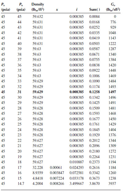
An SRV must be sized to relieve hot water from a water heater at a rate of 20 lbm/s. If the water is at 220°F and 45 psia, what nozzle area in the valve would be required? For the valve, KDL = 0.65 and KDG = 0.98.
Solution:
Assuming the valve discharges into the atmosphere at 14.7 psia, the water (at 220°) will reach its boiling point before leaving the nozzle and will flash in the nozzle. Therefore, we will have a case of all liquid entering the nozzle and a 2-phase liquid/vapor mixture leaving the nozzle. For the solution, we will utilize the HDI method (Equation 11.11), which requires data for the density of the fluid (both water and the water/water vapor mixture) at constant entropy over the range from Po = 45 psia to Pn = 14.7 psia. Such data are available in the steam tables, which can be found in any number of computerized databases. We shall use the NIST Property Database 23, which is easy to use.
The method employs the application of Equation 11.11:
to compute the mass flux, assuming local equilibrium (i.e., a nozzle length over 10 cm long). The procedure is as follows (this is most easily done on a spreadsheet):
1. Use the property database to determine the entropy at the nozzle entrance (Po = 45 psia, To = 220°F, entropy, s = 0.32433 Btu/lbm).
2. Select an appropriate pressure interval (e.g., 1 psia), and use the property database to determine the fluid density (single- or two-phase mixture) at each pressure step, keeping the entropy constant at each step.
3. Decrease Pn in steps and use the database to determine the density at each step.
4. Use the formula from Equation 11.11 to calculate the value of Go at each pressure step, starting with Pn = Po.
5. As Pn is decreased, Go will increase. If the flow is choked, Go will reach a maximum at Pn > Pb = Pc′ and Go = Gc. This is the maximum mass flux that can be obtained, regardless of the downstream exit pressure, Pb. If the exit pressure (Pb) is reached before the maximum in Go is reached, then the flow is not choked and will be sensitive to changes in Pb.
Following this procedure on the spreadsheet, the following results are obtained:
1. A maximum in Go is reached at Pn = 31 psia, where Go = Gc = 1497 lbm/s ft2 (shown in bold in Table 11.1). Because the flow is choked as it leaves the nozzle, the gas/vapor value of KDG = 0.98 should be used to calculate the required nozzle area/diameter:
In practice, the standard nozzle size that is closest to the resulting calculated value, on the high side, is selected (Table E11.2).
Table E11.2
Summary of numerical integration of Equation 11.11
Control valves are used to maintain a desired flow rate, level, temperature or pressure in a process. Control is achieved by automatically adjusting the valve (opened or closed) continuously to achieve a desired flow rate, or other process variable that depends on flow. The valve is controlled by a computer that senses the output signal from a flow meter and adjusts the control valve by pneumatic or electrical signals in response to deviations of the measured flow rate (or other process variable) from a desired set point. A representative flow control system is illustrated in Figure 11.4.
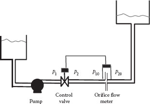
FIGURE 11.4 Schematic of a flow control piping system.
The control valve acts as a variable resistance in the flow line, because closing down on the valve is equivalent to increasing the flow resistance (i.e., the Kf) in the line and vice versa.
The nature of the relationship between the valve stem or plug position (which is the manipulated variable) and the flow rate through the valve, or other process variable, (which is the desired variable) is a nonlinear function of the pressure-flow characteristics of the piping system, the driver (i.e., pump), and the valve trim characteristic, which is determined by the design of the valve plug. This will be illustrated shortly.
There are a large number of types of control valves, and the reader should consult the manufacturers’ literature for details (e.g. Emerson, 2005). A typical globe valve type is illustrated in Figure 11.5.
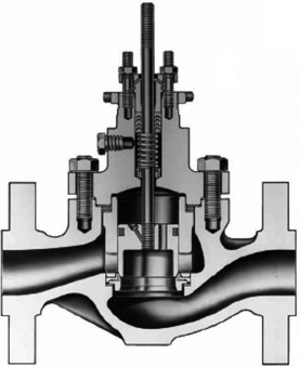
FIGURE 11.5 Valve body with cage-style trim, balanced valve plug. (From Emerson Process Management, Fisher Controls, Control Valve Handbook, 4th edn., Emerson, Process Management, Marshalltown, IA, 2005.)
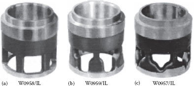
FIGURE 11.6 Characteristic cages for globe-style valve bodies: (a) Quick opening, (b) linear, and (c) equal percentage. (From Emerson Process Management, Fisher Controls, Control Valve Handbook, 4th edn., Emerson, Process Management, Marshalltown, IA, 2005.)
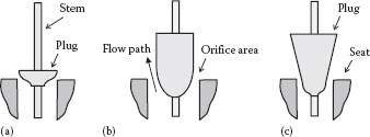
FIGURE 11.7 Valve plug shapes for various trim characteristics: (a) Quick opening, (b) linear, and (c) equal percentage.
For globe valves, different valve plugs (or “cages” that surround the plug) are available for a given valve with a cage-style trim (see Figure 11.6), each providing a different flow response characteristics when the valve setting (i.e., the stem position) is changed. Other valves achieve the desired trim by the shape of the valve plug. A specific valve characteristic must be chosen that, when matched to the response of the pump and the flow system, will give the desired valve stem—system flow response (which is usually desired to be linear). This will be demonstrated later.
Figure 11.6 shows the various “trim cages” that can be inserted in the valve shown in Figure 11.5 to achieve the desired trim. Figure 11.7 shows various valve plug shapes that result in different trim characteristics. Figure 11.8 illustrates the flow versus valve stem travel characteristic for various typical valve trim functions (Emerson, 2005). The quick opening characteristic provides the maximum change in flow rate at low opening or stem travel with a fairly linear characteristic. As the valve approaches the wide-open position, the change in flow with stem travel approaches zero. This is best suited for on-off control but is also appropriate for some applications where a linear response is desired.
The linear flow characteristic has a constant “valve gain,” that is, the incremental change in flow rate with the percentage change in the valve plug position is the same at all flow rates. This is the most commonly desired characteristic.
The equal percentage trim provides the same percentage change in flow for equal increments of the valve plug position. With this characteristic, the change in flow is always proportional to the value of the flow rate just before the change is made. This characteristic is used in pressure control applications and where a small pressure drop across the valve is required relative to that in the rest of the system.
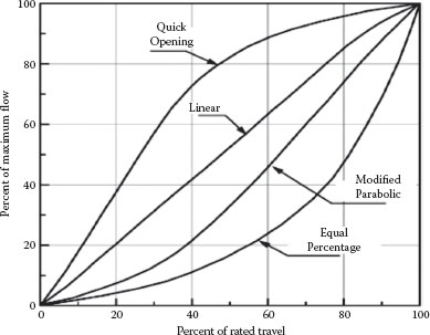
FIGURE 11.8 Various valve trim characteristics.
The modified parabolic characteristic is intermediate to the linear and equal percentage characteristics and can be substituted for equal percentage valve plugs in many applications, with some loss in performance.
Some general guidelines for the application of the proper valve characteristics are shown in Table 11.1. These are rules of thumb, and the proper valve response can be determined only by a complete analysis of the system in which the valve is to be used (see also Baumann (1991) for simplified guidelines). We will illustrate later how the valve trim characteristic interacts with the pump and system characteristics to affect the flow rate in the system and how to use this information to select the most appropriate valve trim.
B. OVERVIEW OF CONTROL VALVE SIZING
The basic principle that governs the flow through a control valve is the same as that through an orifice, that is, the engineering Bernoulli equation as applied to an orifice. However, there are several important characteristics of control valves that are fundamentally different from an orifice that must be accounted for, namely:
• There is no one specific flow area in a control valve that can serve as a reference area, such as that in an orifice or relief valve. Consequently, the “flow area” and the coefficient of discharge are combined into one parameter, which is not dimensionless.
• The reference pressure drop through the valve is the total net pressure drop, instead of the pressure drop to the vena contracta as in the orifice. This total net pressure drop (P1 − P2) is also referred to as the “service pressure drop.” This requires that the pressure recovery in the valve outlet body be accounted for, as it is the pressure drop to the vena contracta that determines the flow rate, and not the service pressure drop.
• For compressible flow, the choke pressure has a unique definition, which is not necessarily the same as the actual choke pressure.
• The definition of the expansion coefficient (Y) is a variation of that used for the orifice.
TABLE 11.1
Guidelines for Control Valve Applications
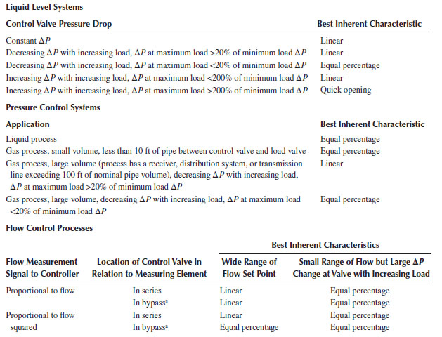
Source: Emerson Process Management, Fisher Controls, Control Valve Handbook, 4th edn., Emerson, Process Management, Marshalltown, IA, 2005.
a When control valve closes, flow rate increases in the measuring element.
The general approach to sizing a control valve is to consider it as an orifice and then apply various “correction factors” to account for the deviation of the valve flow from flow through an actual orifice. This involves lumping parameters for the valve that are not uniquely defined and applying empirical correction factors to account for them. Clearly, from inspection of Figure 11.5, these correction factors must be very important because of the significant deviation of the valve geometry from that of the orifice.
Just as for the relief valve, the starting point for all geometries, incompressible, compressible, and two-phase flows, is the general steady-state Bernoulli equation (Equation 11.2) for the mass flux through the valve:
(11.2) |
This can be rearranged to solve for the mass flow rate, with inclusion of the “discharge coefficient” (Cd) to account for deviations from ideal orifice flow:
(11.16) |
Here, β = do/D, where do is the orifice diameter and D is the pipe diameter. For the valve, do, and hence Ao, is not uniquely defined so that the discharge coefficient and the beta geometrical term are combined into a single “flow coefficient,” Kd or Co:
(11.17) |
The “effective area” in Equation 11.16 is AoKd =F(Cv/38) where Cv is the valve coefficient and F = FL for liquid flow and F = FG for gas flow. F is a dimensionless correction factor that is applied to account for the pressure recovery from the vena contracta (Pvc) to P2 (hence to the service pressure drop (P1 − P2), as discussed below).
Notation: Because of the variety of notation used by different references, there is no single universal standard. The two most definitive references for control valve sizing and selection are those of Emerson (2005) and ISA (2012) as well as IEC (2011). Because of its longer standing in the field and common usage in earlier publications, the Emerson notation is still frequently used. However, the IEC/ISA notation is gradually becoming the accepted standard. The most common terms and their definitions are given in the section “Notation” at the end of this chapter.
Because of the complex combinations of units, as well as the different systems of units employed, most of the equations require various combinations of conversion factors to give the desired units. To facilitate the conversion of units, many of the equations from IEC/ISA and Emerson (2005) include an “equation constant,” N, which incorporates the various conversion factors needed in that equation for the desired net units. This applies to “American (English) engineering” units, as well as metric units. A listing of these equation constants is given in Table 11.2. This table is not exhaustive, as there are other combinations of units that may be encountered, such as those in Equation 11.16.
For incompressible fluids, Equation 11.16 can be written as
(11.18) |
TABLE 11.2
Equation Constantsa
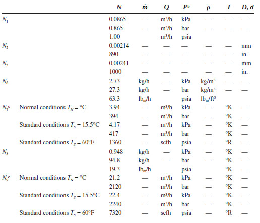
Source: Emerson Process Management, Fisher Controls, Control Valve Handbook, 4th edn., Emerson, Process Management, Marshalltown, IA, 2005.
a Many of the equations used in the sizing procedures contain a numerical constant, N, along with a numerical subscript. These numerical constants provide a means for using different units in the equations. Values of the numerical and the appropriate units are given in this table. For example, if the flow rate is given in the U.S. gpm and the pressure in psia, N1 has a value of 1.00. If the flow rate is m3/hr and the pressure is in kPa, the N constant is 0.0865.
b All pressures are absolute.
c The base pressure is 101.3 kPa or 1.013 bar or 14.7 psia.
where Cv is a combination of the coefficients and parameters in Equation 11.16 and is called the valve sizing coefficient. This is explained in the following section. The term AoKd is assumed to be an “effective flow area” for the valve, which when compared with the equivalent IEC/ISA expression, shows that AoKd = FLCv / 38. There are a variety of correction factors or coefficients that are applied to the flow equation for incompressible fluids to account for deviation from the ideal orifice model, and these are shown in Table 11.2 and described in the following.
1. The Valve Sizing Coefficient
The coefficient Cv in Equation 11.18 is the valve sizing coefficient and accounts for deviations from ideal incompressible orifice flow in the valve. Note that Cv is not dimensionless, as it incorporates all of the numerical coefficients in Equation 11.16, including the effective flow area AoKd, which is an unknown geometrical parameter for the valve. This coefficient is also identified by other symbols in various references (e.g., C, Kv, Av, etc.). It is determined empirically by the manufacturer, and representative values are given in the manufacturers’ handbook (e.g., Emerson, 2005) or the ISA Handbook (1971), as shown in Table 11.3. If Equation 11.18 is written for the volumetric flow rate (Q) instead of the mass flow rate, it can be expressed as
(11.19) |
where
SGL is the specific gravity of the flowing fluid relative to a standard (i.e., water at 60°F = 62.3 lbm/ft3)
hv is the “head loss” across the valve, in ft (of fluid)
The value of the reference fluid density is included in the definition of Cv.
The units normally used in the United States are the typical “American (English) Engineering” units, as follows:
ṁ is the mass flow rate (liquid or gas) (lbm/h).
Q is the volumetric flow rate (gpm for liquids or scfh for gas or steam).
TABLE 11.3
Example Flow Coefficient Values for a Control Valve with Various Trim Characteristics
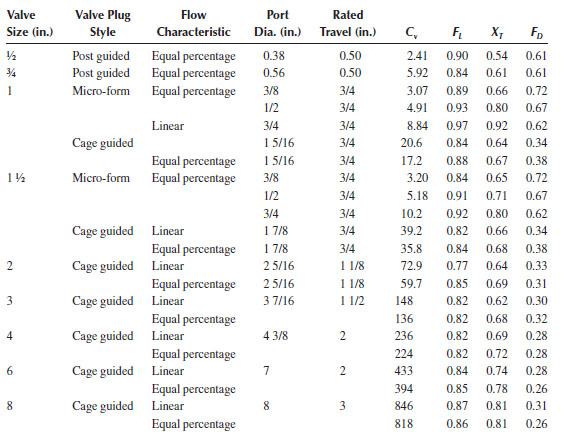
Source: ISA, (2012).
SGL, SGG is the specific gravity [relative to water for liquids (62.3 lbm/ft3) or air at 60° and 1 atm for gases (0.0764 lbm/ft3)].
ρ1 is the density at upstream conditions (lbm/ft3).
P1 is the upstream pressure (psia).
ΔP is the total (net recovered “service”) pressure drop across valve (psi).
There are a number of combinations of other “engineering” or “metric” units that are also used with these equations (e.g., gpm, psi, scfh, lbm/h, lbm/ft3, m3/h, kPa, bar, etc.), and for each combination of units there is a specific value of the combined conversion factors that satisfy the equations. For example, the most common units associated with Cv in “American (English) engineering units” are gpm/(psi)1/2. If the fluid density were to be included in Equation 11.19 instead of the specific gravity (SGL), the dimensions of Cv would be [L2], reflecting the inclusion of the unknown factor Ao in Cv (i.e., Cv = 38AoKd/FL). The “usual American engineering units” will be indicated in most of the working equations, along with the net numerical values of the conversion factors required to satisfy the equation.
2. FP: The Piping Geometry Factor
It often occurs that the nominal size of the control valve that is best for a given application is smaller than the pipe in which it is installed (i.e., there is a pipe reducer upstream of the valve and a pipe expander downstream), and/or there may be other fittings such as elbows, tees, etc., attached to the valve. In this case, the piping geometry factor, FP, must be applied. It is a dimensionless factor and is often determined empirically by the manufacturer and reported in the tables such as Table 11.3. Otherwise, it is determined from the following equation (Emerson, 2005):
(11.20) |
where
d is the nominal valve size
Cv is the valve sizing coefficient at 100% stem travel
The term ΣKf is the sum of all friction loss factors for any upstream and downstream fittings and also includes the upstream and downstream kinetic energy loss factors:
(11.21) |
where D is the pipe ID. Obviously, if the upstream and downstream piping are the same size, these terms cancel. For other combinations of fittings, see Emerson (2005) or Chapter 7 in this book.
3. : The Liquid Pressure Recovery Factor
The total (measured) pressure drop across the valve, or service pressure drop (P1 − P2) in Equation 11.19 and Figure 11.9 omit) is the overall (recovered) pressure drop. This is not the maximum pressure drop across the valve (or orifice), however, which is (P1 − Pvc) where Pvc is the pressure at the vena contracta.
In order to account for the difference between the (measured) pressure downstream of the valve (P2) and the lower pressure just downstream at the vena contracta, (Pvc), as well as the pressure recovery downstream, a dimensionless correction factor FL called the liquid recovery factor is defined as
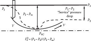
FIGURE 11.9 Vena contracta correction factor.
TABLE 11.4
Representative Full-Open Values for Various Valves
Body Type |
|
Globe: single port, flow opens |
0.70–0.80 |
Globe: double port |
0.70–0.80 |
Angle: flow closes |
|
Venturi outlet liner |
0.20–0.25 |
Standard seat ring |
0.50–0.60 |
Angle: flow opens |
|
Maximum orifice |
0.70 |
Minimum orifice |
0.90 |
Ball valve |
|
v-notch |
0.40 |
Butterfly valve |
|
60° open |
0.55 |
90° open |
0.30 |
(11.22) |
Values of the liquid recovery factor are determined by the valve manufacturer, as shown in Table 11.3, and are assumed to be constant regardless of the pressure drop. Note that different symbols are used in various references for the same correction factor (e.g., ). The notation FL is from the ANSI/ISA 75.01.01/IEC-60534-2-1 (2012) standard and Km is that of Emerson/Fisher Controls (1990). This dimensionless factor is determined by the manufacturer for each control valve, and is assumed to be constant regardless of the pressure drop. Typical values of FL are shown in Tables 11.3 and 11.4.
4. Fd: The Valve Style Modifier
Fd is the dimensionless ratio of the hydraulic diameter of a single flow passage to the diameter of a circular orifice, the area of which is equivalent to the sum of areas of all identical flow passages at a given travel. It is normally given by the manufacturer as a function of stem travel.
Example 11.3 Liquid Valve Sizing Example (Emerson, 2005)
Consider an installation that, upon start-up, will not be operating at full capacity. The lines are sized for the ultimate system capacity, but it is desired to install a control valve sized for currently anticipated requirements. The line size is 8 in., and a Class 300 globe valve with an equal percentage cage has been specified. Standard concentric reducers will be used to install the valve in the line. Determine the appropriate valve size.
Solution:
The following operating conditions are specified:
• Valve design: Class 300 globe valve with equal percentage cage and an assumed size of 3 in.
• Fluid: Liquid propane
• Service conditions:
• Q = 800 gpm
• P1 = 300 psig = 314.7 psia
• P2 = 275 psig = 289.7 psia
• ΔP = 25 psi
• T1 = 70°F
• SGf = 0.5
• Pv = 124.3 psia
• Pc = 616.3 psia
From Table 11.2, N1 = 1.
Determine the piping geometry factor, FP. This accounts for the fitting losses for the 3 in. valve installed in an 8 in. line:
where N2 = 890 from Table 11.2, and d = 3 in.
From the flow coefficient table for a Class 300 3 in. globe valve with equal percentage cage, Cv = 121. For a valve installed between two identical reducers:
Therefore,
Determine ΔPmax (the allowable sizing pressure drop). Based on the small required pressure drop, the flow will not be choked (ΔPmax > ΔP).
Solve the liquid flow equation for Cv:
The valve size based on this value of Cv and the tables for the flow coefficient show that it is larger than the assumed value of Cv = 121. Thus, the calculation is repeated assuming the next larger valve size of 4 in., having a Cv of 203. This yields the following results: ΣK = 0.84, FP = 0.93, and Cv = 116.2. Thus, the proper valve size would be between 3 and 4 in., so the 4 in. valve opened to about 75% of total travel should be adequate.
E. CAVITATING AND FLASHING LIQUIDS
The minimum pressure in the valve (Pvc) generally occurs at the vena contracta, just downstream of the flow orifice. The pressure then rises downstream to P2 (as shown in Figure 11.9), with the amount of pressure recovery depending upon the valve design. If the downstream choke pressure (Pc) is less than the fluid vapor pressure (Pv), the liquid will partially vaporize forming bubbles. This is sometimes described as “liquid choking,” although liquids do not “choke” as such. Anytime the local pressure falls below the vapor pressure of the liquid it will “flash” or vaporize, resulting in vapor or two-phase flow, which may choke. At the “choke point,” a further drop in the downstream pressure will not increase the flow rate any further. An increased pressure drop (P1 − Pc) may be due to an increase in temperature or velocity (i.e., cavitation).
If the pressure recovers to a value greater than Pv, these bubbles may collapse suddenly, setting up local shock waves, which can result in considerable damage to the valve. This condition is referred to as cavitation (similar to that seen in centrifugal pumps), as opposed to flashing that occurs if the recovered pressure (P2 = Pc) remains below Pv so that the vapor does not condense. After the first vapor cavities form, the flow rate will no longer be proportional to the square root of the pressure difference across the valve because of the decreasing density of the mixture. If sufficient vapor forms, the flow can become choked, at which point the flow rate will be independent of the downstream pressure as long as P1 remains constant.
2. FF = rc: The Liquid Critical Pressure Ratio
The critical pressure ratio P2/Pv = Pc/Pv = rc is that at which the liquid will vaporize resulting in possibly damaging cavitation or flashing, resulting in choked flow. The corresponding maximum flow rate through the valve at that point is
(11.23) |
where
Pv is the vapor pressure of the fluid
rc represents the choke pressure
SGL is its specific gravity (relative to water)
Note that the reference density of water must then be included in the “conversion factors” required for the units used in Equation 11.23.
For pure components, the choke pressure may be estimated as rcPv and values for FF = rc can be determined from the following correlation:
(11.24) |
where Ptc is the thermodynamic (absolute) critical pressure for the fluid. Figure 11.10 shows the correlation of rc for water, and Figure 11.11 shows the correlation for other fluids. Table 11.5 gives the thermodynamic critical temperature for various fluids. However, the correlation in Equation 11.24 was derived for pure components and it may overstate the choke pressure for multicompound fluids, thus resulting in an undersized control valve. The determination of the choke pressure for multicomponent systems (or any system) may be determined more easily using the HDI method (see Section 4).
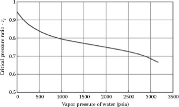
FIGURE 11.10 Critical pressure ratio for water. The abscissa is the water vapor pressure at the valve inlet. The ordinate is the corresponding critical pressure ratio, rc = FF. (From Emerson Process Management, Fisher Controls, Control Valve Handbook, 4th edn., Emerson, Process Management, Marshalltown, IA, 2005.)
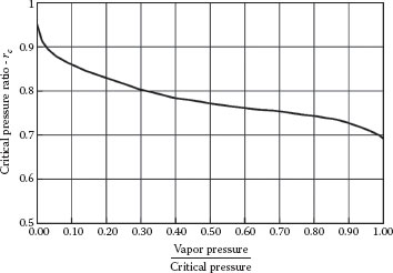
FIGURE 11.11 Critical pressure for cavitating and flashing liquids other than water. The abscissa is the ratio of the liquid vapor pressure at the valve inlet divided by the thermodynamic critical pressure of the liquid. The ordinate is the corresponding critical pressure ratio, rc = FF (From Emerson Process Management, Fisher Controls, Control Valve Handbook, 4th edn., Emerson, Process Management, Marshalltown, IA, 2005.)
To determine if cavitation will occur, the cavitation pressure is determined from the choke pressure (Pc):
(11.25) |
Thermodynamic Critical Pressure of Various Fluids (psia)
Ammonia |
1636 |
Argon |
705.6 |
Butane |
550.4 |
Carbon dioxide |
1071.6 |
Carbon monoxide |
507.5 |
Chlorine |
1118.7 |
Dowtherm A |
465 |
Ethane |
708 |
Ethylene |
735 |
Fluorine |
808.5 |
Helium |
33.2 |
Hydrogen |
188.2 |
Hydrogen chloride |
1198 |
Isobutane |
529.2 |
Isobutylene |
580 |
Methane |
673.3 |
Nitrogen |
492.2 |
Nitrous oxide |
1047.6 |
Oxygen |
736.5 |
Phosgene |
823.2 |
Propane |
617.4 |
Propylene |
670.3 |
Refrigerant 11 |
635 |
Refrigerant 12 |
596.9 |
Refrigerant 22 |
716 |
Water |
3206.2 |
The proper pressure drop to use in the liquid sizing equation depends on cavitation, as follows:
• If the overall “service” pressure drop (P1 − P2) is less than ΔPcav, or if the pressure at the vena contracta (Pvc) is greater than the choke pressure (Pc), then the fluid will not cavitate or choke
• If the overall service pressure drop (P1 − P2) is greater than ΔPcav, or if the pressure at the vena contracta (Pvc) is less than the choke pressure (Pc), then the fluid will choke and the cavitation pressure drop is to be used in the valve equation to determine Q:
(11.26) |
• Otherwise, the total pressure drop (P1 − P2) is used.
The notation used here is that of the Emerson/Fisher literature (e.g., Emerson, 2005). The ANSI/ISAS75.01 standard for control valves uses the same equations, except that it uses the notation and FF = rc in place of the factors Km and rc, respectively.
This parameter provides the same information as FF = rc. Specifically, xT is the dimensionless pressure drop ratio [xT = (P1 − Pc)/P1] required to produce critical or maximum (flashing) flow through the valve when Fk = 1 (where Fk = k/1.4 is the specific heat ratio factor). Values of xT are provided by the manufacturer, as shown in Table 11.4.
1. Fv: The Viscosity Correction Factor
A correction for fluid viscosity must be applied to the flow coefficient (Cv) for liquids other than water. This viscosity correction factor (Fv) is obtained from Figure 11.12 by the following procedure, depending upon whether the objective is to find the valve size for a given Q and ΔP, to find Q for a given valve and ΔP, or to find ΔP for a given valve and Q.
1. To find valve size
For the given Q and ΔP, calculate the required Cv as follows:
(11.27) |
Then determine the Reynolds number from the equation:
(11.28) |
where
Q is in gpm
ΔP is in psi
vcs is the fluid kinematic viscosity (νcs = μ/ρ, in centistokes)
The viscosity correction factor, Fv, is then read from the middle line on Figure 11.12 and used to correct the value of Cv as follows:
(11.29) |
2. To predict flow rate
For a given valve (i.e., a given Cv) and given ΔP, the maximum flow rate (Qmax) is determined from
(11.30) |
The Reynolds number is then calculated from Equation 11.28, and the viscosity correction factor, Fv, is read from the bottom curve in Figure 11.12. The corrected flow rate is then
(11.31) |
3. To predict pressure drop
For a given valve (Cv) and given flow rate (Q), calculate the Reynolds number from Equation 11.28 and read the viscosity correction factor, Fv, from the top line of Figure 11.12. The predicted pressure drop across the valve is then
(11.32) |
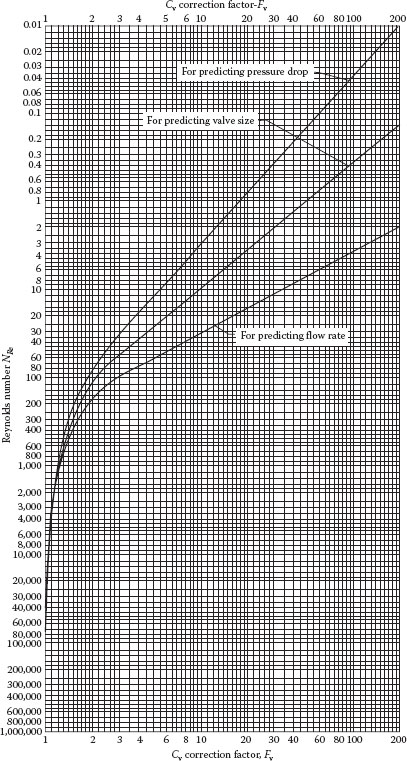
FIGURE 11.12 Viscosity correction factor for Cv. (From Emerson Process Management, Fisher Controls, Control Valve Handbook, 4th edn., Emerson, Process Management, Marshalltown, IA, 2005.)
Just as for incompressible flows, the overall pressure drop (ΔP = P1 − P2) is used in the sizing equation, with a correction factor to account for the effect of the vena contracta (Pvc), defined as
(11.33) |
• For high-recovery control valves (low Cv and XT), the value of FG is less than one and the choking pressure drop at the vena contracta (P1 − Pvc) is greater than the overall pressure drop (P1 − P2).
• For large-pressure drop control valves with minimum recovery (large Cv and XT), the value of FG is greater than one and the choking pressure drop at the vena contracta (P1 − Pvc) is less than the overall pressure drop (P1 − P2). An example is the doubleported globe valve.
The general formula for gas flow valve sizing is thus
(11.34) |
where the range of integration is from the valve inlet pressure, P1, to the vena contracta pressure at the valve exit, Pvc, which is related to P2 by Equation (11.33). This is less than the downstream pressure, P2, because of the pressure recovery downstream of Pvc. The term A0Kd represents the “effective flow area,” and is found by comparing the integrated Bernoulli equation with the corresponding IEC/ISA expression, yielding AoKd = FGCv/38.
To determine the value of the gas pressure-adjustment coefficient FG, the parameter (AoKd) is assumed constant. This is a good assumption if the Reynolds number based on the upstream flow area is greater than 100,000. The value of FG is related to other valve correction factors by
(11.35) |
since
where γ = Cp/Cv = k, and
(11.36) |
FG is not strongly dependent upon the value of γ, as a variation in γ of 50% results in a variation in FG of approximately 4%. Here, Cγ and Fγ are a consolidation of terms that are functions only of γ:
(11.37) |
and
(11.38) |
The factor XT is based on air near atmospheric pressure as the flowing fluid with a specific heat ratio of 1.40. If the specific heat ratio for the flowing fluid is not 1.40, the factor Fγ = γ/1.4 is used to adjust XT, as in Equation 11.35.
Equation 11.34 evolved from the assumption of perfect gas behavior and extension of the orifice plate model, based on air and steam testing on control valves. Analysis of that model over a range of 1.08 < γ < 1.65 has led to the adoption of the current linear model embodied in Equation 11.34. The difference between the original orifice model, other theoretical models, and Equation 11.34 is small within this range. However, the differences become significant outside of the indicated range. For maximum accuracy, the flow calculations based on this model should be restricted to a specific heat ratio within this range and to ideal gas behavior.
For relatively low pressure drops (i.e., less than about 30%), the effect of compressibility is negligible and the general incompressible flow equation (Equation 11.18) may be applied. Introducing the conversion factors to give the flow rate in standard cubic feet per hour (scfh) and the density of air at standard conditions (1 atm, 520°R), Equation 11.18 becomes
(11.39) |
The effect of variable density can be accounted for by an expansion factor Y (Hutchinson, 1971), as has been done for flow in pipes and orifice meters (see Chapter 10), in which case Equation 11.39 can be written as
(11.40) |
where
(11.41) |
Here, SG is defined as MW/28.9655, and Qscfh = W(lbm/h) [379.49 scf/lbmol]/M(lbm/lbmol) at 14.696 psia and 60°F.
The expansion factor Y depends on the pressure drop X, the dimensions (clearance) in the valve, the gas specific heat ratio k = γ, and the Reynolds number (the effect of which is often negligible). It has been found from measurements (Hutchison, 1971) that the expansion factor for a given valve can be represented, to within about ±2%, by the expression
(11.42) |
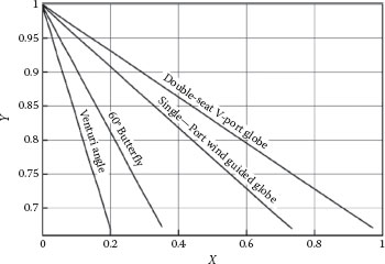
FIGURE 11.13 Expansion factor (Y)—as a function of pressure drop ratio (X) for four different types of control valves. (From Hutchinson, J.W., ISA Handbook of Control Valves,1st edn., Instrument Society of America, Durham, NC, 1971.)
where XT is specific to the valve at the choke point, as illustrated in Figure 11.13. Deviations from the ideal gas law can be incorporated by multiplying T1 in Equation 11.39 or 11.40 by the compressibility factor, Z, for the gas.
When the gas velocity reaches the speed of sound, choked flow occurs and the mass flow rate reaches a maximum. It can be shown from Equation 11.42 that this is equivalent to a maximum in YX1/2, which occurs at Y = 0.667 and corresponds to the terminus of the lines in Figure 11.13. That is, XT is the pressure ratio across the valve at which choking occurs, which is determined empirically. At the choke point, any further increase in X (e.g., ΔP) due to lowering P2 can have no effect on the flow rate.
The flow coefficient Cv is determined by calibration with water, and it is not entirely satisfactory for predicting the flow rate of compressible fluids under choked flow conditions. This has to do with the fact that different valves exhibit different pressure recovery characteristics with gases and hence will choke at different pressure ratios, which does not apply to liquids. For this reason, another flow coefficient, Cg, is often used for gases and is determined by calibration with air under critical flow conditions (Emerson, 2005). The corresponding flow equation for gas flow is
(11.43) |
H. GENERAL (HDI) METHOD FOR ALL FLUIDS AND ALL CONDITIONS
There are many other factors or coefficients that may be applied to the basic equation to account for gas flow, cavitation, flashing, etc. However, regardless of whether the fluid is a liquid, gas or vapor, or single- or two-phase flashing flow, the flow rate can be calculated directly by a simple numerical integration (HDI) of the basic integral form of the Bernoulli equation, provided a thermodynamic fluid property database is available for the fluid properties. All that is needed is the density of the fluid or the mixture as a function of pressure over the pressure range of interest. As mentioned for safety valves, there are many such databases available. A handy and easy-to-use inexpensive database containing hundreds of fluids (and some two-phase systems) is the NIST REFPROP, (2015) database.
The method is based on the integration of the differential form of the Bernoulli equation. For liquids, the equation is
(11.44) |
where Ao(in.2)Kd = (FLCv/38) (in.2). The equivalent ISA and Fisher notation for the gas flow coefficients is shown in Table 11.6.
Note that the range of integration is from P1 to Pvc, the pressure at the vena contracta, which is assumed to exist at the valve exit. This is lower than the pressure P2, which is the “recovered” pressure downstream of the valve. The value of the vena contracta pressure for liquids can be determined from the parameter as defined by Equation 11.22:
(11.22) |
which can be used to convert (P1 − Pvc) to the service pressure drop, (P1 − P2).
Equation 11.44 can be written in numerical form to apply from the upstream pressure (P1) to the minimum exit pressure at the vena contracta:
(11.45) |
(11.46) |
where the summation is along an isentropic path from P1 to Pvc. In practice, the summation starts with a vena contracta pressure just below P1 and proceeds until the value of Pvc is reached. If the flow is choked, the mass flow rate will reach a maximum before the pressure reaches Pvc, in which case no further reduction of Pvc will result in an increase in flow rate.
Equivalent Parameters for AoKd for Gases
ISA parameters |
{A0Kd} = 12.873 [Cv/Cγ] [XT Fγ)½] |
{A0Kd} = [(Cv/38)] [489.174 (XT Fγ)½/Cγ] |
Fisher parameters |
{A0Kd} = [Cg/1100] |
{A0Kd} = [Cv * C1/1100] |
{A0Kd} = [Cv/38] [C1/28.9] |
For compressible fluids, an analogous form of Equation 11.44 is
where the vena contracta pressure can be determined by using the parameter FG2, given by Equation 11.33:
(11.33) |
which is analogous to Equation 11.22 for liquids. The effective flow area is:
(11.47) |
The pressure drop (P1 − Pvc) can be converted to the service pressure drop (P1 − P2) by Equation 11.33. This method can be applied directly to all cases, including incompressible, compressible, single- and two-phase flows, flashing and cavitating flows, etc., as long as the requisite fluid properties (i.e., ρ(P)) are available. For two-phase flow, if the flow is choked the value of A0Kd for gas flow should be used, but if the flow is not choked the liquid value should be used.
It should be noted that the vena contracta for gases is significantly different than for liquids, due to the rapid expansion of the gas as it leaves the valve. Also, if the flow is choked as it leaves the valve (as is the usual case), no further pressure drop or any change in conditions downstream of that point will affect the flow rate, so it is important to initially determine if the flow is choked. Although the methods outlined previously are recommended in the literature, it is generally easier and more accurate to use the HDI method for these more complex situations when possible.
In the case of two-phase flow, the question arises as to whether to use FL or FG to relate Pvc to P2. For many valves, there is little difference between these two, but where there is, logic would indicate a preference for using FG.
Example 11.4 Valve Sizing for Compressible Fluids Using the Fisher/Emerson Method (Emerson 2005)
Steam is to be supplied to a process that is to operate at 250 psig. The steam is supplied from a header at 500 psig and 500°F. A 6 in. line from the header to the process is planned. If the required control valve calculated is less than 6 in., it will be installed using concentric reducers. Determine the appropriate Design ED valve with a linear cage.
Specify the Necessary Design Variables
(a) Desired valve: Class 300 Design ED valve with a linear cage. Assume a 4 in. valve.
(b) Process fluid: Superheated steam.
(c) Conditions: ṁ = 125,000 lbm/h, P1 = 500 psig = 514.7 psia, P2 = 250 psig = 264.7 psia, ΔP = 250 psi, x = ΔP/P1 = 250/514.7 = 0.49, T1 = 500°F, γ1(ρ1) = 1.0434 lbm/ft3 (from steam tables), k = 1.28 (from steam tables).
(d) Determine equation constants from equation constants (N) table—because the flow rate and density are in mass units (lbm/h and lbm/ft3), and the pressure is in psi, the appropriate equation constant is N6 = 63.3.
(e) Determine the piping geometry factor
where
N2 = 890 (from equation constants table)
d = 4 in.
Cv = 236 (from the manufacturer’s flow coefficient table for a 4 in. Design ED valve at 100% travel).
and
Also
(f) Determine the expansion factor, Y:
where Fk = k/1.40 = 1.28/1.40 = 0.91, x = 0.49 (from given pressures).
Because the 4 in. valve is to be installed in a 6 in. line, the xTP is given by
where
N5 =1000, from equation constants table
d = 4 in., Fp = 0.95 (step e.)
xT = 0.688 (from the manufacturer's flow coefficient table)
Cv = 236 (from step e.) and
where D = 6 in.
So
(g) Calculate Cv:
(h) Select the valve size from the manufacturer’s flow coefficient table for Design ED valves with a linear cage and the calculated value of Cv. The assumed 4 in. valve has a Cv of 236 at 100% travel and the next smaller size (3 in.) has a Cv of 148, so the assumed size is correct. If the calculated value of Cv had been small enough to be handled by the 3 in. valve, or larger than the rated Cv for the assumed size, it would be necessary to rework the problem with a new assumed size.
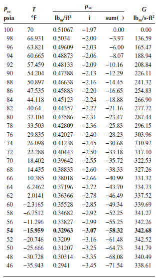
Example 11.5 Valve Sizing for Compressible Fluids using the HDI Method
A control valve is to be sized to control the flow rate of air through a pipeline. The pressure upstream of the valve is 100 psia at a temperature of 70°F, and the discharge pressure is 14.7 psia. The valve to be used is a 3 in. high recovery Venturi ball valve, with the following parameters:
Determine the maximum flow rate of air that this valve can handle, in lbm/h, using the HDI method.
Solution: The basic equation that governs this system is Equation 11.46:
where the “hypothetical” mass flux (G) through the valve is given by G = ṁ/AoKd.
The first step is to determine the density of air at 70°F and 100 psia, and over the pressure range of interest at constant entropy, using a fluid property database such as NIST REFPROP, (2015 or later). A suitable pressure interval (e.g. 2 psi) is used, starting at P1 = 100 psi. This will give the density of air from P1 = 100 psia to 14.7 psia in increments of 2 psi. These data can now be used to calculate the summation term in the above equation, for each pressure increment from Pt to (Pvc),i. Thus the mass flux and the flow rate can be calculated from the above equation for each value of (Pvc)i. These values are shown in bold face in Table E11.5.
It is seen that the flow is choked at about Pvc = 54 psia, with a mass flux of 343 lbm/s ft.2, or a total mass flow rate of:
The pressure at the vena contracta can be converted to the equivalent discharge “service” pressure using the factor FG from Equation 11.33:
Given that P1 = 100 psia, a discharge vena contracta pressure of Pvc = 14.7 psia corresponds to a discharge service pressure of P2 = 79.8 psia, and a choke pressure of Pvcchoke = 54 psia corresponds to P2c = 89.1 psia.
Spreadsheet Output for Example 11.5
In normal operation, a linear relation between the manipulated variable (valve stem position) and the desired variable (flow rate) is desired. However, the valve is normally a component of a flow system that includes a pump or other driver, pipe, and fittings characterized by loss coefficients, as illustrated in Figure 11.4. In such a system, the flow rate is a nonlinear function of the component loss coefficients. Thus, the control valve must have a nonlinear response (i.e., trim) to compensate for the nonlinear system characteristics if a linear response is to be achieved. Selection of the proper size and trim of the valve to be used for a given application requires matching the valve, piping system, and pump characteristics, all of which interact (Darby, 1997). The operating point for a piping system depends upon the pressure-flow behavior of both the system and the pump, as described in Chapter 8 and illustrated in Figure 8.2 (see also Example 8.1). The control valve acts like a variable resistance in the piping system. That is, as the valve is closed, the valve loss coefficient Kf increases and the valve sizing coefficient Cv decreases. The operating point for the system is where the pump head (Hp) characteristic intersects the system head requirement (Hs):
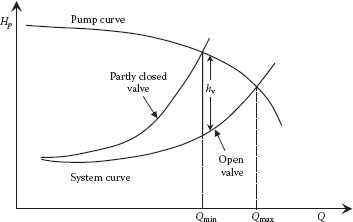
FIGURE 11.14 Effect of control valve on system operating point.
(11.48) |
where the last term in the brackets is the head loss through the control valve, hv, from Equation 11.19, and Cv depends upon the valve stem travel, X (e.g., Figure 11.8):
(11.49) |
A typical situation is illustrated in Figure 11.14, which shows the pump curve and a system curve with no control valve, and the same system curve with a valve that is partially closed. Closing down on the valve (i.e., reducing X) decreases the valve Cv and increases the head loss (hv) through the valve. The result is to shift the system curve upward by an amount hv at a given flow rate (note that hv also depends on the flow rate). The range of possible flow rates for a given valve (also known as the “turndown” ratio) lies between the intersection on the pump curve of the system curve with a “fully open” valve (Qmax, corresponding to Cv,max) and the intersection of the system curve with the (partly) closed valve. Of course, the minimum flow rate is zero when the valve is fully closed. The desired operating point should be as close as possible to Qmax, because this corresponds to an open valve with minimum flow resistance. The flow is then controlled by closing down on the valve (i.e., reducing X and Cv and thus raising hv). The minimum operating flow rate (Qmin) is established by the turndown ratio (i.e., the operating range) required for proper control. These limits set the size of the valve (e.g., the required Cv,max), and the head flow rate characteristic of the system (including pump and valve) over the desired flow range. This determines the proper trim for the valve, as follows. As the valve is closed (i.e., reducing X), the system curve is shifted up by an amount hv:
(11.50) |
where f(X) represents the valve trim characteristic function. Equation 11.50 follows directly from Equations 11.19 and 11.49. Thus, as X (the relative valve stem travel) is reduced, f(X) and Cv are also reduced. This increases hv, with the result that the system curve now intersects the pump curve further to the left, at a lower value of Q. Substituting Equation 11.50 into Equation 11.48 gives
(11.51) |
which relates the system required head (Hs) to the valve stem position (X).
J. MATCHING VALVE TRIM TO THE SYSTEM
The valve trim function is chosen to provide the desired relationship between the valve stem travel (X) and flow rate (Q). This is usually a linear relation and/or a desired sensitivity of the flow rate to a change in valve stem position. For example, if the operating point were far to the left on the diagram where the pump curve is fairly flat, then hv would be nearly independent of flow rate. In this case, Q would be proportional to Cv = Cv,max f(X), and a linear valve characteristic [f(X) vs. X] would be desired. However, the operating point usually occurs where both curves are nonlinear, so that hv depends strongly on Q, which in turn is a nonlinear function of the valve stem position, X. In this case, the most appropriate valve trim can be determined by evaluating Q as a function of X for various trim characteristics (e.g., Figure 11.8) and choosing the trim that provides the most linear response over the desired operating range. For a given valve (e.g., Cv,max), and a given trim response (e.g., f(X)), this can be done by calculating the system curve (e.g., Equation 11.51) for various valve settings (X) and determining the corresponding values of Q from the intersection of these curves with the pump curve (e.g., the operating point). The trim that gives the most linear (or most sensitive) relation between X and Q is then chosen. This process can be aided by fitting the trim function (e.g., Figure 11.8) by an empirical equation such as the following (Darby, 1997):
(11.52) |
(11.53) |
(11.54) |
(11.55) |
where a and n are parameters that can be adjusted to give the best fit to the trim curves.
Likewise, the pump characteristic can usually be described by a quadratic equation of the form
(11.56) |
The operating point is where the pump head (Equation 11.56) intersects the system head requirement (Equation 11.51). Thus, if Equation 11.51 for the system head is set equal to Equation 11.56 for the pump head, the result can be solved for 1/f(X)2 to give
(11.57) |
where conversion factors have been included for units of Q in gpm, Ho, Δz and ΔP/ρg in ft, Din in in.; and Cv,max in (gpm/psi1/2). The valve position X corresponding to a given flow rate Q is determined by equating the value of f(X) obtained from Equation 11.57 to that corresponding to a specific valve trim, for example, Equations 11.52 through 11.55. This procedure is illustrated by the following example.
Example 11.6 Control Valve Trim Selection
It is desired to find the trim for a control valve that gives the most linear relation between the stem position (X) and flow rate (Q) when used to control the flow rate in the fluid transfer system shown in Figure 11.14. The fluid is water at 60°F, through 100 ft of 3 in. sch 40 pipe containing 12 standard threaded elbows in addition to the control valve. The fluid is pumped from tank 1 upstream at atmospheric pressure to tank 2 downstream, which is also at atmospheric pressure and at an elevation z2 = 20 ft higher than tank 1. The pump is a 2 × 3 centrifugal pump with an 8 3/4 in. diameter impeller, for which the head curve can be represented by Equation 11.56 with Ho = 360 ft, c = 0.0006 ft of head/gpm, and b = 0.0005 ft of head/(gpm)2 (with Q in gpm). A 3 in. control valve with the following possible trim plug characteristics will be considered.
Equal percentage (EP) |
|
Modified parabolic (MP) |
Cv = 60X1.6 |
Linear (L) |
Cv = 60X |
Quick opening (QO) |
Cv = 70{1–[0.1(1–X)–(0.1–1)(1–X2.5)]} |
The range of flow rates possible with the control valve can be estimated by inserting the linear valve trim (i.e., Cv,max f(X) = 64X) into Equation 11.51 and calculating the system curves for the valve open, half open, and one-fourth open (X = 1, 0.5, 0.25). The intersection of these system curves with the pump curve shows that the operating range with this valve is approximately 150–450 gpm, as shown in Figure E11.1.
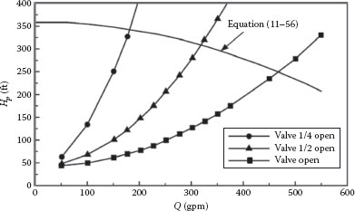
FIGURE E11.1 Flow range with linear trim.
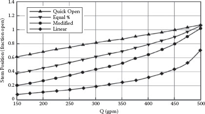
FIGURE E11.2 Flow rate versus stem position for various trim functions.
The Q versus X relation for various valve trim functions can be determined as follows. First, a flow rate (Q) is assumed, which is used to calculate the Reynolds number and hence the pipe friction factor and the loss coefficients for the pipe and fittings. Then a valve trim characteristic function is assumed and, using the pump head function parameters, the right-hand side of Equation 11.57 is evaluated. This gives the value for f(X) for that trim, which corresponds to the assumed flow rate. This is then equated to the appropriate trim function for the valve given above (e.g., EP, MP, L, QO), and the resulting equation is solved for X (this may require an iteration procedure or the use of a nonlinear equation solver). The procedure is repeated over a range of assumed Q values for each of the given trim functions, giving the Q versus X response for each trim as shown in Figure E11.2. Aside from the quick open response, it is evident that the equal percentage trim results in the most linear response and also results in the greatest range or “turndown” (which is inversely proportional to the slope of the line).
In addition to the ISA/ANSI standards and the manufacturers’ handbooks (e.g., Emerson/Fisher), there are numerous other references that offer guidelines and practical tips for selecting a suitable control valve for a specific application (e.g., Driskill et al. 1969, 1970, Christy 1996, Singleton 2013, etc.).
The following are the most significant points covered in this chapter:
Safety relief valves
• The isentropic nozzle as the theoretical basis for sizing an SRV, and how it differs from the actual valve geometry
• The three elements needed to size an SRV for a given mass relief flow rate
• The equations and data needed to size an SRV for liquids, ideal gases, two-phase (or any) fluids, as well as flashing equilibrium and nonequilibrium flows using the HDI and HNDI methods.
• Selection of the proper discharge coefficient
Control valves
• The function of a control valve and the various trim characteristics
• The orifice equation as the theoretical basis for sizing control valves
• The valve sizing coefficient, and the various correction factors for attached piping, the flow coefficient, flashing and cavitating liquids, viscous liquids.
• Equations for subsonic and choked gas flow.
• General numerical (HDI) method for two-phase or any flow regime
• How to match the control valve trim to the piping system characteristics
SAFETY RELIEF VALVES
1. Rework Example 11.1 using the HDI method and tables for the properties of air, and compare the results with the example. Which answer do you think is the best, and why? (You should have access to a computer database file for the thermodynamic properties of various gases and vapors.)
2. An SRV must be sized to relieve hot water from a water heater at a rate of 20 lbm/s. If the water is at 220°F and 45 psia, what nozzle area would be required? For the valve, KDL = 0.65 and KDg = 0.98.
CONTROL VALVES
3. Air at 100 psia and 60°F is being controlled through a venturi control valve. The backpressure at the valve discharge is P2 = 30 psia. The flow rate through the valve at its maximum opening is to be found, using the equations from ISA-75.01.01 and numerical integration. The parameters provided by the valve company for a wide-open valve are C1 = 14.1 and XT = 0.1254 (the low value of XT indicates that it is a high-recovery valve). Additionally, Fγ = 1.0 (value for air); Cγ = 355.9 (value for air); molecular weight for air = 29; ideal gas compressibility Z = 1.0; and specific heat ratio, γ = 1.4 calculated at the inlet pressure and temperature.
4. You want to control the flow rate of a liquid in a transfer line at 350 gpm. The pump in the line has the characteristics shown in Figure 8.2, with a 5 1/4 in. impeller. The line contains 150 ft of 3 in. sch 40 pipe, 10 flanged elbows, four gate valves, and a 3 × 3 control valve. The pressure and elevation at the entrance and exit of the line are the same. The valve has an equal percentage trim. What should the value of Cv be for the valve to achieve the desired flow rate? The fluid has a viscosity of 5 cP and an SG of 0.85.
5. A liquid with a viscosity of 25 cP and an SG of 0.87 is pumped from an open tank to another tank in which the pressure is 15 psig. The line is 2 in. sch 40 diameter, 200 ft long, and contains eight flanged elbows, two gate valves, a control valve, and an orifice meter.
What should be the diameter of the orifice in the line for a flow rate of 100 gpm, if the pressure across the orifice is not to exceed 80 in. H2O?
6. Water at 60°F is to be transferred at a rate of 250 gpm from the bottom of a storage tank to the bottom of a process vessel. The water level in the storage tank is 5 ft above ground level, and the pressure in the tank is 10 psig. In the process vessel, the level is 15 ft above ground and the pressure is 20 psig. The transfer line is 150 ft of 3 in. sch 40 pipe, containing eight flanged elbows, three 80% reduced trim gate valves, and a 3 × 3 control valve. The pump in the line has the same characteristics as those shown in Figure 8.2 with an 8 in. impeller, and the control valve has a linear characteristic. If the stem on the control valve is set to provide the desired flow rate under the specified conditions, what should be the required value of the valve coefficient to achieve this?
7. A piping system takes water at 60°F from a tank at atmospheric pressure to a plant vessel at 25 psig that is 30 ft higher than the upstream tank. The transfer line contains 300 ft of 3 in. sch 40 pipe, 10 90° elbows, an orifice meter, a 2 × 3 pump with a 7 3/4 in. impeller (with the characteristic as given on Figure 8.2), and a 3 × 2 equal percentage control valve. A constant flow rate of 200 gpm is required in the system.
(a) What size orifice should be installed if the DP (differential pressure) cell used to measure the pressure drop across the orifice has a maximum range of 25 in. H2O?
(b) What is the Cv of the valve that gives the required flow rate?
A |
Flow cross-sectional area, [L2] |
Ao |
Theoretical flow area for control valve, [—] |
AoKd |
Effective flow area for fully open control valve, [L2] |
cp |
Specific heat at constant pressure, [FL/M] |
cv |
Specific heat at constant volume, [FL/M] |
C1 |
Cg/Cv, [M/L7]1/2 |
C2 |
Correction factor for isentropic exponent, Equation 11.40 [—] |
Cd |
Control valve discharge coefficient , [—] |
Cg |
Flow correction factor for gases [—] |
Co |
Flow coefficient for control valve (= Kd), [—] |
Cv |
Control valve sizing coefficient, [L7/M]1/2 |
Cv |
Control valve viscosity correction coefficient, Figure 11–12 [—] |
d |
Control valve nominal valve size, [L] |
EP |
Equal percentage control valve trim, [—] |
Fd |
Control valve style modifier, [—] |
FF |
Control valve liquid critical pressure ratio (= rc), [—] |
FG |
Vena contracta correction for gas flow, Equations 11.35, [—] |
FL |
Control valve liquid pressure recovery factor (= Km)½, [—] |
Fp |
Control valve piping geometry factor, [—] |
Fv |
Control valve viscosity correction factor, [—] |
Gc |
Maximum (choked) mass flux, [M/L2t] |
Gn |
Measured mass flux through actual nozzle, [M/L2t] |
Go |
Theoretical mass flux through isentropic nozzle, [M/tL2] |
hv |
Head loss in ft of fluid, [L] |
H |
Specific enthalpy (per unit mass), [L2/t2] |
Hp |
Pump head, [L] |
Hs |
System head (Figure 11.14), [L] |
k |
Isentropic exponent = γ (ideal gas), [—] |
Kd |
Flow coefficient for control valve (= Co), [—] |
KD |
SRV discharge coefficient, [—] |
Kf |
Friction loss coefficient (pipe, fittings, etc.), [—] |
KDG |
SRV gas discharge coefficient, [—] |
KDL |
SRV liquid discharge coefficient, [—] |
Km |
Control valve liquid recovery coefficient , [—] |
Kv |
Viscosity correction factor, Equation 11.7, [—] |
L |
Linear control valve trim, [—] |
L |
Nozzle length, [L] |
ṁ |
Mass flow rate, [M/t] |
MP |
Modified equal percentage control valve trim, [—] |
Mw |
Molecular weight, [M/mol] |
NRev |
Control valve Reynolds number, [—] |
N |
“Equation constant” for unit conversions, [—] |
P |
Pressure, [F/L2] |
Pb |
Back pressure on valve, [F/L2] |
ΔPcav |
Pressure at which cavitation appears, [F/L2] |
Pc |
Critical (choked) pressure, [F/L2] |
Ptc |
Thermodynamic critical pressure (absolute), [F/L2] |
Pv |
Fluid vapor pressure, [F/L2] |
Q |
Volumetric flow rate, gpm, [L3/t] |
QO |
Quick opening control valve trim, [—] |
R |
Ideal gas constant, [ML2/mol t2 °] |
rc |
Critical pressure ratio at which choking will occur (= P2c/Pv = FF), [—] |
S |
Slip, ratio of gas velocity to liquid velocity in a mixture, [—] |
SRV |
Safety relief valve |
T |
Absolute temperature, [°] |
u |
Velocity, [L/t] |
x |
Quality, or mass fraction of gas/vapor in mixture, [—] |
X |
Fraction of fully open stem for control valve, [—] |
X |
Dimensionless pressure crop across control valve, Equation 11.43, [—] |
XT |
Maximum value of X for a specific valve, [—] |
xT |
Control valve pressure differential ratio factor without fittings at choked flow, [—] |
Y |
Control valve expansion factor, [—] |
GREEK
α |
Volume fraction of gas/vapor in mixture, [—] |
β |
Dn/Dp = do/D, Ratio of nozzle or orifice diameter to inlet pipe diameter, [—] |
γ |
Cp/Cv = k, [—] |
ν |
Specific volume, [L3/M] |
ρ |
Density, [M/L3] |
SUBSCRIPTS
b |
Valve exit |
c |
Critical or choked value |
e |
Equilibrium |
G |
Gas/vapor |
L |
Liquid |
n |
Nozzle exit |
o |
Nozzle entrance |
s |
Saturation |
vc |
Vena contracta |
Baumann, H.D., Control Valve Primer, Instrument Society of America, Durham, NC, 1991.
Cheremisinoff, N.P. and P.N. Cheremisinoff, Instrumentation for Process Flow Engineering, Technomic Publishing Company, Lancaster, PA, 1987.
Center for Chemical Process Safety (CCPS), Guidelines for Pressure Relief and Effluent Handling Systems, American Institute of Chemical Engineers, New York (1998) (in revision).
Christy, J.R.E., On selecting appropriate control valves for pipework systems, Chemical Engineering Education, Winter 1996, pp. 54–57.
Darby, R., Control valves: Match the trim to the selection, Chem. Eng., 104, 147–152, June 1997.
Darby, R and K Molavi, “Viscosity Correction Factor for Safety Relief Valves”, Process Safety Progress, 16(2), 80–83, 16, no.2 (1997)
Darby, R., F.E. Self, and V.H. Edwards, Properly size pressure-relief valves for two-phase flow, Chem. Eng., 109(6), 68–74, June 2002.
Darby, R., On two-phase frozen and flashing flows in safety relief valves, J. Loss Prev. Process Ind., 17, 255–259, 2004.
Darby, R., Size safety-relief valves for any conditions, Chem. Eng., 112(9), 42–50, September 2005.
Darby, R., A Review of the HDI/HNDI Valve Sizing Method and Appropriate Discharge Coefficient, DIERS Users Group, Reno, NV, October 2010.
Driskell, L.R., New approach to control valve sizing, Hydrocarb. Process., 48(7), 131–134, July 1969.
Driskell, L.R., Sizing valves for gas flow, ISA Trans., 9(4), 325–331, 1970. (Note: Both Driskell papers define AK = Cv FL/38 where K is the “flow coefficient including velocity of approach”.)
Emerson Process Management, Fisher Controls, Control Valve Handbook, 4th edn., Emerson Process Management, Marshalltown, IA, 2005.
Fisher Controls, Catalog 10, Ch. 2, Marshalltown, IA, 1987.
Fisher Controls, Control Valve Source Book, Fisher Controls, International, Marshalltown, IA, 1990.
Henry, R.E. and H.K. Fauske, The two-phase critical flow of one-component mixtures in nozzles, orifices and short tubes, Trans. Am. Soc. Mech. Eng., J. Heat Transfer, 93, 179–187, May 1971.
Hutchison, J.W., ISA Handbook of Control Valves, 1st edn., Instrument Society of America, Durham, NC, 1971.
International Electrotechnical Commission (IEC), IEC-60534-2-1. Industrial Process Control Valves—Part 2-1: Flow Capacity—Sizing Equations for Fluid Flow under Installed Conditions, 2011.
Instrument Society of America (ISA), ISA-75.01.01 (60534-2-1 MOD). Industrial Process-Control Valves—Part 2–1: Flow Capacity—Sizing Equations for Fluid Flow under Installed Conditions, 2012.
Lenzing, F., J. Friedel, J. Cremers, and M. Alhusein, Prediction of the maximum full lift safety valve two-phase flow capacity, J. Loss Prev. Proc. Ind., 11, 307–321, 1998.
Lenzing, T., J. Schecker, L. Friedel, and J. Cremers, Safety relief valve critical mass flux as a function of fluid properties and valve geometry, Presented at ISO TC 185 WG1 Meeting, Paper N103, Rome, Italy, October 29–31 1997.
Lipták, B.G., C.G. Langford, F.M. Cain, and H.D. Baumann, Sizing, Chapter 16, in Process Control and Optimization, vol. 2 of Instrument Engineers’ Handbook, 4th edn., B.G. Liptaak, (Ed.), CRC Press, Boca Raton, FL, 2006, p. 1234
NIST (National Institute of Science and Technology), Standard Reference Database 23, Reference Fluid Thermodynamic and Transport Properties—REFPROP, Version 8.0 (and subsequent versions), 2015.
Singleton, E., A Specifier’s Guide to Control Valves, KCI Publishing, 2013.
Stiles, G.F., Liquid viscosity effects on control valve sizing, 14th Annual Symposium on Instrumentation for the Process Industries, Texas A&M University, College Station, TX 1964.