9	Compressible Flows

“Surely it is not knowledge, but learning; not owning but earning; not being there, but getting there; that gives us the greatest pleasure.”

—Carl Friedrich Gauss, 1777–1855, Mathematician and Physicist

I.    GAS PROPERTIES

The main difference between the flow behavior of incompressible and compressible fluids, and the equations that govern them, is the effect of variable density, for example, the dependence of density upon pressure and temperature. At low velocities (relative to the speed of sound), relative changes in pressure and associated effects on density are often small and the assumption of incompressible flow with a constant (average) density may be reasonable. It is when the gas velocity approaches the speed at which a pressure wave propagates (i.e., the speed of sound) that the effects of compressibility become the most significant. It is this condition of high-speed gas flow (“fast gas”) that is of greatest concern to us here.

A.    IDEAL GAS

All gases are “nonideal” in that there are conditions under which the density of the gas may not be accurately represented by the ideal gas law:

$\text{ρ}=\frac{PM}{RT}$

(9.1)

However, there are also conditions under which this law provides a very good representation of the density for virtually any gas. In general, the higher the temperature and the lower the pressure relative to the critical temperature and pressure of the gas, the better the ideal gas law represents gas properties. For example, the critical conditions for CO₂ are 304 K, 72.9 atm, whereas for N₂ they are 126 K, 33.5 atm. Thus, at normal atmospheric conditions (300 K, 1 atm), N₂ can be described very accurately by the ideal gas law, whereas CO₂ deviates significantly from this law under such conditions. This is readily discernible from the P–H diagrams for the substance (see, e.g., Appendix D), because ideal gas behavior can be identified with the conditions under which the enthalpy is independent of pressure, that is, the constant temperature lines on the P–H diagram are vertical (see Section III.B of Chapter 5). For the most common gases (e.g., air) at conditions that are not extreme, the ideal gas law provides quite an acceptable representation for most engineering purposes. For gases/vapors and two-phase flows, a thermodynamic database for the fluid properties is generally required for calculations (e.g., NIST–REFPROP Database 23, v. 9.1, 2015).

We will consider the flow behavior of gases under two possible conditions: isothermal and isentropic (or adiabatic). The isothermal (constant temperature) condition may be approximated, for example, in a long pipeline in which the residence time of the gas is long enough that there is plenty of time to reach thermal equilibrium with the surroundings. Under these conditions for an ideal gas, Equation 9.1 implies

$\frac{P}{\text{ρ}}=\text{Constant}=\frac{P_1}{{\text{ρ}}_1}=\frac{P_2}{{\text{ρ}}_2},\text{etc}.$

(9.2)

The adiabatic condition occurs, for example, when the residence time of the fluid is short, as for flow through a short pipe, valve, orifice, etc. and/or for well-insulated boundaries. When friction loss is small, the system can also be described as locally isentropic. It can readily be shown that an ideal gas under isentropic conditions obeys the relationship:

$\frac{P}{{\text{ρ}}^k}=\text{Constant}=\frac{P_1}{{\text{ρ}}_1^k}=\frac{P_2}{{\text{ρ}}_2^k},\text{etc}.$

(9.3)

where k = c_p/c_v is the “isentropic exponent” and, for an ideal gas, c_p = c_v + R/M. For diatomic gases, k ≈ 1.4, whereas for triatomic and higher gases, k ≈ 1.3. Equation 9.3 is also often used for nonideal gases, with k as a variable. A table of properties of various gases, including the isentropic exponent, is given in Appendix C, which also includes a plot of k as a function of temperature and pressure for non-ideal steam.

B.    THE SPEED OF SOUND

Sound is a small amplitude compression pressure wave, and the speed of sound is the velocity at which this wave will travel through a medium. An expression for the speed of sound can be derived as follows. With reference to Figure 9.1, we consider a sound wave moving from left to right with velocity c. If we take the wave as our reference system, this is equivalent to considering a standing wave with the medium moving from right to left with velocity c. Since the conditions are different upstream and downstream of the wave, we represent these differences by ΔV, ΔT, ΔP, and Δρ. The conservation of mass principle applied to the flow through the wave reduces to:

$\dot{m}=\text{ρ}Ac=\left(\text{ρ}+\Delta \text{ρ}\right)A\left(c-\Delta V\right)$

(9.4)

or

$\text{Δ}V=c\frac{\Delta \text{ρ}}{\text{ρ}+\text{Δρ}}$

(9.5)

Likewise, a momentum balance on the fluid “passing through” the wave is

${\displaystyle \sum F=\dot{m}\left(V_2-V_1\right)}$

(9.6)

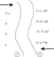
FIGURE 9.1 Sound wave moving at velocity c.

which becomes, in terms of the parameters in Figure 9.1,

$PA-\left(P+\Delta P\right)A=\text{ρ}Ac\left(c-\Delta V-c\right)$

(9.7)

or

$\text{Δ}P=\text{ρ}c\text{Δ}V$

(9.8)

Eliminating ΔV from Equations 9.5 and 9.8 and solving for c² gives

$c^2=\frac{\Delta P}{\Delta \text{ρ}}\left(1+\frac{\Delta \text{ρ}}{\text{ρ}}\right)$

(9.9)

For an infinitesimal wave under isentropic conditions, the term (1 + Δρ/ρ) ≈ 1, so that Equation 9.9 becomes:

$c={\left[{\left(\frac{\partial P}{\partial \text{ρ}}\right)}_s\right]}^{1/2}={\left[k{\left(\frac{\partial P}{\partial \text{ρ}}\right)}_T\right]}^{1/2}$

(9.10)

where the equivalence of the terms in the two radicals follows from Equations 9.2 and 9.3.

For an ideal gas, Equation 9.10 reduces to:

$c={\left(\frac{kP}{\text{ρ}}\right)}^{1/2}={\left(\frac{kRT}{M}\right)}^{1/2}$

(9.11)

For solids and liquids:

${\left(\frac{\partial P}{\partial \text{ρ}}\right)}_s=\frac{K}{\text{ρ}}$

(9.12)

where K is the bulk modulus (or “compressive stiffness”) of the material. It is evident that the speed of sound in a completely incompressible medium would be infinite. From Equation 9.11, we see that the speed of sound in an ideal gas is determined entirely by the nature of the gas (M and k) and the temperature (T).

II.    PIPE FLOW

Consider a gas in steady flow in a uniform (constant cross section) pipe. The mass flow rate and mass flux (G) are the same at all locations along the pipe:

$G=\frac{\dot{m}}{A}=\text{ρ}V=\text{Constant}$

(9.13)

Now the pressure drops along the pipe because of energy dissipation (e.g., friction), just as for an incompressible fluid. However, because the density decreases with decreasing pressure and the product of the density and velocity must be constant, the velocity must increase as the gas moves through the pipe. This increase in velocity corresponds to an increase in kinetic energy per unit mass of gas, which also results in a drop in temperature. There is a limit as to how high the velocity can get in a straight pipe, however, which we will discuss shortly.

Because the fluid velocity and properties change from point to point along the pipe, in order to analyze the flow we apply the differential form of the Bernoulli equation to a differential length of pipe (dL):

$\frac{dP}{\text{ρ}}+gdz+d\left(\frac{V^2}{2}\right)+\delta e_f+\delta w=0$

(9.14)

If there is no shaft work done on the fluid in this system and the elevation (potential energy) change can be neglected, Equation 9.14 can be rewritten using Equation 9.13 as follows:

$\frac{dP}{\text{ρ}}+\frac{G^2}{\text{ρ}}d\left(\frac{1}{\text{ρ}}\right)=-\text{δ}{e}_f=-\frac{2f{V}^{2}dL}{D}=-\frac{2f}{D}{\left(\frac{G}{\text{ρ}}\right)}^{2}dL$

(9.15)

where the friction factor f is a function of the Reynolds number:

$f=\text{fn}\left(N_{Re}=\frac{DG}{\text{μ}}~\text{constant}\right)$

(9.16)

Because the gas viscosity is not highly sensitive to pressure, for isothermal flow the Reynolds number and hence the friction factor will be very nearly constant along the pipe. For adiabatic flow, the viscosity may change as the temperature changes, but these changes are usually small. Equation 9.15 is thus valid for any prescribed conditions, and we will apply it to an ideal gas in both isothermal and adiabatic (isentropic) flow.

A.    ISOTHERMAL FLOW

Substituting Equation 9.1 for the density into Equation 9.15, rearranging and integrating from the inlet of the pipe (point 1) to the outlet (point 2), and solving the result for G gives

$\begin{array}{l}G={\left[\frac{M\left(P_1^2-P_2^2\right)/\left(2RT\right)}{2fL/D+\ln \left(P_1/P_2\right)}\right]}^{1/2}\hfill \\ =\sqrt{P_1{\text{ρ}}_1}{\left[\frac{1-P_2^2/P_1^2}{4fL/D-2\ln \left(P_2/P_1\right)}\right]}^{1/2}\hfill \end{array}$

(9.17)

If the logarithmic term in the denominator (which comes from the change in kinetic energy of the gas) is neglected, the resulting equation is called the Weymouth equation. Furthermore, if the average density of the gas is used in the Weymouth equation, that is,

$\overline{\rho }\text{=}\frac{\left(P_1+P_2\right)M}{2RT}\text{or}\frac{M}{2RT}=\frac{\overline{\rho }}{P_1+P_2}$

(9.18)

Equation 9.17 reduces identically to the Bernoulli equation for an incompressible fluid in a straight, uniform pipe, which can be written in the form

$G={\left(\frac{\overline{\rho }\left(P_1-P_2\right)}{2fL\text{/}D}\right)}^{1/2}=\sqrt{P_1\overline{\rho }}{\left(\frac{1-P_2/P_1}{2fL/D}\right)}^{1/2}$

(9.19)

Inspection of Equation 9.17 shows that as P₂ decreases, both the numerator and denominator increase, with opposing effects. By setting the derivative of Equation 9.17 with respect to P₂ (i.e., dG/dP₂) equal to zero, the value of P₂ that maximizes G and the corresponding expression for the maximum G can be found. If the conditions at this state (i.e., the maximum mass flux) are denoted by an asterisk (e.g., $P_2^{\ast }$, G*), the result is

$G*=P_2^{\ast }\sqrt{\frac{M}{RT}}=P_2^{\ast }\sqrt{\frac{{\text{ρ}}_1}{P_1}}$

(9.20)

or

$V_2^{\ast }=\sqrt{\frac{RT}{M}}=\sqrt{\frac{P_1}{{\text{ρ}}_1}}=c$

(9.21)

That is, as P₂ decreases, the mass velocity in the conduit will increase up to a maximum value of G*, at which point the velocity at the end of the pipe reaches the speed of sound. Any further reduction in the downstream pressure (P₂) can have no effect on the flow in the pipe, because the speed at which pressure change information can be transmitted is the speed of sound. That is, since pressure changes are transmitted at the speed of sound, they cannot propagate upstream in a gas that is already traveling at the speed of sound. Therefore, the pressure inside the downstream end of the pipe will remain at $P_2^{*}$ regardless of how low the pressure outside the end of the pipe (P₂) may fall. This condition is called choked flow and is a very important concept because it establishes the conditions under which maximum gas flow can occur in a conduit. When the flow becomes choked, the mass flow rate in the pipe will be insensitive to the value of the exit pressure (but will still be dependent upon the upstream conditions).

Although Equation 9.17 appears to be explicit for G, it is actually implicit because the friction factor depends upon the Reynolds number, which depends on G. However, the Reynolds number under choked flow conditions is often high enough that fully turbulent flow prevails, in which case the friction factor depends only on the relative pipe roughness ε/D, i.e., (Equation 6.40):

$\frac{1}{\sqrt{f}}=-4\log \left(\frac{\text{ε/}D}{3.7}\right)$

(9.22)

If the upstream pressure and flow rate are known, the downstream pressure (P₂) can be found by rearranging Equation 9.17, as follows:

$\frac{P_2}{P_1}={\left\{1-\frac{G^2}{P_1{\text{ρ}}_1}\left[\frac{4fL}{D}-2\ln \left(\frac{P_2}{P_1}\right)\right]\right\}}^{1/2}$

(9.23)

which is implicit in P₂. A first estimate for P₂ can be obtained by neglecting the logarithmic term on the right (the result corresponding to the Weymouth approximation). This first estimate can then be inserted into the last term in Equation 9.23 to provide a second estimate for P₂, and the process can be repeated as necessary. Alternately, a spreadsheet can be used with the “solve” or “goal seek” function to solve the equation.

Equation 9.23 can be also rewritten in another form in terms of the Mach number, N_Ma = V/c. From Equations 9.13 and 9.21, $G=\text{ρ}V=\text{ρ}c{N}_{Ma}=\sqrt{P\text{ρ}}{N}_{Ma}=\text{const}$ and, in combination with Equation 9.2, we have PN_Ma = const for isothermal flow. Thus, with Equation 9.23, we have

$\frac{P_2}{P_1}=\frac{N_{Ma1}}{N_{Ma2}}={\left\{1-N_{Ma1}^2\left[\frac{4fL}{D}-2\ln \left(\frac{N_{Ma1}}{N_{Ma2}}\right)\right]\right\}}^{1/2}$

(9.24)

or

$\frac{4fL}{D}=\frac{1}{N_{Ma1}^2}-\frac{1}{N_{Ma2}^2}+2\ln \left(\frac{N_{Ma1}}{N_{Ma2}}\right)$

(9.25)

B.    ADIABATIC FLOW

In the case of adiabatic flow, we can use Equations 9.1 and 9.3 to eliminate density and temperature from Equation 9.15. This can be called the locally isentropic approach, because the friction loss is still included in the energy balance. Actual flow conditions are often somewhere between isothermal and adiabatic, in which case the flow behavior can be described by the isentropic equations, with the isentropic constant k replaced by a “polytropic” constant (or “isentropic exponent”) γ, where 1 < γ < k, as is done for compressors (the isothermal condition corresponds to γ = 1, whereas truly isentropic flow corresponds to γ = k). This same approach can be used for some nonideal gases by using a variable isentropic exponent for k (e.g., for steam, see Figure C.1).

Combining Equations 9.1 and 9.3 leads to the following expressions for density and temperature as a function of pressure:

$\text{ρ}={\text{ρ}}_1{\left(\frac{P}{P_1}\right)}^{1/k},T=T_1{\left(\frac{P}{P_1}\right)}^{\left(k-1\right)/k}$

(9.26)

Using these expressions to eliminate ρ and T from Equation 9.15 and solving for G gives

$G=\sqrt{P_1{\text{ρ}}_1}{\left[\frac{2\left(\frac{k}{k+1}\right)\left(1-{\left(\frac{P_2}{P_1}\right)}^{\left(k+1\right)/k}\right)}{\frac{4fL}{D}-\frac{2}{k}\ln \left(\frac{P_2}{P_1}\right)}\right]}^{1/2}$

(9.27)

If the system contains fittings as well as straight pipe, the term 4fL/D (= K_{f pipe}) can be replaced by ΣK_f, that is, the sum of all loss coefficients in the system.

Just as for isothermal flow, Equation 9.27 can be rewritten in terms of Mach number, as follows. From Equations 9.13 and 9.11, $G=\text{ρ}V=\text{ρ}c{N}_{Ma}=\sqrt{kP\text{ρ}}{N}_{Ma}=\text{const}$. In combination with Equation 9.3, this gives P^{(k + 1)/(2k)} N_Ma = const, and

$\frac{P_2}{P_1}={\left(\frac{N_{Ma1}}{N_{Ma2}}\right)}^{2k/\left(k+1\right)}$

(9.28)

so that (9.27) can be rewritten in the form:

$N_{Ma1}={\left[\frac{\left(\frac{2}{k+1}\right)\left(1-{\left(\frac{N_{Ma1}}{N_{Ma2}}\right)}^2\right)}{\frac{4fL}{D}-\frac{4}{k+1}\ln \left(\frac{N_{Ma1}}{N_{Ma2}}\right)}\right]}^{1/2}$

(9.29)

or

$\frac{4fL}{D}=\frac{2}{k+1}\left[\frac{1}{N_{Ma1}^2}-\frac{1}{N_{Ma2}^2}+2\ln \left(\frac{N_{Ma1}}{N_{Ma2}}\right)\right]$

(9.30)

C.    CHOKED FLOW

For isentropic flow (just as for isothermal flow), as the downstream pressure drops, the mass velocity increases until it reaches a maximum. When the downstream pressure reaches the point where the velocity becomes sonic at the end of the pipe, the flow is choked. This can be shown by differentiating Equation 9.27 with respect to P₂ (as before) or alternatively as follows, noting that G = ṁ/A = ρV:

$\frac{\partial G}{\partial P}=\frac{\partial \left(\text{ρ}V\right)}{\partial P}=\text{ρ}\frac{\partial V}{\partial P}+V\frac{\partial \text{ρ}}{\partial P}=0\left(\text{for}\max G\right)$

(9.31)

For isentropic conditions, the differential form of the Bernoulli equation is

$\frac{dP}{\text{ρ}}+VdV=0\text{or}\frac{\partial V}{\partial P}=-\frac{1}{\text{ρ}V}$

(9.32)

Substituting this into Equation 9.31 gives

$-\frac{1}{V}+V\frac{\partial \text{ρ}}{\partial P}=0$

(9.33)

However, it is noted that

$c^2={\left(\frac{\partial P}{\partial \text{ρ}}\right)}_s$

(9.34)

so that Equation 9.33 can be written as:

$-\frac{1}{V}+\frac{V}{c^2}=0\text{or}V=c$

(9.35)

This shows that when the mass velocity reaches a maximum, the velocity is sonic (i.e., the flow is choked).

1.  Isothermal

Under isothermal conditions, choked flow occurs when:

$V_2=c=V_2^{*}=\sqrt{\frac{RT}{M}}=\sqrt{\frac{P_1}{{\text{ρ}}_1}}$

(9.36)

where the asterisk denotes the sonic state. Thus:

$G*={\text{ρ}}_2{V}_2^{*}=\frac{P_2^{*}M}{RT}\sqrt{\frac{RT}{M}}=\sqrt{P_1{\text{ρ}}_1}\frac{P_2^{*}}{P_1}$

(9.37)

If G* is eliminated from Equations 9.17 and 9.37, the result can be solved for ΣK_f, to give:

$\begin{array}{|c|}\hline {\displaystyle \sum K_f}={\left(\frac{P_1}{P_2^{*}}\right)}^2-2\ln \left(\frac{P_1}{P_2^{*}}\right)-1\\ \hline\end{array}$

(9.38)

where 4fL/D in Equation 9.17 has been replaced by ΣK_f. Equation 9.38 shows that the pressure at the inside of the end of the pipe at which the flow becomes sonic $\left(P_2^{*}\right)$ is a unique function of the upstream pressure (P₁) and the sum of the loss coefficients in the system (ΣK_f). Since Equation 9.38 is implicit in $P_2^{*}$, it must be solved for $P_2^{*}$ by iteration for given values of ΣK_f, and P₁, or on a spreadsheet using the “solve” or “goal seek” function. Equation 9.38 thus enables the determination of the choke pressure, $P_2^{*}$, as a function of ΣK_f, and P₁.

2.  Adiabatic

For adiabatic (or locally isentropic) conditions, the corresponding expressions are

$\begin{array}{cc}{V}_2=c=V_2^{*}={\left(\frac{kR{T}_2}{M}\right)}^{1/2},& \frac{T_2}{T_1}\end{array}={\left(\frac{P_2}{P_1}\right)}^{\left(k-1\right)/k}$

(9.39)

and

$G*=\frac{P_2^{*}M}{R{T}_2^{*}}{\left(\frac{kR{T}_2^{*}}{M}\right)}^{1/2}=\sqrt{P_1{\text{ρ}}_1}{\left[k{\left(\frac{P_2^{*}}{P_1}\right)}^{\left(k+1\right)/k}\right]}^{1/2}$

(9.40)

Eliminating G* from Equations 9.27 and 9.40 and solving for ΣK_f gives

$\begin{array}{|c|}\hline {\displaystyle \sum K_f}=\frac{2}{k+1}\left[{\left(\frac{P_1}{P_2^{*}}\right)}^{\left(k+1\right)/k}-1\right]-\frac{2}{k}\ln \left(\frac{P_1}{P_2^{*}}\right)\\ \hline\end{array}$

(9.41)

Just as for isothermal flow, this is an implicit expression for the “choke pressure”$\left(P_2^{*}\right)$ as a function of the upstream pressure (P₁), the loss coefficients (ΣK_f), and the isentropic exponent (k), which is most easily solved by iteration using a spreadsheet. It is very important to realize that once the pressure at the end of the pipe falls to $P_2^{*}$ and choked flow occurs, all of the conditions within the pipe ($G=G*,P_2=P_2^{*}$, etc.) will remain the same regardless of how low the pressure outside the end of the pipe falls. The pressure drop within the pipe (which determines the flow rate) is always $P_1-P_2^{*}$ when the flow is choked.

D.    THE EXPANSION FACTOR

The adiabatic flow equation (Equation 9.27) can be represented in a more convenient form as

$G=Y{\left(\frac{2{\text{ρ}}_1\text{Δ}P}{{\displaystyle \sum K_f}}\right)}^{1/2}=Y\sqrt{P_1{\text{ρ}}_1}{\left[\frac{2\left(1-P_2/P_1\right)}{{\displaystyle \sum K_f}}\right]}^{1/2}$

(9.42)

where

ρ₁ = P₁M/RT₁

ΔP = P₁ − P₂

Y is the expansion factor

Note that Equation 9.42 without the Y term is the Bernoulli equation for an incompressible fluid of density ρ₁. Thus, the expansion factor is simply the ratio of the adiabatic mass flux (Equation 9.27) to the corresponding incompressible mass flux (Y = G_adiabatic/G_{incompressible}) and is a unique function of P₂/P₁, k, and K_f. For convenience, values of Y are shown in Figure 9.2a for k = 1.3 and Figure 9.2b for k = 1.4, as a function of ΔP/P₁ and ΣK_f (which is denoted simply by K on these plots) (Crane, 1991). The conditions corresponding to the lower ends of the lines on the plots (i.e., the “button”) represent the sonic (choked flow) state where $P_2=P_2^{*}$. These same conditions are given in the table accompanying the plots, which enable the relationships for choked flow to be determined more precisely than is possible from reading the plots. Note that it is not possible to extrapolate beyond the “button” at the end of the lines in Figure 9.2a and b because this represents the choked flow state, in which $P_2=P_2^{*}$ (inside the pipe) and is independent of the external exit pressure.

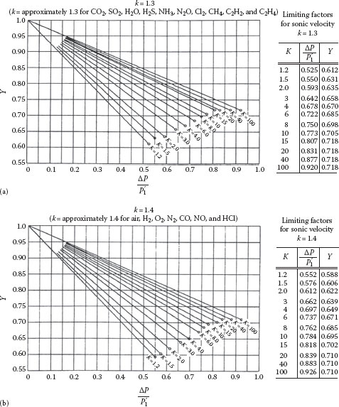
FIGURE 9.2 Expansion factor for adiabatic flow in piping systems. (a) k = 1.3 and (b) k = 1.4. (From Crane, C., Flow of fluids through valves, fittings and pipe, Technical Manual 410, Crane Co., New York, 1991 [and subsequent issues].)

Figure 9.2 provides a convenient way of solving compressible adiabatic flow problems for piping systems. Some iteration is normally required, because the value of K_f depends upon the Reynolds number, which cannot be determined until G is found. An example of the procedure for solving a typical problem is as follows.

E.    FRICTIONLESS ADIABATIC FLOW

The adiabatic flow of an ideal gas flowing through a frictionless conduit or a constriction (such as an orifice, nozzle, or valve) can be analyzed as follows. The total energy balance is

$\Delta h+g\Delta z+\frac{1}{2}\Delta V^2=q+w$

(9.43)

For horizontal adiabatic flow with no external work, this becomes

$\Delta h+\frac{1}{2}\Delta V^2=0$

(9.44)

where

$\Delta h=\Delta \left(c_{p}T\right)=\frac{k}{k-1}\Delta \left(\frac{P}{\text{ρ}}\right)$

(9.45)

This follows from the ideal gas relation c_p – c_v = R/M, and the definition of k (i.e., k = c_p/c_v). Equation 9.44 thus becomes

$\frac{k}{k-1}\left(\frac{P_2}{{\text{ρ}}_2}-\frac{P_1}{{\text{ρ}}_1}\right)+\frac{V_2^2-V_1^2}{2}=0$

(9.46)

Using the isentropic condition (P/ρ^k = constant) to eliminate ρ₂, this can be written as

$V_2^2-V_1^2=\frac{2k}{k-1}\left(\frac{P_1}{{\text{ρ}}_1}\right)\left[1-{\left(\frac{P_2}{P_1}\right)}^{\left(k-1\right)/k}\right]$

(9.47)

If V₁ is eliminated using the continuity equation, that is, (ρVA)₁ = (ρVA)₂, this becomes

$V_2={\left\{\frac{2k}{k-1}\left(\frac{P_1}{{\text{ρ}}_1}\right)\frac{\left[1-{\left(P_2/P_1\right)}^{\left(k-1\right)/k}\right]}{\left[1-{\left(A_2/A_1\right)}^2{\left(P_2/P_1\right)}^{2/k}\right]}\right\}}^{1/2}$

(9.48)

Now

$G=V_2{\text{ρ}}_2=V_2{\text{ρ}}_1{\left(\frac{P_2}{P_1}\right)}^{1/k}$

(9.49)

and assuming that the flow is from a larger conduit through a small constriction, such that A₁ ≫ A₂ (i.e., V₁ ≪ V₂), the term in the square brackets in the denominator of Equation 9.48 becomes equal to 1. Substituting the result into Equation 9.49 gives

$G=\sqrt{P_1{\text{ρ}}_1}{\left\{\frac{2k}{k-1}{\left(\frac{P_2}{P_1}\right)}^{2/k}\left[1-{\left(\frac{P_2}{P_1}\right)}^{\left(k-1\right)/k}\right]\right\}}^{1/2}$

(9.50)

Equation 9.50 represents flow through an “ideal nozzle,” that is, an isentropic constriction. Setting the derivative of Equation 9.50 to zero (i.e., ∂G/∂r = 0, where r = P₂/P₁), it can be shown that the mass flow is a maximum (choked) when

$\frac{P_2^{*}}{P_1}={\left(\frac{2}{k+1}\right)}^{k/\left(k-1\right)}$

(9.51)

For k = 1.4 (e.g., air), this has a value of 0.528. That is, if the downstream pressure is approximately one half or less of the upstream pressure, the flow will be choked. In such a case, the mass velocity can be determined by using Equation 9.40 with $P_2^{*}$ from Equation 9.51:

$G*=P_1{\left(\frac{2}{k+1}\right)}^{\left(k+1\right)/2\left(k-1\right)}\sqrt{\frac{kM}{R{T}_1}}=\sqrt{k{P}_1{\text{ρ}}_1}{\left(\frac{2}{k+1}\right)}^{\left(k+1\right)/2\left(k-1\right)}$

(9.52)

For k = 1.4, this reduces to

$G*=0.684P_1\sqrt{\frac{M}{R{T}_1}}=0.684\sqrt{P_1{\text{ρ}}_1}$

(9.53)

The mass flow rate under adiabatic conditions is always somewhat greater than that under isothermal conditions, but the difference is normally <20%. In fact, for long piping systems (L/D > 1000), the difference is usually less than 5% (see Figure 9.3).

It should be noted that the adiabatic equations reduce to the isothermal equations by setting k = 1. Also, the adiabatic equations can be applied to a nonideal gas by taking the parameter k to be a “polytropic exponent,” evaluated as an average value over the range of pressures considered.

The flow of compressible (as well as incompressible) fluids through nozzles and orifices will be considered in the following chapter on flow-measuring devices.

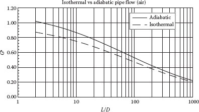
FIGURE 9.3 Dimensionless mass flux versus L/D for adiabatic and isothermal flow in a pipe. (From Holland and Bragg, 1995.)

F.    GENERAL FLUID PROPERTIES

The integrated form of the basic differential energy balance (Bernoulli) equation, Equation 9.14 (neglecting the potential energy and work terms), can be written between points 1 and 2 along the pipe and rearranged to solve for G²:

$G^2=\frac{-{\displaystyle {\int }_{P_1}^{P_2}\text{ρ}dP}}{\ln \left({\text{ρ}}_1{\text{/ρ}}_2\right)+\left({\displaystyle {\sum }_1^2{K}_{fi}+1}\right)/2}$

(9.54)

This expression is general and valid for any fluid (liquid, gas, ideal, nonideal, two-phase, etc.). It is only necessary to evaluate the integral of ρ versus P along the pipe to find the mass flux (and hence the mass flow rate). This can easily be done numerically on a spreadsheet, provided a fluid property (thermodynamic) database (such as NIST, 2015) is available to determine point values of ρ versus P over the proper interval, using the numerical approximation for the integral:

$-{\displaystyle \underset{P_1}{\overset{P_2}{\int }}\text{ρ}dP}\approx \frac{-1}{2}{\displaystyle \sum _{P_1}^{P_2}\left({\text{ρ}}_i+{\text{ρ}}_{i+1}\right)\left(P_i-P_{i+1}\right)}$

(9.55)

A suitable pressure interval [(i + 1) – i] is chosen (usually 1 psi), and Equations 9.54 and 9.55 are used to evaluate G versus P_i. The path to be followed over this pressure range should be adiabatic, which is approximated by an isentropic path, with the irreversible loss accounted for by the denominator in Equation 9.54. If the flow is choked, the value of G will exhibit a maximum before P_i reaches P₂, at which point the pressure is at the choke point inside the end of the pipe. If the pressure P₂ falls below that at the pipe exit before the maximum in G is reached, then the flow is not choked. This is actually an iterative process, as the loss coefficients (ΣK_f) depend on G through the Reynolds number. However, an initial estimate for these ΣK_f values can be taken as the fully turbulent values, which in many cases will suffice for all values of G of practical interest.

III.    GENERALIZED GAS FLOW EXPRESSIONS: IDEAL GAS

For adiabatic flow of an ideal gas in a constant area duct, the governing equations may be formulated in a more generalized dimensionless form that is useful for the solution of both subsonic and supersonic flows (the condition known as Fanno flow). We will present the resulting expressions and illustrate how to apply them here, but we will not show the derivation of all of them. For this, the reader is referred to publications such as that of Shapiro (1953) and Hall (1951) for the ideal gas and to Saad (1992), Cheng et al. (2012), Baltajiev (2012), Oosthuizen and Carscallen (2013), and Korelshteyn (2015) for the case of a general fluid.

A.    GOVERNING EQUATIONS

For steady flow of a gas at a constant mass flow rate in a uniform pipe, the pressure, temperature, velocity, density, etc. all vary from point to point along the pipe. The governing equations are the conservation of mass (continuity), conservation of energy, and conservation of momentum, all applied to a differential length of the pipe, as follows:

1.  Continuity

$\frac{\dot{m}}{A}=G=\text{ρ}V=\text{Constant}$

(9.56)

or

$\frac{d\text{ρ}}{\text{ρ}}+\frac{dV}{V}=0$

(9.57)

2.  Energy

$h+\frac{1}{2}{V}^2=\text{Constant}=h_o$

(9.58)

or

$dh+VdV=0$

(9.59)

Since the fluid properties are defined by the entropy and enthalpy, Equation 9.59 represents a curve on an h–s diagram, which is called a Fanno line.

3.  Momentum

$\frac{dP}{\text{ρ}}+VdV=-\frac{4{\text{τ}}_w}{\text{ρ}{D}_h}dL=-\frac{2f{V}^2}{D_h}dL$

(9.60)

By making use of the isentropic condition for an ideal gas (i.e., P/ρ^k = const.), the following relations can be obtained:

$h=c_{p}T=\frac{kRT}{\left(k-1\right)M}=\frac{P}{\text{ρ}}\left(\frac{k}{k-1}\right)$

(9.61)

$\frac{P}{\text{ρ}}=\frac{RT}{M}=\frac{c^2}{k}$

(9.62)

$N_{Ma}=\frac{V}{c}=\frac{G}{\sqrt{kP\text{ρ}}}$

(9.63)

where N_Ma is the Mach number.

The behavior of a nonideal gas (or any general homogeneous compressible Newtonian fluid) can be described by several dimensionless (positive) coefficients, or “isentropic exponents”, defined as follows:

$k_{P\text{ρ}}={\left(\frac{\partial \ln P}{\partial \ln \text{ρ}}\right)}_s$

(9.64)

$k_{TP}={\left(\frac{\partial \ln T}{\partial \ln \text{P}}\right)}_s$

(9.65)

$k_{T\text{ρ}}={\left(\frac{\partial \ln T}{\partial \ln \text{ρ}}\right)}_s$

(9.66)

and the dimensionless thermal expansion coefficient

$\widehat{\beta }\text{=}-{\left(\frac{\partial \ln \text{ρ}}{\partial \ln T}\right)}_P.$

(9.67)

Each of the above “k’s” represents the tangent to the “log–log” plot of the respective property variables, for example, the value of k_Pρ is the tangent to the log P versus log p plot at constant entropy.

This also means that on an isentropic path (P/ρ^k_Pρ)_s ≈ constant, (T/P^k_TP)_s ≈ constant, (T/ρ^k_Tρ)_s ≈ constant, and on isobaric line ${\left(\text{ρ/}{T}^{\stackrel{⌢}{\beta }}\right)}_P\approx \text{constant}$. These expressions are not exact because the values of k_Pρ, k_TP, k_Tρ, $\widehat{\beta }$ may vary. These coefficients (three of which are independent) describe local thermodynamic behavior of an arbitrary compressible fluid.

For an ideal gas,

$k_{P\text{ρ}}=k,k_{TP}=\left(k-1\right)/k,k_{T\text{ρ}}=k-1,\text{β}\text{=}\text{1,}$

(9.68)

and the classical equations (9.3), (9.39) (P/ρ^k)_s = constant, (T/P^(k–1)/k)_s = constant, (T/ρ^k–1)_s = constant, (ρT)_P = constant apply.

In order to determine the “isentropic exponent” values above for a real gas, a multitude of fluid property databases or thermodynamics libraries may be used. A good inexpensive database containing data for more than a hundred fluids, including some mixtures, is, the NIST–REFPROP Database (NIST, 2010). The value of k_Pρ can also be determined from the known (tabulated) value of the speed of sound c, using the equations (under adiabatic conditions) (P/ρ) = (ZRT/M) = (c²/k_Pρ) where Z is the compressibility factor, which accounts for deviation from ideal gas behavior. It can be also shown that $k_{P\text{ρ}}=\left(c_p/c_{\text{v}}\right)\widehat{\kappa }$, where the dimensionless isothermal bulk modulus $\widehat{\kappa }\text{=}{\left(\partial \ln P\text{/}\partial \ln \text{ρ}\right)}_T$ (for an ideal gas, this is equal to 1). Values of other “isentropic” exponents can also be estimated from the following equations:

$k_{TP}=\frac{ZR}{M{c}_p}\widehat{\beta },k_{T\text{ρ}}=\frac{c_p-c_{\text{v}}}{\widehat{\beta }{c}_{\text{v}}}\text{and}{\text{μ}}_{JT}=\frac{T}{P}{k}_{TP}\left(1-{\widehat{\beta }}^{-1}\right)$

(9.69)

where μ_JT is the Joule–Thomson coefficient.

For practical calculations, it is important to note that while the values of Z and $\widehat{\beta }$ for a real gas can deviate strongly from the ideal gas value of 1 for highly reduced pressure values, especially near the critical point and for supercritical fluids, the “isentropic” exponent values change much more slowly over a wide range of thermodynamic parameters, and their average values can be successfully used for engineering flow analysis of real gases (Istomin, 1997, 1998).

Under adiabatic conditions:

$N_{Ma}=\frac{V}{c}=\frac{G}{\sqrt{k_{P\text{ρ}}P\text{ρ}}}$

(9.70)

The above equations can be combined to yield the following dimensionless equations:

$\frac{dP}{P}=-\frac{k_{P\text{ρ}}{N}_{Ma}^2\left(1+k_{T\text{ρ}}{N}_{Ma}^2\right)}{2\left(1-N_{Ma}^2\right)}\left(4f\frac{dL}{D}\right)$

(9.71)

$\frac{dV}{V}=-\frac{d\text{ρ}}{\text{ρ}}=\frac{\left(1+k_{T\text{ρ}}\right)N_{Ma}^2}{2\left(1-N_{Ma}^2\right)}\left(4f\frac{dL}{D}\right)$

(9.72)

$\frac{dT}{T}=-\frac{k_{T\text{ρ}}{N}_{Ma}^2}{2}\left(\frac{1+k_{T\text{ρ}}{N}_{Ma}^2}{1-N_{Ma}^2}-\frac{1}{\widehat{\beta }}\right)\left(4f\frac{dL}{D}\right)$

(9.73)

$\frac{d{N}_{Ma}^2}{N_{Ma}^2}=N_{Ma}^2\frac{A+B{N}_{Ma}^2}{2\left(1-N_{Ma}^2\right)}{k}_{P\text{ρ}}\left(4f\frac{dL}{D}\right)$

(9.74)

where

$\begin{array}{c}A=1+1\text{/}{k}_{P\text{ρ}}+k_{TP}+k{}_{P\text{ρ},Ps}+k_{T\text{ρ}}\left(k_{P\text{ρ,}Ps}-k_{P\text{ρ},P\text{ρ}}\right)\\ B=k_{T\text{ρ}}\left(1+k_{P\text{ρ},P\text{ρ}}\right)\\ k_{P\text{ρ},Ps}=\left(\frac{\partial \ln k_{P\text{ρ}}}{\partial \ln P}\right),k_{P\text{ρ},P\text{ρ}}={\left(\frac{\partial \ln k_{P\text{ρ}}}{\partial \ln P}\right)}_{\text{ρ}}\end{array}$

(9.75)

Equation 9.74 can be also written in another, sometimes more convenient, form as

$\frac{d\left({\widehat{N}}_{Ma}^2\right)}{{\widehat{N}}_{Ma}^2}={\widehat{N}}_{Ma}^2\frac{A_h+B_h{\widehat{N}}_{Ma}^2}{2\left(1-k_{P\text{ρ}}^{-1}{\widehat{N}}_{Ma}^2\right)}\left(4f\frac{dL}{D}\right)$

(9.76)

where

${\widehat{N}}_{Ma}=\sqrt{k_{P\text{ρ}}}{N}_{Ma}=\frac{G}{\sqrt{P\text{ρ}}},A_h=1+1\text{/}{k}_{P\text{ρ}}+k_{TP},B_h=k_{TP},$

For an ideal gas,

$A=A_h=2,B=k-1,B_h=\frac{k-1}{k}$

(9.77)

Equations 9.71 through 9.76 are general equations valid for adiabatic flow of any compressible Newtonian fluid, including a real gas, liquid, supercritical fluid, and multiphase flow according to the homogeneous equilibrium model (see Chapter 16). Along with fluid thermodynamic models or thermodynamic data, they give a closed set of equations that describe adiabatic flow in pipes.

An “impulse function” (F) is also useful in some problems where the force exerted on solid bounding surfaces is desired:

$F=PA+\text{ρ}A{V}^2=PA\left(1+k_{P\text{ρ}}{N}_{Ma}^2\right)=PA\left(1+{\widehat{N}}_{Ma}^2\right)$

(9.78)

$\frac{dF}{F}=\frac{dP}{P}+\frac{{\widehat{N}}_{Ma}^2}{1+{\widehat{N}}_{Ma}^2}\left[\frac{d\left({\widehat{N}}_{Ma}^2\right)}{{\widehat{N}}_{Ma}^2}\right]$

(9.79)

From Equations 9.71 and 9.72,

$\frac{d\ln P}{d\ln \text{ρ}}=\frac{k_{P\text{ρ}}\left(1+k_{T\text{ρ}}{N}_{Ma}^2\right)}{1+k_{T\text{ρ}}}$

(9.80)

Equation 9.80 (which also follows directly from Equation 9.69) demonstrates the behavior of the Fanno line. For subsonic flow, it lies between isenthalpic flow (which is the same as isothermal flow for the ideal gas) and isentropic flow, approaching isentropic flow with the “polytropic” exponent (see Section III.B) γ = k_Pρ when N_Ma → 1 and approaching isenthalpic flow with the isenthalpic exponent γ = γ_h = k_Pρ/(1 + k_Tρ) as N_Ma → 0. This also means that A_h = 1 + 1/γ_h. For an ideal gas, γ_h = 1.

From Equations 9.71 through 9.75, it is easy to derive the following general equations for the change in P, ρ, T as a function of the Mach number:

$\frac{dP}{P}=\frac{1+k_{T\text{ρ}}{N}_{Ma}^2}{A+B{N}_{Ma}^2}\frac{d{N}_{Ma}^2}{N_{Ma}^2}=-\frac{1+k_{TP}{\widehat{N}}_{Ma}^2}{A_h+B_h{\widehat{N}}_{Ma}^2}\frac{d\left({\widehat{N}}_{Ma}^2\right)}{{\widehat{N}}_{Ma}^2}$

(9.81)

$\frac{d\text{ρ}}{\text{ρ}}=-\frac{dV}{V}=-\frac{1+k_{T\text{ρ}}}{A+B{N}_{Ma}^2}\frac{d{N}_{Ma}^2}{k_{P\text{ρ}}{N}_{Ma}^2}=-\frac{1+k_{TP}}{k_{P\text{ρ}}\left(A_h+B_h{\widehat{N}}_{Ma}^2\right)}\frac{d{\widehat{N}}_{Ma}^2}{{\widehat{N}}_{Ma}^2}$

(9.82)

$\begin{array}{ll}\frac{dT}{T}\hfill & =-k_{TP}\frac{1-{\widehat{\beta }}^{-1}+\left(k_{T\text{ρ}}+{\widehat{\beta }}^{-1}\right)N_{Ma}^2}{A+B{N}_{Ma}^2}\frac{d{N}_{Ma}^2}{N_{Ma}^2}\hfill \\ \hfill & =-k_{TP}\frac{1-{\widehat{\beta }}^{-1}+\left(k_{TP}+k_{P\text{ρ}}^{-1}{\widehat{\beta }}^{-1}\right){\widehat{N}}_{Ma}^2}{A_h+B_h{\widehat{N}}_{Ma}^2}\frac{d{\widehat{N}}_{Ma}^2}{{\widehat{N}}_{Ma}^2}\hfill \end{array}$

(9.83)

For an ideal gas, the above equations take the form

$\frac{dP}{P}=-\frac{k{N}_{Ma}^2\left[1+\left(k-1\right)N_{Ma}^2\right]}{2\left(1-N_{Ma}^2\right)}\left(4f\frac{dL}{D}\right)$

(9.84)

$\frac{d{N}_{Ma}^2}{N_{Ma}^2}=\frac{k{N}_{Ma}^2\left[2+\left(k-1\right)N_{Ma}^2\right]}{2\left(1-N_{Ma}^2\right)}\left(4f\frac{dL}{D}\right)$

(9.85)

$\frac{dV}{V}=-\frac{d\text{ρ}}{\text{ρ}}=\frac{k{N}_{Ma}^2}{2\left(1-N_{Ma}^2\right)}\left(4f\frac{dL}{D}\right)$

(9.86)

$\frac{dT}{T}=-\frac{k\left(k-1\right)N_{Ma}^4}{2\left(1-N_{Ma}^2\right)}\left(4f\frac{dL}{D}\right)$

(9.87)

$\frac{d{P}_o}{P_o}=-\frac{k{N}_{Ma}^2}{2}\left(4f\frac{dL}{D}\right)$

(9.88)

$\frac{dF}{F}=\frac{dP}{P}+\frac{k{N}_{Ma}^2}{1+k{N}_{Ma}^2}\left(\frac{d{N}_{Ma}^2}{N_{Ma}^2}\right)$

(9.89)

and

$\frac{dP}{P}=-\frac{1+\left(k-1\right)N_{Ma}^2}{2+\left(k-1\right)N_{Ma}^2}\frac{d{N}_{Ma}^2}{N_{Ma}^2}$

(9.90)

$\frac{d\text{ρ}}{\text{ρ}}=-\frac{dV}{V}=-\frac{1}{2+\left(k-1\right)N_{Ma}^2}\frac{d{N}_{Ma}^2}{N_{Ma}^2}$

(9.91)

$\frac{dT}{T}=-\frac{\left(k-1\right)d{N}_{Ma}^2}{2+\left(k-1\right)N_{Ma}^2}$

(9.92)

$\frac{d{P}_o}{P_o}=-\frac{1-N_{Ma}^2}{2+\left(k-1\right)N_{Ma}^2}\frac{d{N}_{Ma}^2}{N_{Ma}^2}$

(9.93)

The subscript o represents the “stagnation” state, that is, the conditions that would prevail if the gas is slowed to a stop and all kinetic energy converted reversibly to internal energy.

For a given gas, these equations show that all conditions in the pipe depend uniquely on the Mach number and dimensionless pipe length. In fact, if N_Ma < 1 at the pipe entrance, an inspection of these equations shows that as the distance down the pipe (dL) increases, V will increase but P, ρ, and T will decrease. However, if N_Ma > 1 at the pipe entrance, just the opposite is true, that is, V decreases while P, ρ, and T will increase with distance down the pipe. That is, a flow that is initially subsonic will approach sonic flow (as a limit) as L increases, whereas an initially supersonic flow will also approach sonic flow as L increases. Thus, all flows, regardless of their initial conditions, will tend toward the speed of sound as the gas progresses down a uniform pipe. Therefore, the only way a subsonic flow can be transformed into a supersonic flow is through a converging-diverging nozzle, where the speed of sound is reached at the nozzle throat. We will not be concerned here with supersonic flows, but the interested reader can find this subject treated in many fluid mechanics books such as Hall (1951), Shapiro (1953), Saad (1992) or Oosthuizen and Carscallen (2013).

Real gas flow in all practical known cases follows the same behavior as described earlier. However, there can (theoretically) exist some fluids for which $\left(A+B{N}_{Ma}^2\right)$ in Equation 9.74 changes sign and becomes negative under some thermodynamic conditions. This is controlled by the behavior of the so-called “fundamental derivative”:

$\Gamma +1+{\left(\partial \ln c\text{/}\partial \ln \text{ρ}\right)}_s=\left(1+k_{P\text{ρ}}+k_{P\text{ρ}}{k}_{P\text{ρ}\text{.}Ps}\right)/2$

(9.94)

which is usually positive (Thompson, 1971). It was predicted (using appropriate equations of state) that some fluids (named “Bethe–Zel’dovich–Thompson,” or “BZT” fluids) can have Γ < 0 in some region of thermodynamic parameters and unusual flow behavior in this region. Usage of BZT fluids for energy conversion could provide significant advantages. However, there is still no firm experimental evidence of existence of such fluid behavior.

B.    APPLICATIONS

We will now derive some explicit equations. Suppose the coefficients in the equations above are almost constant so that we can use their average values. In this case, integration of Equation 9.74 gives

$\frac{4\overline{f}L}{D}=\frac{2}{{\overline{\mathit{\text{Ak}}}}_{P\text{ρ}}}\left\{\frac{1}{N_{Ma1}^2}-\frac{1}{N_{Ma2}^2}+\left(1+\overline{\delta }\right)\ln \left[\frac{N_{Ma1}^2\left(1+\overline{\delta }{N}_{Ma2}^2\right)}{N_{Ma2}^2\left(1+\overline{\delta }{N}_{Ma2}^2\right)}\right]\right\}$

(9.95)

and from Equation 9.75

$\frac{4\overline{f}L}{D}=\frac{2}{{\overline{A}}_h}\left\{\frac{1}{{\widehat{N}}_{Ma1}^2}-\frac{1}{{\widehat{N}}_{Ma2}^2}+\left(1/{\overline{k}}_{P\text{ρ}}+\overline{\epsilon }\right)\ln \left[\frac{{\widehat{N}}_{Ma1}^2\left(1+\overline{\epsilon }{\widehat{N}}_{Ma2}^2\right)}{{\widehat{N}}_{Ma2}^2\left(1+\overline{\epsilon }{\widehat{N}}_{Ma2}^2\right)}\right]\right\}$

(9.96)

where δ = B/A and, ε = k_TP/A_h. Usually δ ≪ 1 and ε ≪ 1.

Also, integration of Equations 9.81 gives

$\frac{P_2}{P_1}={\left(\frac{N_{Ma1}}{N_{Ma2}}\right)}^{2/\overline{A}}{\left(\frac{1+\overline{\delta }{N}_{Ma1}^2}{1+\overline{\delta }{N}_{Ma2}^2}\right)}^{1/\left(1+{\overline{k}}_{P\text{ρ},P\text{ρ}}\right)-1/\overline{A}}$

(9.97)

or

$\frac{P_2}{P_1}={\left(\frac{{\widehat{N}}_{Ma1}^2}{{\widehat{N}}_{Ma2}^2}\right)}^{1/{\overline{A}}_h}{\left(\frac{1+\overline{\epsilon }{\widehat{N}}_{Ma1}^2}{1+\overline{\epsilon }{\widehat{N}}_{Ma2}^2}\right)}^{1-1/{\overline{A}}_h}={\left(\frac{k_{P\text{ρ1}}{N}_{Ma1}^2}{k_{P\text{ρ2}}{N}_{Ma2}^2}\right)}^{1/{\overline{A}}_h}{\left(\frac{1+\overline{\epsilon }{k}_{P\text{ρ}1}{N}_{Ma1}^2}{1+\overline{\epsilon }{k}_{P\text{ρ}2}{N}_{Ma2}^2}\right)}^{1-1/{\overline{A}}_h}$

(9.98)

with similar equations for the other thermodynamic parameters. Equations 9.96 and 9.98 are useful when the change in k_Pρ is significant, and should be taken into account.

We will now consider in more detail the ideal gas. In this case:

$A=A_h=2,B=k-1,B_h=\frac{k-1}{k},\text{δ}=\frac{k-1}{2},\text{ε}=\frac{k-1}{2k}$

It is convenient to take the sonic state (N_Ma = 1) as the reference state for application of these equations. Thus, if the upstream Mach number is N_Ma, the length of pipe through which this gas must flow to reach the speed of sound (N_Ma = 1) will be L*, and Equation 9.90 gives

$\frac{4\overline{f}L*}{D}=\frac{1-N_{Ma}^2}{k{N}_{Ma}^2}+\frac{k+1}{2k}\ln \left[\frac{\left(k+1\right)N_{Ma}^2}{2+\left(k-1\right)N_{Ma}^2}\right]$

(9.99)

where $\overline{f}$ is the average friction factor over the pipe length L*. Because the mass flux is constant along the pipe, the Reynolds number (and hence f) will vary only as a result of the variation in the viscosity, which is normally quite small for gases. If $\Delta L=L=L_1^{*}-L_2^{*}$ is the pipe length over which the Mach number changes from N_Ma1 to N_Ma2, then

$\frac{4\overline{f}\Delta L}{D}={\left(\frac{4\overline{f}L*}{D}\right)}_1-{\left(\frac{4\overline{f}L*}{D}\right)}_2$

(9.100)

Likewise, the following relationships between the problem variables and their values at the sonic (reference) state can be obtained by integrating Equations 9.78 through 9.82 to give

$\frac{P}{P*}=\frac{1}{N_{Ma}}{\left[\frac{k+1}{2+\left(k-1\right)N_{Ma}^2}\right]}^{1/2}$

(9.101)

$\frac{T}{T*}={\left(\frac{c}{c*}\right)}^2\frac{k+1}{2+\left(k-1\right)N_{Ma}^2}$

(9.102)

$\frac{\text{ρ}}{\text{ρ}*}=\frac{V*}{V}=\frac{1}{N_{Ma}}{\left[\frac{2+\left(k-1\right)N_{Ma}^2}{k+1}\right]}^{1/2}$

(9.103)

$\frac{P_o}{P_o^{*}}=\frac{1}{N_{Ma}}{\left[\frac{2+\left(k-1\right)N_{Ma}^2}{k+1}\right]}^{\left(k+1\right)/2\left(k-1\right)}$

(9.104)

With these relationships in mind, the conditions at any two points (e.g., 1 and 2) in the pipe are related by

$\frac{T_2}{T_1}=\frac{T_2\text{/}T*}{T_1\text{/}T*},\frac{P_2}{P_1}=\frac{P_2\text{/}P*}{P_1\text{/}P*},\text{etc}.$

(9.105)

and

$\frac{4\overline{f}\Delta L}{D}=\frac{4\overline{f}}{D}\left(L_2^{*}-L_1^{*}\right)={\left(\frac{4\overline{f}L*}{D}\right)}_2-{\left(\frac{4\overline{f}L*}{D}\right)}_1$

(9.106)

Also, the mass flux at N_Ma and at the sonic state are given by

$G=N_{Ma}P\sqrt{\frac{kM}{RT}},G*=P*\sqrt{\frac{kM}{RT*}}$

(9.107)

For a pipe containing fittings, the term 4fL/D would be replaced by the sum of all loss coefficients (ΣK_f) for all pipe sections and fittings. These equations apply to adiabatic flow in a constant area duct, for which the sum of the enthalpy and kinetic energy is constant (e.g., Equation 9.58), which defines the Fanno line. It is evident that each of the dependent variables at any point in the system is a unique function of the nature of the gas (k) and the Mach number of the flow (N_Ma) at that point. Note that although the dimensionless variables are expressed relative to their values at sonic conditions, it is not always necessary to determine the actual sonic conditions to apply these relationships. Because the Mach number is often the unknown quantity, an iterative or trial-and-error procedure for solving the foregoing set of equations is required. However, these relationships may be presented in tabular form (e.g., Appendix I) or in graphical form (e.g., Figure 9.4), which can be used directly for solving various types of problems without iteration, as illustrated in the following.

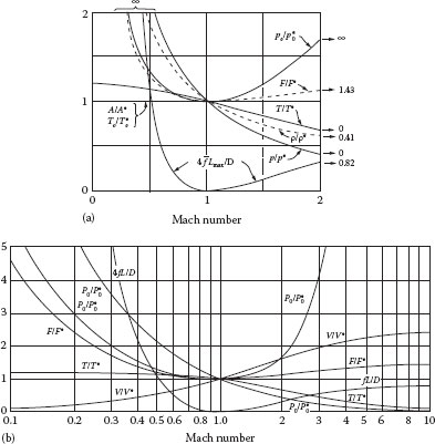
FIGURE 9.4 Fanno line functions for k = 1.4. (a) From Hall (1951) and (b) from Shapiro (1953).

For real gases, the “isentropic” exponents’ values change with temperature and pressure and differ from the ideal gas values. However, for fluids with k_Pρ higher than 1.2, the coefficient A_h ≈ 2 over a wide region of pressure and temperature, for all temperatures below the critical, except in the very vicinity of the critical point, as well as in the supercritical zone where the reduced pressure P_r = P/P_c does not exceed the reduced temperature T_r = T/T_c (P_r ≤ T_r). Then from Equations 9.96 and 9.98 it follows that it is possible to use the ideal gas equations (9.85 to 9.101) with an average value of k_Pρ instead of k.

In the case of gases with k_Pρ close to 1, the coefficient A ≈ 2 in the same region of reduced temperatures and pressures, and δ ≪ 1. Thus, for subsonic flow (N_Ma ≤ 1), we can set A = 2, δ = 0 in Equations 9.95 and 9.97, which gives

$\frac{4\overline{f}L}{D}{\overline{k}}_{P\text{ρ}}=\frac{1}{N_{Ma1}^2}-\frac{1}{N_{Ma2}^2}+2\ln \left(\frac{N_{Ma1}}{N_{Ma2}}\right)$

(9.108)

$\frac{P_2}{P_1}=\frac{N_{Ma1}}{N_{Ma2}}$

(9.109)

and

$\frac{P_2}{P_1}={\left\{1-\frac{G^2}{P_1{\text{ρ}}_1}\left[\frac{4fL}{D}-\frac{2}{{\overline{k}}_{P\text{ρ}}}\ln \left(\frac{P_2}{P_1}\right)\right]\right\}}^{1/2}$

(9.110)

Note that these equations differ from the isothermal equations (9.24) and (9.25) only by the one coefficient k_Pρ and the two coincide for k_Pρ = 1. Note also that the isentropic flow Equation (9.27) can be derived from Equations 9.84 and 9.85 by putting k_PT = 0.

While the isothermal flow model (Equation 9.24) approximates Fanno flow for small Mach numbers, the isentropic flow model Equation (9.27) is a good approximation when the flow approaches sonic. The “pseudo-isothermal” flow Equation (9.110) provides a good approximation for Fanno subsonic flow for the whole subsonic Mach number range (when 1 ≤ k_Pρ ≤ 1.2).

C.    SOLUTION OF HIGH-SPEED IDEAL GAS PROBLEMS

We will illustrate the procedure for solving the three types of pipe flow problems for high-speed ideal gas flows: unknown driving force, unknown flow rate, and unknown diameter.

1.  Unknown Driving Force

The unknown driving force can be either the upstream pressure, P₁, or the downstream pressure, P₂. However, one of these must be known, and the other is determined as follows.

Given: P₁, T₁, G, D, L, ε Find: P₂

1.  Calculate N_Re = DG/μ₁ and use this to find f₁ (Churchill Eq. or Moody diagram).

2.  Calculate N_Ma1 = (G/P₁)(RT₁/kM)^1/2. Use this with Equations 9.99, 9.101, and 9.102 or Figure 9.4 or Appendix I to find $\left(4f{L}_1^{*}/D_1\right),P_1/P*$ and T₁/T*. From these values and the given quantities, calculate $L_1^{*},P*$, and T*.

3.  Calculate $L_2^{*}=L_1^{*}-L$ and use this to calculate ${\left(4f_1{L}_2^{*}/D\right)}_2$. Use this with Figure 9.4 or Appendix I or Equations 9.99, 9.101, and 9.102 to determine N_Ma2, P₂/P*, and T₂/T*. (Note that Equation 9.99 is implicit in N_Ma2.) From these values, determine P₂ and T₂.

4.  Revise the value of the viscosity by evaluating it at an average temperature, (T₁ + T₂)/2, and pressure, (P₁ + P₂)/2. Use this to revise N_Re and hence f, and repeat steps 3 and 4 until the change is within acceptable limits.

2.  Unknown Flow Rate

The mass velocity (G) is the unknown in this case. This is equivalent to the mass flow rate because the pipe diameter is known. This requires a trial-and-error procedure because neither the Reynolds number nor the Mach numbers can be determined a priori.

Given: P₁, T₁, L, P₂, D, ε Find: G

1.  Assume a value for N_Ma1. Use Equations 9.101, 9.102, and 9.106 or Figure 9.4 or Appendix I to find P₁/P*, T₁/T*, and ${\left(4f{L}_1^{*}/D\right)}_1$. From these values and the given quantities, determine P* and T*.

2.  Calculate G₁ = N_Ma1P₁(kM/RT₁)^1/2 and N_Re1 = DG/μ. Using the latter, determine f₁ from the Churchill equation or Moody diagram.

3.  Calculate ${\left(4f{L}_2^{*}/D\right)}_2={\left(4f{L}_1^{*}/D\right)}_1-\left(4fL/D\right)$. Use this with Equation 9.99 (implicit) and Equations 9.102 and 9.103 or Figure 9.4 or Appendix I to find N_Ma2, P₂/P*, and T₂/T* at point 2.

4.  Calculate P₂ = (P₂/P*)P*, T₂ = (T₂/T*)T*, G₂ = N_Ma2P₂(kM/RT)^1/2, and N_Re = DG₂/μ. Use the latter to determine a revised value of f = f₂.

5.  Using f = (f₁ + f₂)/2 for the revised friction factor, repeat steps 3 and 4 until the change is within acceptable limits.

6.  Compare the given value of P₂ with the calculated value from step 4. If they agree, the answer is the calculated value of G₂ from step 4. If they do not agree, return to step 1 with a new guess for N_Ma1, and repeat the procedure until agreement is achieved.

3.  Unknown Diameter

The procedure for an unknown diameter involves a trial-and-error process similar to the one for the unknown flow rate.

Given: P₁, T₁, L, P₂, ṁ, ε Find: D

1.  Assume a value for N_Ma1 and use Equations 9.101, 9.102, and 9.106 or Figure 9.4 or Appendix I to find P₁/P*, T₁/T*, and ${\left(4f{L}_1^{*}/D\right)}_1$. Also, calculate G = N_Ma1P₁(kM/RT)^1/2, D = (4ṁ/πG)^1/2, and N_Re1 = DG/μ. Use N_Re1 and an assumed value of pipe wall roughness of 0.005 in. to find f₁ from the Churchill equation or Moody diagram.

2.  Calculate P₂/P* = (P₁/P*)(P₂/P*) and use this with Figure 9.4 or Appendix I or Equations 9.99, 9.101 (implicitly), and 9.102 to find N_Ma2, ${\left(4f{L}_2^{*}/D\right)}_2$ and T₂/T*. Calculate T₂ = (T₂/T*)(T*T₁)T₁ and use P₂ and T₂ to determine μ₂. Then use μ₂ to determine N_Re2 = DG/μ₂, which, with a wall roughness of 0.005 in., determines f₂ from the Churchill equation or Moody diagram.

3.  Using f = (f₁ + f₂)/2, calculate $L=L_1^{*}-L_2^{*}=\left[{\left(4f{L}_1^{*}/D\right)}_1-{\left(4f{L}_2^{*}/D\right)}_2\right]\left(D/4f\right)$.

4.  Compare the value of L calculated in step 3 with the given value, and the value of ε/D with that used in step 1. If they agree, the value of D determined in step 1 and the assumed value of ε are correct. If they do not agree, return to step 1, revise the assumed value of N_Ma1, and ε = 0.005 in., and repeat the entire procedure until agreement is achieved.

SUMMARY

The major points covered in this chapter include:

•  Understand and be able to apply the basic equations for ideal gas in pipes, for isothermal and adiabatic flow, including the determination of choked flow.

•  Know how to use the Expansion Factor approach for problems involving adiabatic flow in pipes.

•  Understand and be able to apply the generalized flow equations (under all flow conditions) to an ideal gas in pipes, for any Mach number.

•  Understand how to generalize the equations for ideal gases under any conditions, to any compressible fluid.

PROBLEMS

COMPRESSIBLE FLOW

1.  A 12 in. ID gas pipeline carries methane (molecular weight (M = 16) at a rate of 20,000 scfm. The gas enters the line at a pressure of 500 psia, and a compressor station is located every 100 miles to boost the pressure back up to 500 psia. The pipeline is isothermal at 70°F, and the compressors are adiabatic with an efficiency of 65%. What is the required horsepower for each compressor? Assume ideal gas behavior.

2.  Natural gas (CH₄) is transported through a 6 in. ID pipeline at a rate of 10,000 scfm. The compressor stations are 150 miles apart, and the compressor suction pressure is maintained at 10 psig above that at which choked flow would occur in the pipeline. The compressors are each two-stage, operate adiabatically with interstage cooling to 70°F, and have an efficiency of 60%. If the pipeline temperature is 70°F, calculate

(a)  The discharge pressure, interstage pressure, and compression ratio for the compressor stations

(b)  The horsepower required at each compressor station

3.  Natural gas (methane) is transported through a 20 in. sch 40 commercial steel pipeline at a rate of 30,000 scfm. The gas enters the line from a compressor at 100 psia and 70°F. Identical compressor stations are located every 10 miles along the line, and at each station the gas is recompressed to 100 psia and cooled to 70°F.

(a)  Determine the suction pressure at each compressor station.

(b)  Determine the horsepower required at each station if the compressors are 80% efficient.

(c)  How far apart could the compressor stations be located before the flow in the pipeline becomes choked?

4.  Natural gas (methane) is transported through an uninsulated 6 in. ID commercial steel pipeline, 1 mile long. The inlet pressure is 100 psia and the outlet pressure is 1 atm. What is the mass flow rate of the gas and the compressor power required to pump it? T₁ = 70°F, μ_gas = 0.02 cP.

5.  It is desired to transfer natural gas (CH₄) at a pressure of 200 psia and a flow rate of 1000 scfs through a 1 mile long uninsulated commercial steel pipeline into a storage tank at 20 psia. Can this be done using either a 6 or 12 in. ID pipe? What diameter pipe would you recommend? T₁ = 70°F, μ = 0.02 cP.

6.  A natural gas (methane) pipeline is designed to transport the gas at a rate of 5000 scfm. The pipe is 6 in. ID and the maximum pressure that the compressors can develop is 1500 psig. The compressor stations are located in the pipeline at the point at which the pressure drops to 100 psi above that at which choked flow would occur (i.e., the suction pressure for the compressor stations). If the design temperature for the pipeline is 60°F, the compressors are 60% efficient, and the compressor stations each operate with three stages and interstage cooling to 60°F, determine

(a)  The proper distance between compressor stations, in miles

(b)  The optimum interstage pressure and compression ratio for each compressor stage

(c)  The total horsepower required for each compressor station

7.  Ethylene gas leaves a compressor at a pressure of 3500 psig and is carried in a 2 in. sch 40 pipeline, 100 ft long, to a unit where the pressure is 500 psig. The line contains two plug valves, one swing check valve, and eight flanged elbows. If the temperature is 100°F, what is the flow rate (in scfm)?

8.  A 12 in. ID natural gas (methane) pipeline carries gas at a rate of 20,000 scfm. The compressor stations are 100 miles apart, and the discharge pressure of the compressors is 500 psia. If the temperature of the surroundings is 70°F, what is the required horsepower of each compressor station, assuming 65% efficiency? If the pipeline breaks 10 miles downstream of a compressor station, what will be the flow rate through the broken pipe?

9.  The pressure in a reactor fluctuates between 10 and 30 psig. It is necessary to feed air to the reactor at a constant rate of 20 lb_m/h from an air supply at 100 psig, 70°F. To do this, you insert an orifice into the air line that will provide the constant flow rate. What size (diameter) should the orifice be?

10.  Oxygen is fed to a reactor at a constant rate of 10 lb_m/s from a storage tank in which the pressure is constant at 100 psig and the temperature is 70°F. The pressure in the reactor fluctuates between 2 and 10 psig, so you want to insert a choke in the line to maintain the flow rate constant. If the choke is a 2 ft length of tubing, what should the ID of the tubing be?

11.  Methane is fed to a reactor at a rate of 10 lb_m/min. The methane is available in a pipeline at 20 psia, 70°F, but the pressure in the reactor fluctuates between 2 and 10 psia. To control the flow rate, you want to install an orifice plate that will choke the flow at the desired rate. What should the diameter of the orifice be?

12.  Ethylene gas (MW = 28, k = 1.3, μ = 0.1 cP) at 100°F is fed to a reaction vessel from a compressor through 100 ft of 2 in. sch 40 pipe containing 2 plug valves, one swing check valve, and 8 flanged elbows. If the compressor discharge pressure is 3500 psig and the pressure in the vessel is 500 psig, what is the flow rate of the gas, in scfm (1 atm, 60°F)?

13.  Nitrogen is fed from a high-pressure cylinder through ¼ ID stainless steel tubing, to an experimental unit. The line ruptures at a point that is 10 ft from the cylinder. If the pressure of the nitrogen in the cylinder is 3000 psig and the temperature is 70°F, what are the mass flow rate of the gas through the line and the pressure in the tubing at the point of the break?

14.  A storage tank contains ethylene at 200 psig and 70°F. If a 1 in. ID line that is 6 ft long containing a globe valve on the end is attached to the tank, what would the flow rate of gas be (in scfm) if

(a)  The valve is fully open?

(b)  The line breaks off right at the tank?

15.  A 2 in. sch 40 pipeline is connected to a storage tank containing ethylene at 100 psig and 80°C.

(a)  If the pipe breaks at a distance of 50 ft from the tank, determine the rate at which the ethylene will leak out of the pipe (in lb_m/s).

(b)  If the pipe breaks off right at the tank, what would the leak rate be?

16.  Saturated steam at 200 psig (388°F, specific volume, ν = 2.13 ft³/lb_m, μ = 0.015 cP) is fed from a header to a direct contact evaporator that operates at 10 psig. If the steam line is 2 in. sch 40 pipe, 50 ft long, and includes four flanged elbows and one globe valve, what is the steam flow rate in lb_m/h?

17.  Air is flowing from a tank at a pressure of 200 psia and 70°F through a venturi meter into another tank at a pressure of 50 psia. The venturi meter is mounted in a 6 ID pipe section (that is quite short) and has a throat diameter of 3 in. What is the mass flow rate of the air?

18.  A tank containing air at 100 psia and 70°F is punctured with a hole ¼ in. diameter. What is the mass flow rate of the air through the hole?

19.  A pressurized tank containing nitrogen at 800 psig is fitted with a globe valve, to which is attached a line with 10 ft of ¼ ID stainless steel tubing and three standard elbows. The temperature of the system is 70°F. If the valve is left wide open, what is the flow rate of nitrogen, in lb_m/s and also in scfm?

20.  Gaseous chlorine (M = 71) is transferred from a high-pressure storage tank at 500 psia and 60°F, through an insulated 2 in. sch 40 pipe 200 ft long, into another vessel where the pressure is 200 psia. What is the mass flow rate of the gas and its temperature at the point where it leaves the pipe?

21.  A storage tank contains ethylene at a pressure of 200 psig and a temperature of 70°F springs a leak. If the hole through which the gas is leaking is ½ in. diameter, what is the leakage rate of the ethylene, in scfm?

22.  A high-pressure cylinder containing N₂ at 200 psig and 70°F is connected by ¼ in. ID stainless steel tubing, 20 ft long, to a reactor in which the pressure is 15 psig. A pressure regulator at the upstream end of the tubing is used to control the pressure in the reactor, and hence the flow rate of the N₂ in the tubing.

(a)  If the regulator controls the pressure entering the tubing at 25 psig, what is the flow rate of N₂ (in scfm)?

(b)  If the regulator fails so that the full pressure from the cylinder is applied at the tubing entrance, what will be the flow rate of the N₂ into the reactor (in scfm)?

23.  Oxygen is supplied to an astronaut through an umbilical hose that is 7 m long. The pressure in the oxygen tank is 200 kPa at a temperature of 10°C, and the pressure in the space suit is 20 kPa. If the umbilical hose has an equivalent roughness of 0.01 mm, what should the hose diameter be to supply oxygen at a rate of 0.05 kg/s? If the suit springs a leak and the pressure drops to zero, at what rate will the oxygen escape?

24.  Ethylene (MW = 28) is transported from a storage tank, at 250 psig and 70°F, to a compressor station where the suction pressure is 100 psig. The transfer line is 1 in. sch 80, 500 ft long, and contains two ball valves and eight threaded elbows. An orifice meter with a diameter of 0.75 in. is installed near the entrance to the pipeline.

(a)  What is the flow rate of the ethylene through the pipeline, in scfh?

(b)  If the pipeline breaks at a point 200 ft from the storage tank and there are four elbows and one gate valve in the line between the tank and the break, what is the flow rate of the ethylene (in scfh)?

(c)  What is the differential pressure across the orifice for both cases (a) and (b), in inches of water?

25.  Air passes from a large reservoir at 70°F through an isentropic converging-diverging nozzle into the atmosphere. The area of the nozzle throat is 1 cm², and that of the exit is 2 cm². What is the reservoir pressure at which the flow in the nozzle just reaches sonic velocity, and what are the mass flow rate and exit Mach number under these conditions?

26.  Air is fed from a reservoir through a converging-diverging nozzle into a ½ in. ID drawn steel tube that is 15 ft long. The flow in the tube is adiabatic, and the reservoir temperature and pressure are 70°F and 200 psia.

(a)  What is the maximum flow rate (in lb_m/s) that can be achieved in the tube?

(b)  What is the maximum pressure at the tube exit at which this flow rate will be reached?

(c)  What is the temperature at this point under these conditions?

27.  A gas storage cylinder contains nitrogen at 250 psig and 70°F. Attached to the cylinder is a 3 in. long ¼ in. sch 40 stainless steel pipe nipple, and attached to that is a globe valve followed by a diaphragm valve. Attached to the diaphragm valve is a ¼ in. ID copper tubing line. Determine the mass flow rate of nitrogen (in lb_m/s), if

(a)  The copper tubing breaks off at a distance of 30 ft downstream of the diaphragm valve.

(b)  The pipe breaks off right at the cylinder.

28.  A compressor supplies natural gas (mainly CH₄) to a pipeline. The compressor suction pressure is 20 psig and the discharge pressure is 1000 psig. The pipe is 5 in. sch 40 and the ambient temperature is 80°F.

(a)  If the pipe breaks at a point 2 miles downstream from the compressor station, determine the rate at which the gas will escape (in scfm).

(b)  If the compressor efficiency is 80%, what power is required to drive it?

29.  You have to feed a gaseous reactant to a reactor at a constant rate of 1000 scfm. The gas is stored in a tank, at 80°F and 500 psig, that is located 20 ft from the reactor, in which the pressure fluctuates between 10 and 20 psig. You know that if the flow is choked in the feed line to the reactor, then the flow rate will be independent of the pressure in the reactor, which is what you desire. If the feed line has a roughness of 0.0018 in., what should its diameter be in order to satisfy your requirement? The gas has a MW of 35, an isentropic exponent of 1.35, and a viscosity of 0.01 cP at 80°F.

30.  A pressure vessel containing nitrogen at 300°F has a relief valve installed on top of the vessel. The valve is set to open at a set pressure of 125 psig and exhausts its contents at atmospheric pressure. The valve has a nozzle that has a smoothly rounded entrance and is 1.5 in. in diameter and 4 in. long, which limits the flow through the valve when it is open.

(a)  If the flow resistance in the piping between the tank and the valve, and from the valve to the atmospheric discharge, is neglected, determine the mass flow rate through the valve when it opens (in lb_m/s).

(b)  In reality, there is a 3 ft length of a 3 in. pipe between the tank and the valve, and a 6 ft length of a 4 in. pipe downstream of the valve discharge. What is the effect of including this piping on the calculated flow rate?

(Note: This problem can be solved more accurately using the methods given in Chapter 11)

31.  A storage tank contains ethylene at 80°F and has a relief valve that is set to open at a pressure of 250 psig. The valve must be sized to relieve the gas at a rate of 85 lb_m/s when it opens. The valve has a discharge coefficient (the ratio of the actual mass flux to the theoretical mass flux) of 0.975.

(Note: This problem can be solved more accurately using the methods given in Chapter 11).

(a)  What should be the diameter of the nozzle in the valve? What horsepower would be required to compress the gas from 1 atm to the maximum tank pressure at a rate equal to the flow rate through the valve, for

(b)  A single-stage compressor.

(c)  A two-stage compressor with intercooling. Assume a 100% efficiency for the compressor.

NOTATION

A	Cross-sectional area, [L2]
A,B,Ah,Bh	Coefficients in general compressible flow equations, [—]
c	Speed of sound, [L/t]
D	Diameter, [L]
ef	Energy dissipation per unit mass of fluid, [FL/M = L2/t2]
f	Fanning friction factor, [—]
F	Force, [F = ML/t2]
G	Mass flux, [M/tL2]
h	Enthalpy per unit mass, [FL/M = L2/t2]
k	Isentropic exponent ([= cp/cv] for ideal gas), [—]
K	Bulk modulus, [F/L2 = M/(Lt2)]
kPρ, kTP, kTρ	Isentropic exponents for real gas, [—]
Kf	Loss coefficient, [—]
L	Length, [L]
M	Molecular weight, [M/mol]
ṁ	Mass flow rate, [M/t]
NMa	Mach number, [—]
NRe	Reynolds number, [—]
P	Pressure, [F/L2 = M/(Lt2)]
q	Heat transferred to fluid per unit mass, [FL/M = L2/t2]
R	Gas constant, [FL/(t mol)]
T	Temperature, [T]
V	Spatial averaged velocity, [L/t]
w	Work done by fluid per unit mass, [FL/M = L2/t2]
Y	Expansion factor, [—]
Z	Compressibility factor, [—]
z	Vertical distance measured upward from reference plane, [L]

GREEK

$\widehat{\beta }$	Dimensionless thermal expansion coefficient, [—]
Γ	Fundamental derivative, [—]
γ	“Polytropic” exponent, [—]
$\widehat{\kappa }$	Dimensionless isothermal bulk modulus, [—]
ρ	Density, [M/L3]
μ	Viscosity, [Ft/L2 = M/Lt]
μJT	Joule–Thomson coefficient, [TL2/F = TLt2/M]

SUBSCRIPTS

1	Reference point 1
2	Reference point 2
c	Critical parameters (pressure, temperature)
r	Reduced parameters (pressure, temperature)
s	Constant entropy
T	Constant temperature

SUPERSCRIPTS

*	Sonic state

REFERENCES

Baltajiev, N., An investigation of real gas effects in supercritical CO₂ compressors. PhD Dissertation, MIT, Cambridge, MA, 2012.

Cheng, D., X. Fan, and M. Yang, Quasi-1D compressible flow of hydrocarbon fuel. Forty-Eighth AIAA/ASME/SAE/ASEE Joint Propulsion Conference & Exhibit, Atlanta, GA, 30 July–01 August, 2012.

Crane, C., Flow of fluids through valves, fittings and pipe, Technical Manual 410, Crane Co., New York, 1991 (and subsequent issues).

Hall, N.A., Thermodynamics of Fluid Flow, Prentice-Hall, Englewood Cliffs, NJ, 1951.

Holland, F.A. and R. Bragg, Fluid Flow for Chemical Engineers, 2nd edn., Edward Arnold, London, U.K., 1995.

Istomin, V.A., Real gas isentropic indexes and their use in thermodynamics of gases and gas dynamics, Russ. J. Phys. Chem. [c/c of Zhurnal Fizicheskoi Khimii], 72(3), 334–339, 1998.

Istomin, V.A., Real gas isentropic indices: Definition and basic relations, Russ. J. Phys. Chem. [c/c of Zhurnal Fizicheskoi Khimii], 71(6), 883–888, 1997.

Korelshteyn, L., Choked and near-choked real gas and two-phase flow analysis of discharge piping. Proceedings of 2015 AIChE Spring Meeting and 11th Global Congress of Process Safety, Austin, TX, 2015.

NIST (National Institute of Science and Technology), Standard Reference Database 23, Reference Fluid Thermodynamic and Transport Properties—REFPROP, Version 9.0 (and subsequent versions), 2010.

Oosthuizen, P.H. and W.E. Carscallen, Introduction to Compressible Fluid Flow, 2nd edn., CRC, Boca Raton, FL, 2013.

Saad, M.A., Compressible Fluid Flow, 2nd edn., Prentice Hall, Englewood Cliffs, NJ, 1992.

Shapiro, A.H., The Dynamics and Thermodynamics of Compressible Fluid Flow, Vol. I, Wiley, New York, 1953.

Thompson, P.A., A fundamental derivative in gas dynamics, Phys. Fluids, 14(9), 1843–1849, 1971.