
“Simple laws can very well describe complex structures. The miracle is not the complexity of our world, but the simplicity of the equations describing that complexity.”
—Sander Bais, b. 1945, Theoretical Physicist
In 1883, Osborne Reynolds conducted a classical experiment, illustrated in Figure 6.1, in which he measured the pressure drop, ΔP, as a function of flow rate, Q, for water in a tube. He found that, at low flow rates, the pressure drop was directly proportional to the flow rate, but as the flow rate was increased, a point was reached where the relation was no longer linear and the “noise” or scatter in the data increased considerably. At still higher flow rates, the data became more reproducible, but the relationship between the pressure drop and the flow rate became almost quadratic instead of linear.
To investigate this phenomenon further, Reynolds introduced a trace of dye into the flow to observe what was happening. At the low flow rates where the linear relationship (ΔP vs. Q) was observed, the dye was seen to remain a coherent, rather smooth thread throughout most of the tube except for a little dispersion due to molecular diffusion. However, where the data scatter occurred, the dye trace was seen to be rather unstable, and it broke up after a short distance. At still higher flow rates, where the quadratic relationship was observed, the dye dispersed almost immediately into a uniform “cloud” throughout the tube. The stable flow observed initially was called laminar because it was observed that the fluid elements moved in smooth layers or “lamella” relative to each other with no mixing. The unstable flow pattern, characterized by a high degree of mixing between the fluid elements, was called turbulent. Although the transition from laminar to turbulent flow occurs rather abruptly, there is nevertheless a transition region where the flow is unstable and not very reproducible.
Careful study of various fluids in tubes of different sizes has indicated that laminar flow in a tube persists up to a point where the value of the Reynolds number (NRe = DVρ/μ) is about 2000, and turbulent flow occurs when NRe is greater than about 4000, with a transition region in between. Actually, unstable flow (turbulence) occurs when disturbances to the flow are amplified, whereas laminar flow occurs when these disturbances are damped out by the viscous forces. Because turbulent flow cannot occur unless there are disturbances, studies have been conducted on systems in which extreme care has been taken to eliminate any disturbances due to irregularities in the boundary surfaces, sudden changes in direction, vibrations, etc. Under these conditions, it has been possible to sustain laminar flow in a tube to a Reynolds number of the order of 100,000 or more. However, under all but the most unusual conditions, there are sufficient natural disturbances in all practical systems that the laminar flow ceases and turbulence begins in a pipe at a Reynolds number of about 2000.
The physical significance of the Reynolds number can be appreciated better if it is rearranged as follows:
(6.1) |
The numerator (ρV2) is the flux of “inertial” momentum, carried by the fluid along the tube in the axial direction. The denominator (μV/D) is proportional to the viscous shear stress in the tube, which is equivalent to the “viscous” flux of momentum normal to the flow direction, that is, in the radial direction. Thus, the Reynolds number is the ratio of the inertial momentum flux in the flow direction to the viscous momentum flux in the transverse (radial) direction. Because viscous forces are a manifestation of intermolecular attractive forces, they are stabilizing, whereas inertial forces tend to pull the fluid elements apart and are therefore destabilizing. It is thus quite logical that stable (laminar) flow should occur at low Reynolds numbers where viscous forces dominate, whereas unstable (turbulent) flow occurs at high Reynolds numbers where inertial forces dominate. Also, laminar flows are dominated by viscosity and are independent of the fluid density, whereas fully turbulent flows are dominated by the fluid density and are independent of the fluid viscosity at high turbulence levels. For fluids flowing near solid boundaries (e.g., inside conduits or around solid bodies), viscous forces dominate in the immediate vicinity of the boundary, whereas for turbulent flows (high Reynolds numbers) inertial forces dominate in the region far from the boundary. We will consider both the laminar and turbulent flow of Newtonian and non-Newtonian fluids in pipes in this chapter.
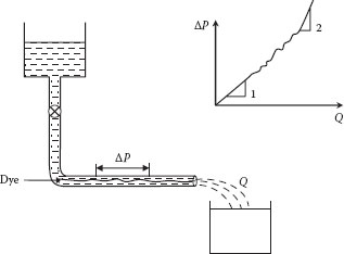
FIGURE 6.1 Reynolds’ experiment.
II. GENERAL RELATIONS FOR PIPE FLOWS
For steady, uniform, fully developed flow in a pipe (or any conduit), the conservation of mass, energy, and momentum equations can be arranged in specific forms that are most useful for the analysis of such problems. There are several different approaches to this analysis, as described in the following. Each of these is a general expression that is valid for both Newtonian and non-Newtonian fluids in either laminar or turbulent flow.
Consider a section of uniform cylindrical pipe of length L and radius R, inclined upward at an angle θ to the horizontal, as shown in Figure 6.2. The steady-state energy balance (or Bernoulli equation) applied to an incompressible fluid flowing in a uniform pipe can be written as
(6.2) |
where
Φ = P + ρgz
Kf = 4fL/D
f is the Fanning friction factor
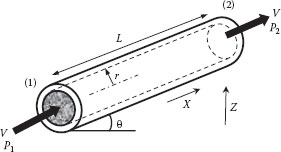
FIGURE 6.2 Steady flow in a uniform pipe.
Another approach is to write a momentum balance on a cylindrical volume of fluid of radius r and length L, centered on the pipe centerline (see Figure 6.2) as follows:
∑Fx = (P1 − P2)πr2 − πr2Lρg sin θ + 2πrLτrx = 0 |
(6.3) |
where τrx is the tangential shear stress in the x direction acting on the r surface of the fluid system. Solving Equation 6.3 for τrx gives
(6.4) |
where
ΔΦ = ΔP + ρgL sin θ = ΔP + ρgΔz
τw is the stress exerted by the fluid on the tube wall (i.e., τw = (−τrx)r=R)
Note that this can also be obtained directly by integrating the axial component of the microscopic momentum equation of motion in cylindrical coordinates (i.e., the z-component equation in Appendix E).
Equation 6.4 is equivalent to Equation 6.2, because
f = τwρ V2/2 = Kf4L/D = ef(4L/D)(V2/2) |
(6.5) |
Note that from Equation 6.4 the shear stress is negative, that is, the fluid outside the cylindrical system of radius r is moving slower than the fluid inside the system and hence exerts a force in the −x direction on the fluid in the system, which is bounded by the r surface. However, the stress at the wall (τw) is defined as the force exerted in the +x direction by the fluid on the wall (which is positive). The fact that the energy balance equation (Bernoulli) and the momentum balance both give identical results for this particular problem is not a general result. In general, the momentum balance is a vector equation, but when applied to this 1-D problem the result is identical to the (scalar) Bernoulli equation. The momentum balance is most useful in determining forces on fluid systems involving multidirectional flows, such as flows through pipe bends and elbows. This is illustrated later on.
Continuity provides another relationship between the volumetric flow rate (Q) passing through a given cross section in the pipe and the local velocity (vx), that is,
Q = ∫Avx dA = π R∫o2rvx dr = π∫Avxdr2 |
(6.6) |
This can be integrated by parts, as follows:
Q = π∫Avx dr2 = −π∫Ar2 dvx =−π R∫0r2 dvxdr dr |
(6.7) |
Thus, if the radial dependence of the velocity or shear rate (dvx/dr) is known or can be found, the flow rate can be determined directly from Equation 6.7. Application of this principle to laminar flow is shown in the following section.
A different, but related, approach to pipe flow that provides additional insight involves consideration of the rate at which energy is dissipated per unit volume of fluid. In general, the rate of energy (or power) expended in a system subjected to a force →F
˙ef = ef˙m = efρQ = ∫Vol↔τ : ∇→v d ˜V |
(6.8) |
where
↔τ
˜V
The “:” operator in Equation (6.8) represents the scalar product of two dyads. Thus, integration of the local rate of energy dissipation throughout the entire flow volume, along with the Bernoulli equation, which relates the energy dissipated per unit mass (ef) to the driving force (ΔΦ), can be used to determine the flow rate. All of the equations to this point are general because they apply to any fluid (Newtonian or non-Newtonian) in any type of flow (laminar or turbulent) in steady, fully developed flow in a uniform cylindrical tube at any orientation. The following section will illustrate the application of these relations to laminar flow in a pipe.
For a Newtonian fluid in laminar flow
(6.9) |
When the velocity gradient from Equation 6.9 is substituted into Equation 6.7 and Equation 6.4 is used to eliminate the shear stress, Equation 6.7 becomes
Q = −π R∫0r2 dvxdr dr = −πμ R∫0r2τrx dr = πτwμR R∫0r3 dr |
(6.10) |
or
Q = πτwR34μ = − π∇ΦR48μL = − π∇ΦD4128μL |
(6.11) |
Equation 6.11 is known as the Hagen–Poiseuille equation for laminar flow of a Newtonian fluid in a tube.
This result can also be derived by equating the shear stress for a Newtonian fluid (Equation 6.9) to the expression obtained from the momentum balance for tube flow (Equation 6.4) and integrating (using the no-slip condition at the tube wall) to obtain the velocity profile:
(6.12) |
Inserting this into Equation 6.6 and integrating over the tube cross section gives Equation 6.11 for the volumetric flow rate.
Another approach is to use the Bernoulli equation (Equation 6.2) and Equation 6.8 for the friction loss term ef. The integral in the latter equation is evaluated in a manner similar to that leading to Equation 6.10, as follows. Eliminating ef between Equation 6.8 and the Bernoulli equation (Equation 6.2, i.e., ρef = −∇Φ) leads directly to
which is, again, the Hagen–Poiseuille Equation (Equation 6.11).
If the wall stress (τw) in Equation 6.11 is expressed in terms of the Fanning friction factor (i.e., τw = fρV2/2) and the result solved for f, the dimensionless form of the Hagen–Poiseuille equation follows:
(6.14) |
It may be recalled that application of dimensional analysis (Chapter 2) showed that the steady fully developed laminar flow of a Newtonian fluid in a cylindrical tube can be characterized by a single dimensionless group, which is seen from Equation 6.14 to be the product fNRe (note that this group is independent of the fluid density, which cancels out). Since there is only one dimensionless group, it follows that this group must be the same (i.e., constant) for all such flows, regardless of the fluid viscosity or density, the size of the tube, the flow rate, etc. Although the magnitude of this constant could not be obtained from dimensional analysis, we have shown from basic principles that this value is 16, which is also in agreement with experimental observations. Equation 6.14 is valid for a Newtonian fluid with NRe < 2000, as previously discussed.
It should be emphasized here that these results are applicable only to “fully developed” flow (i.e., far enough from the tube entrance so that the flow conditions are independent of the distance downstream). However, if the fluid enters a pipe with a uniform (“plug”) velocity distribution, a minimum hydrodynamic entry length (Le) is required for the parabolic velocity flow profile (Equation 6.12) to develop and the pressure gradient to become uniform. It can be shown that this (dimensionless) “hydrodynamic entry length” is approximately Le/D = NRe/20.
As previously noted, if the Reynolds number in the tube is larger than about 2000, the flow will no longer be laminar. Because fluid elements in contact with a stationary solid boundary are also stationary (i.e., the fluid sticks to the wall), the velocity increases from zero at the boundary to a maximum value at some distance from the boundary. For uniform flow in a symmetrical duct, the maximum velocity occurs at the centerline of the duct. The region of flow over which the velocity varies with the distance from the boundary is called the boundary layer and is illustrated in Figure 6.3.
Because the fluid velocity at a solid boundary is zero, there will always be a region adjacent to the wall that is laminar. This is called the laminar sublayer and is designated δL in Figure 6.3 (in which the distances are not to scale, as the laminar sublayer is normally quite small). Note that for tube flow, if NRe < 2000 the entire flow is laminar and δL = R. The turbulent boundary layer (δT) includes the region in the vicinity of the wall in which the flow is turbulent and the velocity varies with the distance from the wall (y). Beyond this region, the fluid is almost completely mixed in what is often called the turbulent core, in which the velocity is independent of y. The transition from the laminar sublayer to the turbulent boundary layer is gradual, not abrupt, and the transition region is called the buffer zone.
The velocity field in turbulent flow can be described by a local “mean” (or time-average) velocity, upon which is superimposed a time-dependent fluctuating component or “eddy.” Even in “1-D” flow, in which the overall average velocity has only one directional component, that is, the turbulent core (as illustrated in Figure 6.3), the turbulent eddies have a 3D structure. Thus, for the flow illustrated in Figure 6.3, the local velocity components are
vx (y, t) = ˉvx(y) + v′x(y, t)vy (y, t) = 0 + v′y(y, t)vz (y, t) = 0 + v′z(y, t) |
(6.15) |
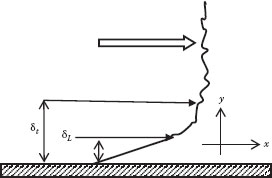
FIGURE 6.3 The boundary layer (not to scale).
The time-average velocity (ˉvx)
ˉvx = 1T T∫0vx dt so that T∫0v′x dt = 0 |
(6.16) |
Now the eddies transport momentum and the corresponding momentum flux components are equivalent to (negative) fluctuating stress components, as follows:
These “turbulent momentum flux components” are also called Reynolds stresses. Thus, the total stress in a Newtonian fluid in turbulent flow is composed of both viscous and turbulent (Reynolds) stresses:
τij = μ (∂ˉvi∂xj + ∂ˉvj∂xi) − ρv′iv′j |
(6.18) |
Although Equation 6.18 can be used to eliminate the stress components from the general microscopic equations of motion, a solution for the turbulent flow field still cannot be obtained unless some information about the spatial dependence and structure of the eddy velocities or turbulent (Reynolds) stresses is known. A classical (simplified) model for the turbulent stresses, attributed to Prandtl, is outlined in the following section.
Turbulent eddies (with fluctuating velocity components v′xv′y, v′z
(6.19) |
He also assumed that each eddy moves a distance l (the “mixing length”) during the time it takes to exchange its momentum with the mean flow, that is, the eddy “lifetime”
(6.20) |
Using Equation 6.20 to eliminate the eddy velocity from Equation 6.19 gives
(6.21) |
where
(6.22) |
is called the eddy viscosity. Note that the eddy viscosity is not a fluid property; it is a function of the eddy characteristics (e.g., the mixing length or the degree of turbulence) and the mean velocity gradient. The only fluid property involved is the density because turbulent momentum transport is an inertial (i.e., mass dominated) effect. Since turbulence (and all motion) is zero at the wall, Prandtl further assumed that the mixing length should be proportional to the distance from the wall, that is,
(6.23) |
Because these relations apply only in the vicinity of the wall, Prandtl also assumed that the eddy (Reynolds) stress must be of the same order as the wall stress, that is,
(6.24) |
Integrating Equation 6.24 over the turbulent boundary layer (from y1, the edge of the buffer layer, to y) gives
(6.25) |
This equation is called the von Karman equation (or, sometimes, the “law of the wall”) and can be written in the following dimensionless form:
(6.26) |
where
v+ = ˉvxv∗ = ˉvxV √2f, y+ = yv*ρμ = yVρμ √f2 |
(6.27) |
The term
(6.28) |
is called the friction velocity because it is a wall stress parameter with dimensions of velocity. The parameters κ and A in the von Karman equation have been determined from experimental data on Newtonian fluids in smooth pipes to be κ = 0.4 and A = 5.5. Equation 6.26 applies only within the turbulent boundary layer (outside the buffer region), which has been found empirically to correspond to y+ ≥ 26. Within the laminar sublayer, the turbulent eddies are negligible, so that
(6.29) |
The corresponding dimensionless form of this equation is
(6.30) |
or
(6.31) |
Equation 6.31 applies to the laminar sublayer region in a Newtonian fluid, which has been found to correspond to 0 ≤ y+ ≤ 5. The intermediate region or “buffer zone” between the laminar sublayer and the turbulent boundary layer can be represented by the empirical equation
(6.32) |
which applies for 5 < y+ < 26.
4. Friction Loss in Smooth Pipe
For a Newtonian fluid in a smooth pipe, these equations can be integrated over the pipe cross section to give the average fluid velocity, for example,
V = 2R2 R∫0ˉvxr dr = 2v∗ 1∫0v+ (1−x)dx |
(6.33) |
where x = y/R = 1 − r/R is the dimensionless distance from the wall. If the von Karman equation (Equation 6.26) for v+ is introduced into this equation and the laminar sublayer and buffer zones are neglected, the integral can be evaluated and the result solved for 1/√f to give
(6.34) |
The constants in this equation were modified by Nikuradse from observed data taken in smooth pipe as follows:
(6.35) |
This is also known as the von Karman–Nikuradse equation and agrees well with observations for friction loss in smooth pipe over the range 5 × 10³ < NRe < 5 × 10⁶.
An alternative equation for smooth tubes was derived by Blasius based on observations that the mean velocity profile in the tube could be represented approximately by
(6.36) |
A corresponding expression for the friction factor can be obtained by writing this expression in dimensionless form and substituting the result into Equation 6.33. Evaluating the integral and solving for f gives the Blasius equation
(6.37) |
This represents the friction factor for Newtonian fluids in smooth tubes quite well over a range of Reynolds numbers from about 5000 to 105. The Prandtl mixing length theory and the von Karman and Blasius equations are referred to as “semiempirical” models. That is, even though these models result from a process of logical reasoning, the results cannot be deduced solely from first principles because they require the introduction of certain parameters that can be evaluated only experimentally.
5. Friction Loss in Rough Tubes
All models for turbulent flows are semiempirical in nature, so it is necessary to rely upon empirical observations (e.g., data) for a quantitative description of friction loss in such flows. For Newtonian fluids in long tubes, we have shown from dimensional analysis that the friction factor should be a unique function of the Reynolds number and the relative roughness of the tube wall. This result has been used to correlate a wide range of measurements in tubes of a variety of sizes and roughness factors, with a variety of fluids and for wide range of flow rates in terms of a generalized plot of f versus NRe, with ε/D as a parameter. This correlation, shown in Figure 6.4, is called a Moody diagram.
The laminar region (for NRe < 2000) is represented by the theoretical Hagen–Poiseuille equation (Equation 6.14), which is plotted in Figure 6.4 as the f = 16/NRe line. In this region, the only fluid property that influences the friction loss (or energy dissipation) is the viscosity, as the density cancels out. Furthermore, the roughness has a negligible effect in laminar flow, as will be explained shortly. The “critical zone” is the range of transition from laminar to turbulent flow, which corresponds to values of NRe from about 2000 to 4000. Data are not very reproducible in this region, where the friction factor depends strongly on both the Reynolds number and relative roughness. The region in the upper right of the diagram, where the relative roughness lines are horizontal, is called “complete turbulence,” or “fully turbulent.” In this region, the friction factor is independent of Reynolds number (i.e., independent of viscosity) and is a function only of the relative roughness. For turbulence in smooth tubes, the semiempirical Prandtl–von Karman/Nikuradse or Blasius models represent the friction factor quite well.
Whether a tube is hydraulically “smooth” or “rough” depends upon the size of the wall roughness elements relative to the thickness of the laminar sublayer. Because laminar flow is stable, if the flow perturbations due to the roughness elements lie entirely within the laminar wall region, the disturbances will be damped out and will not affect the rest of the flow field. However, if the roughness elements protrude through the laminar sublayer into the turbulent region, which is unstable, the disturbance will grow, thus enhancing the Reynolds stresses and consequently the energy dissipation or friction loss in the pipe. Because the thickness of the laminar sublayer decreases as the Reynolds number increases, a tube with a given roughness may be hydraulically smooth at a low Reynolds number but it may become hydraulically rough at a high Reynolds number.
6. Friction Loss in Rough Pipe
For rough tubes in turbulent flow (NRe > 4000), the von Karman equation was modified empirically by Colebrook to include the effect of wall roughness, as follows:
1√f = −4 log [ε/D3.7 + 1.255NRe√f] |
(6.38) |
The term NRe√f
(6.39) |
and is independent of velocity or flow rate. Thus, the dimensionless groups in the Colebrook equation are in a form that is convenient if the flow rate is to be found and the allowable friction loss (e.g., driving force), tube size, and fluid properties are known.
In the fully turbulent region, f is independent of NRe, so that the Colebrook equation reduces to
(6.40) |
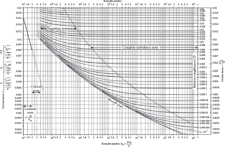
FIGURE 6.4 Moody diagram.
Just as for laminar flow, a minimum hydrodynamic entry length (Le) is required for the flow profile to become fully developed in turbulent flow. This length depends on the exact nature of the flow conditions at the tube entrance, but has been shown to be on the order of Le/D = 0.623N0.25Re
The actual size of the roughness elements on the conduit wall obviously varies with the method of manufacturing as well as from one material to another, with age and usage, and with the amount of dirt, scale, etc. Characteristic values of wall roughness have been determined for various materials, as shown in Table 6.1. The most common pipe material—clean, new commercial steel or wrought iron—has been found to have an effective roughness of about 0.0018 in. (0.045 mm). For other surfaces, such as concrete and wood, it may vary by as much as several orders of magnitude, depending upon the nature of the surface finish. Conduit surfaces artificially roughened by sand grains of various sizes were studied initially by Nikuradse, and measurements of f and NRe were plotted to establish the reference curves for various known values of ε/D for these surfaces, as shown on the Moody diagram. The equivalent roughness factors for other materials are determined from similar measurements in conduits made of the material, by plotting the data on the Moody diagram and comparing the results with the reference curves (or by using the Colebrook equation). For this reason, these roughness values are sometimes termed the equivalent sand grain roughness.
Equivalent Roughness of Various Surfaces
Material |
Condition |
Roughness Range |
Recommended |
Drawn brass, copper, stainless |
New |
0.01−0.0015 mm |
0.002 mm |
(0.0004−0.00006 in.) |
(0.00008 in.) |
||
Commercial steel |
New |
0.1−0.02 mm |
0.045 mm |
(0.004−0.0008 in.) |
(0.0018 in.) |
||
Light rust |
1.0−0.15 mm |
0.3 mm |
|
(0.04−0.006 in.) |
(0.015 in.) |
||
General rust |
3.0−1.0 mm |
2.0 mm |
|
(0.1−0.04 in.) |
(0.08 in.) |
||
Iron |
Wrought, new |
0.045 mm |
0.045 mm |
(0.002 in.) |
(0.002 in.) |
||
Cast, new |
1.0−0.25 mm |
0.30 mm |
|
(0.04−0.01 in.) |
(0.025 in.) |
||
Galvanized |
0.15−0.025 mm |
0.15 mm |
|
(0.006−0.001 in.) |
(0.006 in.) |
||
Asphalt coated |
1.0−0.1 mm |
0.15 mm |
|
(0.04−0.004 in.) |
(0.006 in.) |
||
Sheet metal |
Ducts |
0.1−0.02 mm |
0.03 mm |
Smooth joints |
(0.004−0.0008 in.) |
(0.0012 in.) |
|
Concrete |
Very smooth |
0.18−0.025 mm |
0.04 mm |
(0.007−0.001 in.) |
(0.0016 in.) |
||
Wood floated, brushed |
0.8−0.2 mm |
0.3 mm |
|
(0.03−0.007 in.) |
(0.012 in.) |
||
Rough, visible form marks |
2.5−0.8 mm |
2.0 mm |
|
(0.1−0.03 in.) |
(0.08 in.) |
||
Wood |
Stave, used |
1.0−0.25 mm |
0.5 mm |
(0.035−0.01 in.) |
(0.02 in.) |
||
Glass or plastic |
Drawn tubing |
0.01−0.0015 mm |
0.002 mm |
(0.0004−0.00006 in.) |
(0.00008 in.) |
||
Rubber |
Smooth tubing |
0.07−0.006 mm |
0.01 mm |
(0.003−0.00025 in.) |
(0.0004 in.) |
||
Wire reinforced |
4.0−0.3 mm |
1.0 mm |
|
(0.15−0.01 in.) |
(0.04 in.) |
The expressions for the friction factor in both laminar and turbulent flow were combined into a single expression by Churchill (1977) as follows:
f = 2[(8NRe)12 + 1(A+B)3/2]1/12 |
(6.41) |
where
A = [2.457 ln (1(7/NRe)0.9 + (0.27 ε/D))]16
and
B = (37,530NRe)16
Equation 6.41 adequately represents the Fanning friction factor over the entire range of Reynolds numbers, from laminar to fully turbulent, within the accuracy of the data used to construct the Moody diagram. It also gives a reasonable estimate for the intermediate or transition region between laminar and turbulent flow. Note that it is explicit in f.
Corresponding expressions for the friction loss in laminar and turbulent flow for non-Newtonian fluids in pipes for the two simplest (two-parameter) models—the power law and Bingham plastic—can be evaluated in a similar manner. The power law model is very popular for representing the viscosity of a wide variety of non-Newtonian fluids because of its simplicity and versatility. However, extreme care should be exercised in its application. Because the model breaks down at both very low and very high shear rates, any application involving extrapolation beyond the range of shear stress (or shear rate) represented by the data used to determine the model parameters can lead to misleading or erroneous results. Both laminar and turbulent pipe flow of highly loaded slurries of fine particles, for example, can often be adequately represented by either of these two models over an appreciable shear rate range, as shown by Darby et al. (1992).
Because the shear stress and shear rate are negative in pipe flow, the appropriate form of the power law model for laminar pipe flow is
(6.42) |
By equating the shear stress from Equations 6.42 and 6.4, solving for the velocity gradient, and introducing the result into Equation 6.7 (as was done for the Newtonian fluid), the flow rate is found to be
Q = π(τwmR)1/n R∫0r2+1/n dr = π(τwmR)1/n (n3n+1)R(3n+1)/n |
(6.43) |
This is the power law equivalent of the Newtonian Hagen–Poiseuille equation, which it reduces to if n = 1. It can be written in dimensionless form by expressing the wall stress in terms of the friction factor using Equation 6.5, solving for f, and equating the result to 16/NRe (i.e., the form of the Newtonian result). The result is an expression that is identical to the dimensionless Hagen–Poiseuille equation
(6.44) |
which defines the Reynolds number for a power law fluid as
NRe, pl = 8DnV2−nρm[2(3n + 1)/n]n |
(6.45) |
It should be noted that a dimensional analysis of this problem results in one more dimensionless group than for the Newtonian fluid because there is one more fluid rheological property (e.g., m and n for the power law fluid vs. μ for the Newtonian fluid). However, the parameter n is itself dimensionless and thus constitutes the additional “dimensionless group,” even though it is integrated into the Reynolds number as it has been defined here. Note also that because n is an empirical parameter and can take on any value, the units in expressions for power law fluids can be complex. Thus, the calculations are simplified if a scientific system of dimensions/units is used (e.g., SI or cgs), which avoids the necessity of introducing the conversion factor gc. In fact, the evaluation of most dimensionless groups is usually simplified by the use of scientific units.
Dodge and Metzner (1959) modified the von Karman equation to apply to power law fluids, with the following result:
1√f = 4n0.75 log [NRe, pl f(1−n)/2] − 0.4n1.2 |
(6.46) |
Like the von Karman equation, this equation is implicit in f. Equation 6.46 can be applied to any non-Newtonian fluid if the parameter n is interpreted to be the point slope of the shear stress versus shear rate plot from (laminar) viscosity measurements, at the wall shear stress (or shear rate) corresponding to the conditions of interest in turbulent flow. However, it is not a simple matter to acquire the needed data over the appropriate range, or to solve the equation for f for a given flow rate and pipe diameter, in turbulent flow.
Note that there is no effect of pipe wall roughness in Equation 6.46, in contrast to the case for Newtonian fluids. There are insufficient data in the literature to provide a reliable estimate of the effect of roughness on friction loss for non-Newtonian fluids in turbulent flow. However, the evidence that does exist suggests that the roughness is not as significant for non-Newtonian fluids as for Newtonian fluids. This is partly due to the fact that the majority of non-Newtonian turbulent flows lie in the low Reynolds number range and partly due to the fact that the laminar boundary layer tends to be thicker for non-Newtonian fluids than for Newtonian fluids (i.e., the flows are generally in the “hydraulically smooth” range for common pipe materials).
An expression that represents the friction factor for the power law fluid over the entire range of Reynolds numbers (laminar through turbulent) and encompasses Equations 6.44 and 6.46 has been given by Darby et al. (1992):
f = (1−α)fL + α[f−8T + f−8Tr]1/8 |
(6.47) |
where
(6.48) |
fTr = 1.79 × 10⁻⁴ exp [−5.24 n]N0.414+0.757nRe, pl |
(6.49) |
fT = 0.0682n−1/2(NRe, pl)1/(1.87 + 2.39 n) |
(6.50) |
The parameter α is given by
(6.51) |
where
(6.52) |
and NRe,plc is the critical power law Reynolds number at which laminar flow ceases
(6.53) |
Equation 6.48 applies for NRe, pl < NRe, plc, Equation 6.49 applies for NRe, plc < NRe, pl < 4000, Equation 6.50 applies for 4000 < NRe, pl < 105, and all are encompassed by Equation 6.47 for all values of NRe,pl.
The Bingham plastic model usually provides a good representation for the viscosity of concentrated slurries, suspensions, emulsions, foams, etc. Such materials often exhibit a yield stress that must be exceeded before the material will flow at a significant rate. Other examples include paint, shaving cream, and mayonnaise. There are also many fluids, such as blood, that may have a yield stress that is not as pronounced.
It is recalled that a “plastic” is really two materials. At low stresses below the critical or yield stress (τo), the material behaves as a solid, whereas for stresses above the yield stress, the material behaves as a fluid. The Bingham model for this behavior is
For |τ| < τo : ˙γ = 0For |τ| > τo: τ = ± τo + μ∞˙γ |
(6.54) |
Because the shear stress and shear rate can be either positive or negative, the plus/minus sign in Equation 6.54 is “plus” in the former case, and “minus” in the latter. For pipe flow, since the shear stress and shear rate are both negative, the appropriate form of the model is
For |τrx| < τo : dvxdr = 0For |τrx| > τo: τrx = − τo + μ∞ dvxdr |
(6.55) |
Because the shear stress is always zero at the centerline in pipe flow and increases linearly with distance from the center toward the wall (Equation 6.4), there will be a finite distance from the center over which the stress is always less than the yield stress. In this region, the material has solid-like properties and does not yield but moves as a rigid plug. The radius of this plug (ro) is, from Equation 6.4:
(6.56) |
Because the stress outside this plug region exceeds the yield stress, the material will deform or flow as a fluid between the plug and the wall. The flow rate must thus be determined by combining the flow rate of the “plug” with that of the “fluid” region:
Q = ∫Avx dA = Qplug + π R2∫r2ovx dr2 |
(6.57) |
Evaluating the integral by parts and noting that the Qplug term cancels with πr2oVplug
(6.58) |
When Equation 6.55 is used for the shear rate (˙γ = dvx/dr)
Q = π R3 τw4μ∞ [1− 43 (τoτw) + 13(τoτw)4] |
(6.59) |
This equation is known as the Buckingham–Reiner equation. It can be cast in dimensionless form and rearranged as follows:
fL = 16NRe [1 + 16 NHeNRe − 13 N4Hef3LN7Re] ≈ 16NRe [1 + NHe8 NRe] |
(6.60) |
where the Reynolds number is given by
(6.61) |
and
(6.62) |
is the Hedstrom number. Although the dimensionless Buckingham–Reiner equation is implicit in f, the approximate expression on the far right of Equation 6.60 follows from considerations of Equation 7.41 (Chapter 7) and is an excellent explicit approximation for the laminar friction factor. Note that the Bingham plastic model reduces to a Newtonian fluid if τo = 0 =NHe. In this case, Equation 6.60 reduces to the Newtonian result, that is, f = 16/NRe (see Equation 6.14). Note that there are actually only two independent dimensionless groups in Equation 6.60 (consistent with the results of dimensional analysis for a fluid with two rheological properties, τo and μ∞), which are the combined groups fNRe and NHe/NRe. The ratio NHe/NRe is also called the Bingham number, NBi = Dτo/μ∞V. The Buckingham–Reiner equation is implicit in f, so it must be solved by iteration for known values of NRe and NHe. However, the approximate expression on the right of Equation 6.60 is explicit in f and gives an excellent approximation for f in almost all cases.
For the Bingham plastic, there is no abrupt transition from laminar to turbulent flow as is observed for Newtonian fluids. Instead, there is a gradual deviation from purely laminar flow to fully turbulent flow. For turbulent flow, the friction factor can be represented by the empirical expression of Darby and Melson (1981) (as modified by Darby et al. (1992))
(6.63) |
where
a = −1.47 [ 1+ 0.146exp (−2.9 × 10⁻⁵ NHe)] |
(6.64) |
The friction factor for a Bingham plastic can be calculated for any Reynolds number, from laminar through turbulent, from the equation
(6.65) |
where
(6.66) |
In Equation 6.65, fT is given by Equation 6.63 and fL is given by Equation 6.60.
There are three typical problems encountered in pipe flows, depending upon what is known and what is to be found. These are the “unknown driving force,” “unknown flow rate,” and “unknown diameter” problems. We will outline here the procedure for the solution of each of these for both Newtonian and non-Newtonian (power law and Bingham plastic) fluids. A fourth problem, perhaps of even more practical interest for piping system design, is the “most economical diameter” problem that will be considered in Chapter 7.
We note first that the Bernoulli equation can be written in terms of the driving force DF as
(6.67) |
where
ef = (4 fLD) (v22) = 32 fLQ2π2D5 |
(6.68) |
and
(6.69) |
DF represents the net energy input into the fluid per unit mass (or the net “driving force”) and is the combination of static head, pressure difference, and pump work. When any of the terms in Equation 6.69 are negative, they represent a positive “driving force” (or energy input) for moving the fluid through the pipe. Positive terms represent forces resisting the flow, for example, an increase in elevation, pressure, etc., correspond to a negative driving force.
We will use the Bernoulli equation in the form of Equation 6.67 for analyzing pipe flows and we will use the total volumetric flow rate (Q) as the flow variable instead of the velocity, because this is the usual measure of capacity in a pipeline. For Newtonian fluids, the problem thus reduces to a relation between the three dimensionless variables:
NRe = 4QρπDμ, f = efπ2D532LQ2, εD |
(6.70) |
For a uniform pipe, the velocity is everywhere the same so the kinetic energy terms cancel out. In many other applications, the kinetic energy terms are often negligible or cancel out as well, although this should be verified for each situation.
For this problem, we want to know the net driving force (DF) that is required to move a given fluid (μ, ρ) at a specified rate (Q) through a specified pipe (D, L, ε). The Bernoulli equation in the form DF = ef applies.
The “knowns” and “unknowns” in this case are as follows:
Given: Q, μ, ρ, D, L, ε Find: DF
All the relevant variables and parameters are uniquely related through the three dimensionless variables f, NRe, and ε/D by the Moody diagram or the Churchill equation. Furthermore, the unknown (DF = ef) appears in only one of these groups (f). The procedure is thus straightforward:
1. Calculate the Reynolds number from Equation 6.70.
2. Calculate ε/D.
3. Determine f from the Moody diagram or Churchill equation (Equation 6.41) (if NRe < 2000, use f = 16/NRe).
4. Calculate ef (hence DF) from the Bernoulli equation, Equation 6.67.
From the resulting value of DF, the required pump head (−w/g), can be determined, for example, from a knowledge of the upstream and downstream pressures and elevations using Equation 6.69.
The equivalent problem statement is as follows:
Given: Q, m, n, ρ, D, L Find: DF
Note that we have an additional fluid property (m and n instead of μ), but we also assume that pipe roughness has a negligible effect, so that the total number of variables is the same. The corresponding dimensionless variables are f, NRe,pl, and n (which are related by Equation 6.47), and the unknown (DF = ef) appears in only one group (f). The procedure just followed for the Newtonian fluid can thus also be applied to a power law fluid if the appropriate equations are used, as follows:
1. Calculate the Reynolds number (NRe, pl) using Equation 6.45 and the volumetric flow rate instead of the velocity, that is,
NRe, pl = 27−3n ρQ2−nmπ2−n D4−3n (n3n+1)n |
(6.71) |
2. Calculate f from Equation 6.47.
3. Calculate ef (hence DF) from Equation 6.68.
The problem statement is as follows:
Given: Q, μ∞, τo, ρ, D, and L Find: DF
The number of variables is the same as in the foregoing problems; hence, the number of groups relating these variables is the same. For the Bingham plastic, these are f, NRe, and NHe, which are related by Equation 6.65 (along with Equations 6.60 and 6.63). The unknown (DF = ef) appears only in f, as before. The solution procedure is similar to that followed for Newtonian and power law fluids.
1. Calculate the Reynolds number:
(6.72) |
2. Calculate the Hedstrom number:
(6.73) |
3. Determine f from Equations 6.65, 6.63, and 6.60.
4. Calculate ef, hence DF, from Equation 6.68.
Example 6.1 Slurry Draining from Tank
Find the static head required to provide a flow of 150 gpm (gallons/min) for a Bingham plastic slurry through a 3 in. ID pipe, 400 ft long (See Figure E6.1). The slurry properties are as follows: density 1.8 g/cm3, yield stress 150 dyn/cm2, and limiting viscosity of 85 cP.
Solution:
As fluid properties are often expressed in cgs units, it is convenient to use these units for all variables in the problem. Therefore, we obtain the following:
Q = (150 gpm)(63.1 cm3/s and 1/gpm) = 9470 cm3/sD = 3 in. = 7.62 cmL = 400 ft = 12,300 cmτo = 150 dyn/cm2 = 150 g/(cm s2)μ∞ = 85 cP = 0.85 P = 0.85 dyn s/cm2 = 0.85 g/(cm s)ρ = 1.8 g/cm3
We must first define the system for this problem. We may assume that the slurry is transported from an elevated open vessel to which the pipe is attached and exits at ground level (see Figure E6.1). The system is therefore all the slurry between the surface in the tank, point 1 where z = z1, and the exit from the pipe, point 2 where z2 = 0. As the pressure difference is zero (both points 1 and 2 are at atmospheric pressure) and there is no pump, the only component of driving force is gravity, that is, DF = −gΔz. The Bernoulli equation thus reduces to
DF = −gΔz = ef + 12 (α2 v22 − α1 v21)
where
ef = (4fLD) (v22) = 32fLQ2π2D5
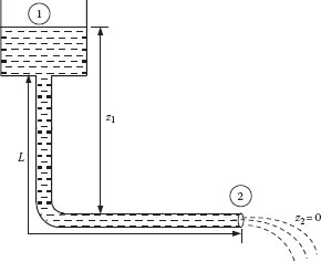
FIGURE E6.1 Slurry draining from a tank.
In order to get f, we must first calculate the Reynolds number
NRe = 4QρπDμ∞ = 4(9470 cm3/s)(1.8 g/cm3)π(7.62 cm)(0.85 g/cm s) = 3351
and the Hedstrom number
NHe = D2ρτoμ2∞ = (7.62 cm)2(1.8 g/cm3)(150 g/cm s2)(0.85 g/cm s)2 = 2420
Then we determine a from Equation 6.63
a = −1.47(1+0.146 exp [−2.9 × 10⁻⁵ NHe]) = −1.47(1+0.146 exp [−2.9 × 10⁻⁵(2420)]) = −1.670
and fL from Equation 6.60
fL ≈ 16NRe [1 + NHe8 NRe] = 163351 [1 + 24208(3351)] = 0.00521
Then we obtain fT from Equation 6.63
fT = 10aN0.193Re = 10−1.67033510.193 = 0.00446
m is found from Equation 6.66
m = 1.7 + 40,000NRe = 1.7 + 40,0003,351 = 13.64
And finally, we solve for f from Equation 6.65
f = (fmL + fmT)1/m = (0.0052113.64 + 0.0044613.64)1/13.64 = 0.00525
Now, we can determine the friction loss from Equation 6.68
ef = 32fLQ2π2D5 = 32(0.00525)(12,300 cm)(9,470 cm3/s)2π2(7.62 cm)5 = 7.31 × 105 cm2/s2
With regard to the kinetic energy terms in the Bernoulli equation, we may assume that the velocity in the tank is negligible compared to that in the pipe, that is, v1 ≪ v2. We will also neglect the kinetic energy of the stream leaving the pipe, as well as the friction loss in the contraction from the tank to the pipe, and any fittings such as elbows (these items may not be always negligible, however, and methods for evaluating them will be given in Chapter 7).
We may now solve the Bernoulli equation for the unknown z1:
z1 = efg + z2 = 7.31 × 10⁵ (cm2/s2)980 cm/s2 + 0 = 746 cm = 7.46 m
However, this vertical elevation will provide the required flow rate through only 115.4 m of horizontal pipe (and 7.46 m of vertical pipe). In order to provide the desired flow rate through 123 m of horizontal pipe, the desired elevation can be obtained by a simple ratio because the friction loss is a linear function of pipe length:
z123 = z115 (123115.4) = 7.46 m (123115.4) = 7.95 m
In this case, the flow rate is to be determined when a given fluid is transported in a given pipe with a known net driving force (e.g., pump head, pressure head, and/or hydrostatic head). The same total variables are involved as before, and hence the dimensionless variables are the same and are related in the same way as for the unknown driving force problems. The main difference is that now the unknown (Q) appears in two of the dimensionless variables (f and NRe), which requires a different solution strategy.
The problem statement is as follows:
Given: DF, D, L, ε, μ, ρ Find: Q
The strategy is to redefine the relevant dimensionless variables by combining the original groups in such a way that the unknown variable appears in one group. For example, f and NRe can be combined to eliminate the unknown (Q) as follows:
fN2Re = [DF π2D532LQ2] [4QρπDμ]2 = DFρ2D32Lμ2 |
(6.74) |
Thus, if we work with the three dimensionless variables fN2Re
There are various approaches that we can take to solve this problem. Since the Reynolds number is unknown, an explicit solution is not possible using the established relations between the friction factor and Reynolds number (e.g., the Moody diagram or Churchill equation). We can, however, proceed by a trial-and-error method that requires an initial guess for an unknown variable, use the basic relations to solve for this variable, revise the guess accordingly, and repeat the process (iterating) until agreement between calculated and guessed values is achieved.
Note that in this context, either f or NRe can be considered the unknown dimensionless variable because they both involve the unknown Q. As an aid in making the choice between these, a glance at the Moody diagram shows that the practical range of possible values of f is approximately one order of magnitude, whereas the corresponding possible range of NRe values is over five orders of magnitude. Thus, the chances of our initial guess being close to the final answer are greatly enhanced if we choose to iterate on f instead of NRe. Using this approach, the procedure is as follows:
1. A reasonable guess might be based on the assumption that the flow conditions are turbulent, for which the Colebrook equation, Equation 6.38, applies.
2. Calculate the value of fN2Re
3. Calculate f using the Colebrook equation, Equation 6.38.
4. Calculate NRe = (fN2Re/f)1/2
5. Using the value of NRe from step 4 and the known value of ε/D, determine f from the Moody diagram or Churchill equation (if NRe < 2000, use f = 16/NRe).
6. If this value of f does not agree with that from step 3, insert the value of f from step 5 into step 4 to get a revised value of NRe.
7. Repeat steps 5 and 6 until f no longer changes.
8. Calculate Q = πDμNRe/4ρ.
The problem statement is as follows:
Given: DF, D, L, m, n, ρ Find: Q
The simplest approach for this problem is also an iteration procedure, based on an assumed value of f:
1. A reasonable starting value for f is 0.005 based on a “dart throw” at the (equivalent) Moody diagram.
2. Calculate Q from Equation 6.68:
(6.75) |
3. Calculate the Reynolds number from Equation 6.71,
NRe, pl = (27−3nmπ2−n) ρQ2−nD4−3n (n3n + 1)n. |
(6.76) |
4. Calculate f from Equation 6.47.
5. Compare the values of f from step 4 and step 1. If they do not agree, use the result of step 4 in step 2 and repeat steps 2 through 5 until agreement is reached. Convergence usually requires only two or three trials, at most, unless very unusual conditions are encountered.
Example 6.2 Unknown Flow Rate of a Power Law Slurry
It is desired to determine the flow rate in gpm that would result for a slurry (ρ = 1.6 g/cm3) being pumped through a 300 ft long 2 in. ID pipe, with a pump that develops a discharge pressure of 85 psig. The pressure entering the pump is 10 psig, and the pipe discharges into a tank at atmospheric pressure. The slurry is characterized as a power law fluid with the properties m = 0.6 dyn sn/cm2 and n = 0.8 (Figure E6.2).
Solution:
The system parameters and fluid properties are listed here. We convert the data to cgs units for ease of manipulation:
Slurry consistency (m) = 0.6 (dyn sn/cm2) = 0.6 g/(cm s1.2)Slurry flow index (n) = 0.8Slurry density = 1.6 g/cm3Pump pressure = −ΔP = (85 psi) (atm/14.696 psi)(1.013 × 10⁶ dyn/[cm2 atm]) = 5.86 × 10⁶ dyn/cm2DF = −Δ P/ρ = (5.86 × 10⁶ dyn/cm2(g cm/s2 dyn)/(1.6 g/cm3) = 3.66 × 106 cm2/s2)L = 300 ft (30.48 cm/ft) = 9144 cmD = 2 in. (2.54 cm/in.) = 5.08 cmAssume f = 0.005.
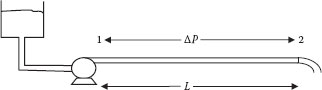
FIGURE E6.2 Unknown flow rate of power law fluid.
Calculate Q from Equation 6.68:
Q = π (D5DF32fL)1/2 = π [(5.08 cm)5(3.66× 106 cm2/s2)32(0.005)(9144 cm)]1/2 = 9142 cm3/s
Calculate the Reynolds number from Equation 6.71:
NRe, pl= (27−3nmπ2−n) ρQ2−nD4−3n (n3n+1)n= (27−3(0.8)0.6π2−(0.8)) (cm s1.2g) (0.83(0.8)+1)0.8 ((1.6 g/cm3)(9,142 cm3/s)2−0.8(5.08 cm)4−3(0.8)) = 21,641
Using Equations 6.48 to 6.51:
fL = 16NRe, pl = 1621,641 = 0.000739 |
(6.48) |
fT = 0.0682n−1/2N1/(1.87+2.39n)Re, pl = 0.0682(0.8)−0.5(21,641)1/(1.87+2.39(0.8)) = 0.00544 |
(6.50) |
α is given by
(6.51) |
where
Δ = NRe, pl − NRe, pl = 21,641 − 2,275 = 19,366
and
NRe, plc = 2100 + 875(1−n) = 2100 + 875(1−0.8) = 2275
Calculate f from Equation 6.47:
f = (1−α)fL + α[f−8T + f−8Tr]1/8 = 1[0.00544−8 + 0.0712−8]1/8 = 0.00544 |
(6.47) |
Repeat calculations with f = 0.00544 in place of 0.005 in Equation 6.68:
Q2 = Q(ff2)1/2 = 9142 cm3/s (0.0050.00544)1/2 = 8761 cm3/s
(NRe, pl)2 = NRe, pl (Q2Q)2−n = 21,641 (8,7619,142)1.2 = 20,563
(fL)2 = fL (NRe, pl(NRe, pl)2) = 0.000739 (21,64120,563) = 0.000778
(ftr)2 = ftr [(NRe, pl)2NRe, pl](0.414+0.757n) = 0.07121 (20,56321,641)1.096 = 0.0676
(fT)2 = fT [NRe, pl(NRe, pl)2]1/(1.87+2.39n) = 0.00544 [21,64120,563]0.2464 = 0.00552
Δ2 = (NRe,pl)2 − NRe, plc = 20,563 − 2,275 = 18,288
α2 = 11+4−Δ = 11+4−18288 = 1
f2 = (1−α2)(fL)2 + α2[f−8T + f−8Tr]1/82
= (1−1) + 1[0.00552−8 + 0.0676−8]1/8 = 0.00552
This is close enough to the previous value of 0.0.00544, so that no additional calculations are needed. Thus, the flow rate of 8761 cm3/s = 139 gpm
The procedure is very similar to the one that above.
Given: DF, D, L, μ∞, τo, ρ Find: Q
1. Assume f = 0.005.
2. Calculate Q from Equation 6.75.
3. Calculate the Reynolds and Hedstrom numbers:
NRe = 4QρπDμ∞, NHe = D2ρτoμ2∞. |
(6.77) |
4. Calculate f from Equation 6.65.
5. Compare the value of f from step 4 with the assumed value in step 1. If they do not agree, use the value of f from step 4 in step 2 and repeat steps 2 through 5 until they agree.
In this problem, it is desired to determine the size of the pipe (D) that will transport a given fluid (Newtonian or non-Newtonian) at a given flow rate (Q) over a given distance (L) with a given driving force (DF). Because the unknown (D) appears in each of the dimensionless variables, it is appropriate to regroup these variables in a more convenient form for this problem.
The problem statement is as follows:
Given: DF, Q, L, ε, ρ, μ Find: D
We can eliminate the unknown (D) from two of the three basic groups (NRe, ε/D, and f) as follows:
fN5Re = (DFπ2 D532LQ2) (4QρπDμ)5 = 32DFρ5Q3π3Lμ5 |
(6.78) |
(6.79) |
Thus, the three basic groups for this problem are fN5Re
1. Calculate fN5Re
2. Assume f = 0.005.
3. Calculate NRe from
(6.80) |
4. Calculate D from NRe:
(6.81) |
5. Calculate ε/D.
6. Determine f from the Moody diagram or Churchill equation using these values of NRe and ε/D (if NRe < 2000, use f = 16/NRe).
7. Compare the value of f from step 6 with the assumed value in step 2. If they do not agree, use the result of step 6 for f in step 3 in place of 0.005 and repeat steps 3 through 7 until they agree.
The problem statement is as follows:
Given: DF, Q, m, n, ρ, L Find: D
The procedure is analogous to that for the Newtonian fluid. In this case, the combined group fN5/(4−3n)Re, pl
The following procedure can be used to find D:
1. Calculate K from Equation 6.82:
fN5/(4−3n)Re, pl = (π2DFD532LQ2) [27−3n ρQ2−nD4−3n mπ2−n (n3n+1)n]5/(4−3n) = K |
(6.82) |
2. Assume f = 0.005.
3. Calculate NRe, pl from
(6.83) |
using f = 0.005.
4. Calculate f from Equation 6.47, using the value of NRe, pl from step 3.
5. Compare the result of step 4 with the assumed value in step 2. If they do not agree, use the value of f from step 4 in step 3, and repeat steps 3 through 5 until they agree. The diameter D is obtained from the last (converged) value of NRe, pl from step 3:
D = [27−3n ρQ2−nmπ2−n NRe, pl (n3n+1)n]1/(4−3n) |
(6.84) |
The problem variables are as follows:
Given: DF, Q, μ∞, τo, ρ, L Find: D
The combined group that is independent of D is equivalent to Equation 6.78, that is,
fN5Re = (D5π2DF32LQ2) (4Qρdπμ∞)5 = (32DFQ3ρ5π3Lμ5∞) |
(6.85) |
The following procedure can be used to find D:
1. Calculate fN5Re
2. Assume f = 0.01.
3. Calculate NRe from
(6.86) |
4. Calculate D from
(6.87) |
5. Calculate NHe from
(6.88) |
6. Calculate f from Equation 6.65 using the values of NRe and NHe from steps 3 and 5.
7. Compare the value of f from step 6 with the assumed value in step 2. If they do not agree, insert the result of step 6 for f into step 3 in place of 0.01, and repeat steps 3 through 7 until they agree.
The resulting value of D is determined in step 4.
Example 6.3 Unknown Diameter for a Newtonian Fluid
The flow configuration is the same as for Example 6.2 (see Figure E6.2).
In this case, the flow rate is given and it is desired to determine the pipe diameter that will deliver 600 gpm of water at 60°F with the given pump.
Solution:
The known quantities are listed here. We will assume that the pump in Example 6.2 operates the same on water as it does with the slurry, so that the pressure developed by the pump is the same. However, this is NOT a good assumption, as pumps designed to pump slurries are normally significantly different from those designed for clear liquids and have different performance characteristics. Nevertheless, we make this assumption here for the sake of simplicity.
Pump pressure = − ΔP = (85 psi)(atm/14.696 psi)(1.013 × 10⁶ dyn/[cm2atm]) = 3.66 × 10⁶ dyn/cm2
DF = −ΔP/ρ = (3.66 × 10⁶ dyn/cm2)(g cm/s2dyn)/(1 g/cm3) = 3.66 × 106 cm2/s2
L = 300 ft (30.48 cm/ft) = 9 144 cm
ε = 0.0018 in. = 0.00457 cm
Q = 600 gpm = (600 gpm)(63.09 cm3/(s gpm)) = 37,860 cm3/s
μ = 1 cP = 0.01 P = 0.01 dyn s/cm2 = 0.01 g/cm s
ρ = 1 g/cm3
1. Calculate fN5Re
2. Assume f = 0.005.
3. Calculate NRe from
NRe = (fN5Re0.005)1/5 = (2.151× 10260.005)1/5 = 5.33 × 10⁵
4. Calculate D from NRe:
D = 4QρπμNRe = 4(37, 850 cm3/s)(1g/cm3)π(0.01g/cm s) 5.33 × 105 = 9.04 cm |
(6.81) |
5. Calculate ε/D = 0.00457/9.04 = 5.06 × 10⁻⁴.
6. Determine f from the Churchill equation using the aforementioned values f = 0.0044.
Use this value in step 3, and revise the answer:
NRe2 = NRe1(f1f2)1/5 = 5.33 × 10⁵ (0.0050.0044)1/5 = 5.46 × 10⁵
Calculate D2 from NRe2:
D2 = 4QρπμNRe2 = 4(37,850 cm3/s)(1g/cm3)π(0.01g/cm s)5.46 × 105 = 8.83 cm = 3.50 in.ε/D = 0.00457/8.83 = 5.18 × 10⁻⁴
This gives basically the same value of f from the Churchill equation, so the answer is D = 8.83 cm or 3.50 in. It is not reasonable to expect standard commercial pipe to have the exact ID as calculated, so we would choose the pipe with the closest ID that would withstand the maximum pressure (which is 85 psig and small enough that any schedule pipe diameter should suffice). Actually, consulting the commercially available steel pipe dimensions (see Appendix F), we see that 3½ sch 40s pipe has an ID very close to that required here (3.55 in.). If this were not the case, we would choose the commercial pipe with the next larger standard ID for this system.
The relationship between flow rate, pressure drop, and pipe diameter for water flowing at 60°F in sch 40 horizontal pipe is tabulated in Appendix G over a range of pipe velocities that cover the most common conditions. For this special case, no iteration or other calculation procedures are required for any of the unknown driving force, unknown flow rate, or unknown diameter problems (although interpolation in the table is usually necessary). Note that the friction loss is tabulated in this table as pressure drop (in psi) per 100 ft of pipe, which is equivalent to (100 ρef/144 L) in the Bernoulli equation, where ρ is in (lbm/ft3), ef is in (ft lbf/lbm), and L is in (ft).
VII. TUBE FLOW (POISEUILLE) VISCOMETER
In Section II.B of Chapter 3, the tube flow viscometer was described in which the viscosity of any fluid with unknown viscous properties could be determined from measurements of the total pressure gradient (−ΔΦ/L) and the volumetric flow rate (Q) in a tube of known dimensions. The viscosity is given by
(6.89) |
where τw follows directly from the pressure gradient and Equation 6.4 and the wall shear rate is given by
(6.90) |
where
Γ = 4 Q/π R3 = 8V/D and
n′ = d log τwd log Γ = d log ΔΦd log Q |
(6.91) |
is the point slope of −ΔΦ versus Q at each measured value of Q. Equation 6.90 is completely independent of the specific fluid viscous properties and can be derived from Equation 6.7 as follows. By using Equation 6.4, the independent variable in Equation 6.7 can be changed from r to τrx, that is,
Q = −π R∫0r2˙γ dr = πR3τw τw∫0τ2rx ˙γ dτrx |
(6.92) |
This can be solved for the shear rate at the tube wall (˙γw)
(6.93) |
where Γ = 4Q/πR3. Solving for ˙γw
˙γw = 14τ2w d(Γτ3w)dτw = τw4 [dΓdτw + 3Γτw] = Γ(3n′ + 14n′) |
(6.94) |
where n′ = d(log τw)/d(log Γ) is the local slope of the log-log plot of τw versus Γ (or −ΔΦ vs Q) at each measured value of Q.
VIII. TURBULENT DRAG REDUCTION
A remarkable effect was observed by Toms during World War II when pumping NAPALM (a “jellied” solution of a polymer in gasoline). He found that the polymer solution could be pumped through pipes in turbulent flow with considerably lower pressure drop (friction loss) than that exhibited by the gasoline at the same flow rate in the same pipe without the polymer. This phenomenon, known as turbulent drag reduction (or the Toms effect), has been observed for solutions (mostly aqueous) of a variety of very high polymers (e.g., molecular weights on the order of 106) and has been the subject of a large amount of research. The effect is very significant because as much as 85% less energy is required to pump solutions of some high polymers at concentrations of 100 ppm or less through pipes than is required to pump the solvent alone at the same flow rate through the same pipe. This is illustrated in Figure 6.5, which shows some of Chang’s data (Darby and Chang, 1984) for the Fanning friction factor versus Reynolds number (based on the solvent viscosity) for fresh and “degraded” polyacrylamide solutions of concentrations from 100 to 500 ppm in a 2 mm diameter tube. Note that the friction factor at low Reynolds numbers (laminar flow) is much larger than that for the (Newtonian) solvent, whereas it is much lower at high (turbulent) Reynolds numbers. The non-Newtonian viscosity of these solutions is shown in Figure 3.9 in Chapter 3.
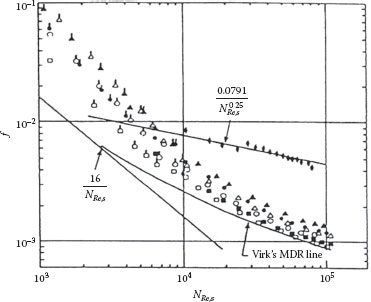
FIGURE 6.5 Drag reduction data for polyacrylamide solutions (NRe, s is the Reynolds number based on solvent properties.) MDR is Virk’s maximum drag reduction asymptote (Virk, 1975). (From Darby, R. and Chang, H.D., AIChE J., 30, 274, 1984.)
Although the exact mechanism is debatable, Darby and Chang (1984) and Darby and Pivsa-Art (1991) have presented a model for turbulent drag reduction based on the fact that solutions of very high molecular weight polymers are viscoelastic and the concept that in any unsteady deformation (such as turbulent flow) elastic properties will store energy that would otherwise be dissipated in a purely viscous fluid. Since energy that is dissipated (i.e., the “friction loss”) must be made up by adding energy (e.g., by a pump) to sustain the flow, that portion of the energy that is stored by elastic deformations remains in the flow and does not have to be made up by external energy sources. Thus, less energy must be supplied externally to sustain the flow of a viscoelastic fluid, that is, the drag is reduced. This concept is analogous to that of bouncing an elastic ball. If there is no viscosity (i.e., internal friction) to dissipate the energy, the ball will continue to bounce indefinitely with no external energy input needed. However, a viscous ball will not bounce at all, because all of the energy is dissipated by viscous deformation upon contact with the floor and is transformed into “heat.” Thus, the greater the fluid elasticity in proportion to the viscosity, the lesser the amount of energy that must be added to replace that which is dissipated by the turbulent motion of the flow.
The model for turbulent drag reduction developed by Darby and Chang (1984) and later modified by Darby and Pivsa-Art (1991) shows that for smooth tubes the friction factor versus Reynolds number relationship for Newtonian fluids (e.g., the Colebrook or Churchill equation) may also be used for drag reducing flows, provided (1) the Reynolds number is defined using the properties (e.g., viscosity) of the Newtonian solvent and (2) the Fanning friction factor is modified as follows:
(6.95) |
where
fs is the solvent (Newtonian) Fanning friction factor as predicted for a Newtonian fluid with the viscosity of the solvent using the (Newtonian) Reynolds number
fp is a “generalized” Fanning friction factor that applies to drag reducing polymer solutions as well as Newtonian fluids
NDe is the dimensionless Deborah number, which depends upon the fluid viscoelastic properties and accounts for the storage of energy by the elastic deformations
The replotted data are well represented by the classic Colebrook equation shown as the line on this plot. Figure 6.6 shows the data from Figure 6.5 (and many other data sets as well) replotted in terms of the generalized friction factor.
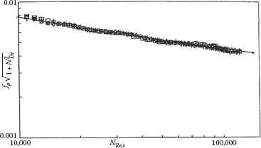
FIGURE 6.6 Drag reduction data replotted in terms of generalized friction factor. (From Darby, R. and Pivsa-Art, S., Canad. J. Chem. Eng., 69, 1395, 1991.)
The complete expression for NDe is given by Darby and Pivsa-Art (1991) as a function of the viscoelastic properties of the fluid (i.e., the Carreau parameters ηo, λ, and p). This expression is as follows:
NDe = 0.0163NςN0.338Re, s (μs/ηo)0.5[1/N0.75Re,s + 0.00476N2ς(μs/ηo)0.75]0.318 |
(6.96) |
where
(6.97) |
and
(6.98) |
where
NRe, s is the Reynolds number based on the solvent properties
μs is the solvent viscosity
D is the pipe diameter
V is the velocity in the pipe
λ is the fluid time constant (from the Carreau model fit of the viscosity curve)
Inasmuch as the rheological properties are very difficult to measure for very dilute solutions (e.g., 100 ppm or less), a simplified expression was developed by Darby and Pivsa-Art (1991) in which these rheological parameters are contained within two “constants,” k1 and k2:
NDe = k2 (8μsNRe, sρD2)k1 N0.34Re, s |
(6.99) |
where k1 and k2 depend only on the specific polymer solution and its concentration. Darby and Pivsa-Art (1991) examined a variety of drag reducing data sets from the literature for various polymer solutions in various size pipes and determined the corresponding values of k1 and k2 that fit the model to the data. These values are given in Table E6.1.
For any drag reducing solution, k1 and k2 can be determined experimentally from two data points in the laboratory at two different flow rates (i.e., Reynolds numbers) in turbulent flow in any size pipe. The resulting values can be used with the model to predict friction loss for that solution at any Reynolds number in any size pipe. If the Colebrook equation for smooth tubes is used, for example, the appropriate generalized expression for the friction factor is
f = 0.41[ln(NRe,s/7)]2 1(1 + N2De)1/2 |
(6.100) |
Parameters for Equation 6.99 for Various Polymer Solutions
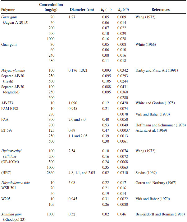
Source: Darby, R. and Pivsa-Art, S., Canad. J. Chem. Eng., 69, 1395, 1991.
Example 6.4 Friction Loss in Drag Reducing Solutions
Determine the percentage reduction in the power required to pump water through a 3 in. ID smooth pipe at 300 gpm by adding 100 wppm of “degraded” Separan AP-30.
Solution:
We first calculate the Reynolds number for the solvent (water) under the given flow conditions using a viscosity of 0.01 poise and a density of 1 g/cm3:
NRe, s = 4QρπDμ = 4(300 gpm)[63.1 cm3/s gpm](1g/cm3)π(3 in.)(2.54 cm/in.)(0.01 g/cm s) = 3.15 × 10⁵
Then calculate the Deborah number from Equation 6.99 using k1 = 0.088 and k2 = 0.0431 taken from Table E6.1:
NDe = k2(8μsNRe, sρD2)k1 N0.34Re, s = 0.0431 (8 × 0.01(g/cm s)× 3.15 × 1051(g/cm3) × (3 in. × 2.54 (cm/in.))2)0.088 (3.15 × 10⁵)0.34 = 5.45
These values can now be used to calculate the smooth pipe friction factor from Equation 6.100. Excluding the NDe term gives the friction factor for the Newtonian solvent (fs), and including the NDe term gives the friction factor for the polymer solution (fp) under the same flow conditions:
fs = 0.41[ln (NRe, s/7)]2 = 0.00357
fp = 0.41[ln (NRe, s/7)]2 1(1+N2De) = 0.000645
The power (HP) required to pump the fluid is given by −ΔPQ. Because −ΔP is proportional to fQ2 and Q is the same with and without the polymer, the fractional reduction in power is given by
DR = HPs − HPpHPs = fs − fpfs = (0.00357 − 0.000645)/0.00357 = 0.82
That is, adding the polymer results in an 82% reduction in the power required to overcome drag.
This chapter contains all of the fundamental information and methods for solving virtually any kind of problem involving pipe flows under any and all conditions and for a wide variety of fluids. The major concepts that should be retained from this chapter include the following:
• Understand the principles governing the flow of Newtonian and non-Newtonian in pipes, including the application of the momentum and energy balances (and the similarity thereof).
• Understand the concepts governing turbulent flow, the models that describe turbulent pipe flow, and applications including turbulent drag reduction.
• Be able to solve for either the unknown driving force or the unknown flow rate or the unknown diameter in pipes for Newtonian and non-Newtonian fluids.
PIPE FLOWS
1. Show how the Hagen–Poiseuille equation for the steady laminar flow of a Newtonian fluid in a uniform cylindrical tube can be derived starting from the general microscopic equations of motion (e.g., the continuity and momentum equations given in Appendix E).
2. The Hagen–Poiseuille equation (Equation 6.11) describes the laminar flow of a Newtonian fluid in a tube. Since a Newtonian fluid is defined by the relation τ = μ˙γ
3. Derive the relation between the friction factor and Reynolds number in turbulent flow for smooth pipe (Equation 6.34), starting with the von Karman equation for the velocity distribution in the turbulent boundary layer (Equation 6.26).
4. Evaluate the kinetic energy correction factor α in the Bernoulli equation for turbulent flow assuming the 1/7 power law velocity profile (Equation 6.36) is valid. Repeat this for laminar flow of a Newtonian fluid in a tube, for which the velocity profile is parabolic.
5. A Newtonian fluid with SG = 0.8 is forced through a capillary tube at a rate of 5 cm3/min. The tube has a downward slope of 30° to the horizontal, and the pressure drop is measured between two taps located 40 cm apart on the tube using a mercury manometer, which reads 3 cm. When water is forced through the tube at a rate of 10 cm3/min, the manometer reading is 2 cm.
(a) What is the viscosity of the unknown Newtonian fluid?
(b) What is the Reynolds number of the flow for each fluid?
(c) If two separate pressure transducers, which read the total pressure directly in psig, were used to measure the pressure at each of the pressure taps directly instead of using the manometer, what would be the difference in the transducer readings?
6. A liquid is draining from a cylindrical vessel through a tube in the bottom of the vessel, as illustrated in Figure P6.6 below. If the liquid has a specific gravity of 0.85 and drains out at a rate of 1 cm3/s, what is the viscosity of the liquid? The entrance loss coefficient from the tank to the tube is 0.4, and the system has the following dimensions: D = 2 in., d = 2 mm, L = 10 cm, and h = 5 cm
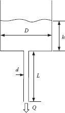
FIGURE P6.6 Fluid draining through tube.
7. You are given a liquid and are asked to find its viscosity. Its density is known to be 0.97 g/cm3. You place the fluid in an open vessel to which a 20 cm long vertical tube with an inside diameter of 2 mm is attached to the bottom (see Figure P6.6). When the depth of the liquid in the container is 6 cm, you find that it drains out through the tube at a rate of 2.5 cm3/s. If the diameter of the open vessel is much larger than that of the tube and friction loss from the vessel to the tube is negligible, what is the fluid viscosity?
8. Repeat problem 7 accounting for the friction loss from the vessel to the tube, assuming a loss coefficient of 0.50 at the contraction.
9. You must measure the viscosity of an oil that has an SG of 0.92. To do this, you put the oil into a large container to the bottom of which a small vertical tube, 25 cm long, has been attached through which the oil can drain by gravity (see Figure P6.6). When the level of the oil in the container is 6 in. above the container bottom, you find that the flow rate through the tube is 50 cm3/min. You run the same experiment with water instead of oil and find that under the same conditions the water drains out at a rate of 156 cm3/min. If the loss coefficient for the energy dissipated in the contraction from the container to the tube is 0.5, what is the viscosity of the oil?
10. You want to transfer No. 3 fuel oil (30°API) from a storage tank to a power plant at a rate of 2000 bbl/day. The diameter of the pipeline is 1½ in. sch 40, with a length of 1200 ft. The discharge of the line is 20 ft higher than the suction end, and both ends are at 1 atm pressure. The inlet temperature of the oil is 60°F, and the transfer pump is 60% efficient. If the specific heat of the oil is 0.5 Btu/(lbm° F) and the pipeline is perfectly insulated, determine
(a) The horsepower of the motor required to drive the pump
(b) The temperature of the oil leaving the pipeline
11. You must specify a pump to deliver 800 bbl/day of a 35° API distillate at 90°F from a distillation column to a storage tank in a refinery. If the level in the tank is 20 ft above that in the column, the total equivalent length of pipe is 900 ft, and both the column and tank are at atmospheric pressure, what horsepower would be needed if you use 1½ in. sch 40 pipe? What power would be needed if you use 1 in. sch 40 pipe?
12. Water is flowing at a rate of 700 gpm through a horizontal 6 in. sch 80 commercial steel pipe at 90°F. If the pressure drops by 2.23 psi over a 100 ft length of pipe, determine the following:
(a) What is the value of the Reynolds number?
(b) What is the magnitude of the pipe wall roughness?
(c) How much driving force (i.e., pressure difference) would be required to move the water at this flow rate through 10 miles of pipe if it were made of commercial steel?
(d) What size commercial steel pipe would be required to transport the water at the same flow rate over the same distance if the driving force is the static head in a water tower 175 ft above the pipe?
13. A 35° API distillate at 60°F is to be pumped over a distance of 2000 ft through a 4 in. sch 40 horizontal pipeline at a flow rate of 500 gpm. What power must the pump deliver to the fluid if the pipeline is made of (a) drawn tubing, (b) commercial steel, (c) galvanized iron, and (d) PVC plastic?
14. The Moody diagram illustrates the effect of roughness on the friction factor in turbulent flow but indicates no effect of roughness in laminar flow. Explain why this is so. Are there any restrictions or limitations that should be placed on this conclusion? Explain.
15. You have a large supply of very rusty 2 in. sch 40 steel pipe, which you want to use for a pipeline. Because rusty metal is rougher than clean metal, you want to know its effective roughness before laying the pipeline. To do this, you pump water at a rate of 100 gpm through a 100 ft long section of the pipe and find that the pressure drops by 15 psi over this length. What is the effective pipe roughness in inches?
16. A 32 hp pump (100% efficient) is required to pump water through a 2 in. sch 40 pipeline, 6000 ft long, at a rate of 100 gpm.
(a) What is the equivalent roughness of the pipe?
(b) If the pipeline is replaced by new commercial steel 2 in. sch 40 pipe, what power would be required to pump water at a rate of 100 gpm through this pipe? What would be the percentage saving in power compared to the old pipe?
17. You have a piping system in your plant that has gotten old and rusty. The pipe is 2 in. sch 40 steel, 6000 ft long. You find that it takes 35 hp to pump water through the system at a rate of 100 gpm.
(a) What is the equivalent roughness of the pipe?
(b) If you replace the pipe with the same size new commercial steel pipe, what percentage savings in the required power would you expect at a flow rate of 100 gpm?
18. Water enters a horizontal tube through a flexible vertical rubber hose that can support no forces. If the tube is 1/8 in. sch 40, 10 ft long, and the water flow rate is 2 gpm, what force (magnitude and direction) must be applied to the tube to keep it stationary? Neglect the weight of the tube and the water in it. The hose ID is the same as that of the tube.
19. A water tower that is 90 ft high provides water to a residential subdivision. The water main from the tower to the subdivision is 6 in. sch 40 steel, 3 miles long. If each house uses a maximum of 50 gal/h (at peak demand) and the pressure in the water main is not to be less than 30 psig at any point, how many homes can be served by the water main?
20. A heavy oil (μ = 100 cP, SG = 0.85) is draining from a large tank through a 1/8 in. sch 40 tube into an open bucket. The level in the tank is 3 ft above the tube inlet, and the pressure in the tank is 10 psig. The tube is 30 ft long, and it is inclined downward at an angle of 45° to the horizontal. What is the flow rate of the oil in gpm? What is the value of the Reynolds number in this problem?
21. SAE 10 lube oil (SG = 0.93) is being pumped upward through a straight 1/4 in. sch 80 pipe that is oriented at 45° angle to the horizontal. The two legs of a manometer using water as the manometer fluid are attached to taps in the pipe wall that are 2 ft apart. If the manometer reads 15 in., what is the oil flow rate in gal/h?
22. Cooling water is fed by gravity from an open storage tank 20 ft above ground, through 100 ft of 1½ in. ID steel pipe, to a heat exchanger at ground level. If the pressure entering the heat exchanger must be 5 psig for it to operate properly, what is the water flow rate through the pipe?
23. A water main is to be laid to supply water to a subdivision located 2 miles from a water tower. The water in the tower is 150 ft above ground, and the subdivision consumes a maximum of 10,000 gpm of water. What size pipe should be used for the water main? Assume Schedule 40 commercial steel pipe. The pressure above the water in the tank is 1 atm and is 30 psig at the subdivision.
24. A water main is to be laid from a water tower to a subdivision that is 2 miles away. The water level in the tower is 150 ft above the ground. The main must supply a maximum of 1000 gpm with a minimum of 5 psig at the discharge end, at a temperature of 65°F. What size commercial steel sch 40 pipe should be used for the water main? If plastic pipe (which is hydraulically smooth) were used instead, would this alter the result? If so, what diameter of plastic pipe should be used?
25. The water level in a water tower is 110 ft above ground level. The tower supplies water to a subdivision, 3 miles away, through an 8 in. sch 40 steel water main. If the minimum water pressure entering the residential water lines at the houses must be 15 psig, what is the capacity of the water main (in gpm)? If there are 100 houses in the subdivision and each consumes water at a peak rate of 20 gpm, how big should the water main be?
26. A hydraulic press is powered by a remote high-pressure pump. The gage pressure at the pump is 20 MPa, and the pressure required to operate the press is 19 MPa (gage) at a flow rate of 0.032 m3/min. The press and pump are to be connected by 50 m of drawn stainless steel tubing. The fluid properties are those of SAE 10 lube oil at 40°C. What is the minimum tubing diameter that can be used?
27. Water is to be pumped at a rate of 100 gpm from a well that is 100 ft deep, through 2 miles of horizontal 4 in. sch 40 steel pipe, to a water tower that is 150 ft high.
(a) Neglecting fitting losses, what horsepower will the pump require if it is 60% efficient?
(b) If the elbow in the pipe at ground level below the tower breaks off, how fast will the water drain out of the tower?
(c) How fast would it drain out if the elbow at the top of the well gave way instead?
(d) What size pipe would you have to run from the water tower to the ground in order to drain it at a rate of 10 gpm?
28. A concrete pipe storm sewer, 4 ft in diameter, drops 3 ft in elevation per mile of length. What is the maximum capacity of the sewer (in gpm) when it is flowing full?
29. You want to siphon water from an open tank using a 1/4 in. diameter hose. The discharge end of the hose is 10 ft below the water level in the tank, and the siphon will not operate if the pressure falls below 1 psia anywhere in the hose. If you want to siphon the water at a rate of 1 gpm, what is the maximum height above the water level in the tank that the hose can extend and still operate?
NON-NEWTONIAN PIPE FLOWS
30. Equation 6.43 describes the laminar flow of a power law fluid in a tube. Since a power law fluid is defined by the relation τ = m˙γn
31. A large tank contains SAE 10 lube oil at a temperature of 60°F and a pressure of 2 psig. The oil is 2 ft deep in the tank and drains out through a vertical tube in the bottom. The tube is 10 ft long and discharges the oil at atmospheric pressure. Assuming the oil to be Newtonian and neglecting the friction loss from the tank to the tube, how fast will it drain through the tube? If the oil is not Newtonian, but instead can be described as a power law fluid with a flow index of 0.4 and an apparent viscosity of 80 cP at a shear rate of 1 s−1, how would this affect your answer? The tube diameter is 1/2 in.
32. A polymer solution is to be pumped at a rate of 3 gpm through a horizontal 1 in. diameter pipe. The solution behaves as a power law fluid with a flow index of 0.5, an apparent viscosity of 400 cP at a shear rate of 1 s−1, and a density of 60 lbm/ft3.
(a) What is the pressure gradient in psi/ft?
(b) What is the shear rate at the pipe wall and the apparent viscosity of the fluid at this shear rate?
(c) If the fluid were Newtonian, with a viscosity equal to the apparent viscosity from (b) above, what would the pressure gradient be?
(d) Calculate the Reynolds numbers for the polymer solution and for the above Newtonian fluid.
33. A coal slurry that is characterized as a power law fluid has a flow index of 0.4 and an apparent viscosity of 200 cP at a shear rate of 1 s−1. If the coal has a specific gravity of 2.5 and the slurry is 50% coal by weight in water, what pump horsepower will be required to transport 25 million tons of coal per year through a 36 in. ID, 1000 miles long pipeline? Assume that the entrance and exit of the pipeline are at the same pressure and elevation and that the pumps are 60% efficient.
34. A coal slurry is found to behave as a power law fluid, with a flow index of 0.3, a specific gravity of 1.5, and an apparent viscosity of 70 cP at a shear rate of 100 s−1. What volumetric flow rate of this fluid would be required to reach turbulent flow in a 1/2 in. ID smooth pipe, which is 15 ft long? What is the pressure drop in the pipe (in psi) under these conditions?
35. A coal slurry is to be transported by pipeline. It has been determined that the slurry may be described by the power law model, with a flow index of 0.4, an apparent viscosity of 50 cP at a shear rate of 100 s−1, and a density of 90 lbm/ft3. What horsepower would be required to pump the slurry at a rate of 900 gpm through an 8 in. sch 40 pipe that is 50 miles long?
36. A sewage sludge is to be transported a distance of 3 mi through a 12 in. ID pipeline at a rate of 2000 gpm. The sludge is a Bingham plastic with a yield stress of 35 dyn/cm2, a limiting viscosity of 80 cP, and a specific gravity of 1.2. What size motor (in horsepower) would be required to drive the pump if it is 50% efficient?
37. A coal suspension is found to behave as a power law fluid, with a flow index of 0.4, a specific gravity of 1.5, and an apparent viscosity of 90 cP at a shear rate of 100 s−1. What would the volumetric flow rate of this suspension be in a 15 ft long, 5/8 in. ID smooth tube, with a driving force of 60 psi across the tube? What is the Reynolds number for the flow under these conditions?
38. A coal-water slurry containing 65% (by weight) coal is pumped from a storage tank at a rate of 15 gpm through a 50 m long 1/2 in. sch 40 pipeline to a boiler where it is burned. The storage tank is at 1 atm pressure and 80°F, and the slurry must be fed to the burner at 20 psig. The specific gravity of coal is 2.5, and it has a heat capacity of 0.5 Btu/(lbm° F).
(a) What power must the pump deliver to the slurry if it is assumed to be Newtonian with a viscosity of 200 cP?
(b) In reality, the slurry is non-Newtonian and can best be described as a Bingham plastic, with a yield stress of 800 dyn/cm2 and a limiting viscosity of 200 cP. Accounting for these properties, what would the required pumping power be?
(c) If the pipeline is well insulated, what will the temperature of the slurry be when it enters the boiler, for both case (a) and case (b)?
39. A sludge is to be transported by pipeline. It has been determined that the sludge may be described by the power law model, with a flow index of 0.6, an apparent viscosity of 50 cP at a shear rate of 1 s−1, and a density of 95 lbm/ft3. What hydraulic horsepower would be required to pump the sludge at a rate of 600 gpm through a 6 in. ID pipe that is 5 miles long?
40. You must design a transfer system to feed a coal slurry to a boiler. However, you don’t know the slurry properties, so you measure them in the lab using a cup and bob (Couette) viscometer. The cup has a diameter of 10 cm and a bob diameter of 9.8 cm, and the length of the bob is 8 cm. When the cup is rotated at a rate of 2 rpm, the torque measured on the bob is 2.4 × 10⁴ dyn cm, and at 20 rpm, it is 6.5 × 10⁴ dyn cm.
(a) If you use the Bingham plastic model to describe the slurry properties, what are the values of the yield stress and the limiting viscosity?
(b) If the power law model were used instead, what would be the values of the flow index and consistency?
(c) Using the Bingham plastic model for the slurry, with a value of the yield stress of 35 dyn/cm2, a limiting viscosity of 35 cP, and a density of 1.2 g/cm3, what horsepower would be required to pump the slurry through a 1000 ft long, 3 in. ID sch 40 pipe at a rate of 100 gpm?
41. A thick slurry with SG = 1.3 is to be pumped through a 1 in. ID pipe that is 200 ft long. You don’t know the properties of the slurry, so you test it in the lab by pumping it through a 4 mm ID tube that is 1 m long. At a flow rate of 0.5 cm3/s, the pressure drop in this tube is 1 psi, and at a flow rate of 5 cm3/s, it is 1.5 psi. Estimate the pressure drop that would be required to pump the slurry through the 1 in. pipe at a rate of 2 gpm and also at 30 gpm. Clearly explain the procedure you use, and state any assumptions that you make. Comment in detail about the possible accuracy of your predictions. The slurry SG is 1.3.
42. Drilling mud has to be pumped down into an oil well that is 8000 ft deep. The mud is to be pumped at a rate of 50 gpm to the bottom of the well and back to the surface, through a pipe having an effective ID of 4 in. The pressure at the bottom of the well is 4500 psi. What pump head is required to do this? The drilling mud has properties of a Bingham plastic, with a yield stress of 100 dyn/cm2, a limiting (plastic) viscosity of 35 cP, and a density of 1.2 g/cm3.
43. A straight vertical tube, 100 cm long and 2 mm ID, is attached to the bottom of a large vessel. The vessel is open to the atmosphere and contains a liquid with a density of 1 g/cm3 to a depth of 20 cm above the bottom of the vessel.
(a) If the liquid drains through the tube at a rate of 3 cm3/s, what is its viscosity?
(b) What is the largest tube diameter that can be used in this system to measure the viscosity of liquids that are at least as viscous as water, for the same liquid level in the vessel? Assume that the density is the same as water.
(c) A non-Newtonian fluid, represented by the power law model, is introduced into the vessel with the 2 mm diameter tube attached. If the fluid has a flow index of 0.65, an apparent viscosity of 5 cP at a shear rate of 10 s−1, and a density of 1.2 g/cm3, how fast will it drain through the tube, if the level is 20 cm above the bottom of the vessel?
44. A non-Newtonian fluid, described by the power law model, is flowing through a thin slit between two parallel planes of width W, separated by a distance H. The slit is inclined upward at an angle θ to the horizontal.
(a) Derive an equation relating the volumetric flow rate of this fluid to the pressure gradient, slit dimensions, and fluid properties.
(b) For a Newtonian fluid, this solution can be written in a dimensionless form as
f = 24/NRe, h
where the Reynolds number, NRe, h, is based on the hydraulic diameter of the channel. Arrange your solution for the power law fluid in dimensionless form and solve for the friction factor, f.
(c) Set your result from (b) equal to 24/NRe, h, and determine an equivalent expression for the power law Reynolds number for slit flow.
45. You are drinking a milk shake through a straw that is 8 in. long and 0.3 in. in diameter. The milk shake has the properties of a Bingham plastic, with a yield stress of 300 dyn/cm2, a limiting viscosity of 150 cP, and a density of 0.8 g/cm3.
(a) If the straw is inserted 5 in. below the surface of the milk shake, how hard must you suck to get the shake flowing through the entire straw (e.g., how much vacuum must you pull, in psi)?
(b) If you pull a vacuum of 1 psi, how fast will the shake flow (in cm3/s)?
46. Water is to be transferred at a rate of 500 gpm from a cooling lake through a 6 in. diameter sch 40 pipeline to an open tank in a plant that is 30 miles from the lake.
(a) If the transfer pump is 70% efficient, what horsepower motor is required to drive the pump?
(b) An injection station is installed at the lake that injects a high polymer into the pipeline to give a solution of 50 ppm concentration with the following properties: a low shear-limiting viscosity of 80 cP, a flow index of 0.5, and a transition point from low shear Newtonian to shear thinning behavior at a shear rate of 10 s−1. What horsepower is now required to drive the same pump to achieve the same flow rate?
47. You measure the viscosity of a sludge in the lab and conclude that it can be described as a power law fluid with a flow index of 0.45, a viscosity of 7 poise at a shear rate of 1 s−1, and a density of 1.2 g/cm3.
(a) What horsepower would be required to pump the sludge through a 3 in. sch 40 pipeline, 1000 ft long, at a rate of 100 gpm?
(b) The viscosity data show that the sludge could also be described by the Bingham plastic model, with a viscosity of 7 poise at a shear rate of 1 s−1 and a viscosity of 0.354 poise at a shear rate of 100 s−1. Using this model, what required horsepower would you predict for this pipeline?
(c) Which answer do you think would be the most reliable and why?
48. An open drum, 3 ft in diameter, contains a mud that is known to be described by the Bingham plastic model, with a yield stress of 120 dyn/cm2, a limiting viscosity of 85 cP, and a density of 98 lbm/ft3. A 1 in. ID hose, 10 ft long, is attached to a hole in the bottom of the drum to drain the mud out. How far below the surface of the mud should the end of the hose be lowered in order to drain the mud at a rate of 5 gpm?
49. You would like to determine the pressure drop–flow rate relation for a slurry in a pipeline. To do this, you must determine the rheological properties of the slurry, so you test it in the lab by pumping it through a 1/8 in. ID pipe that is 10 ft long. You find that it takes 5 psi pressure drop in the pipe to produce a flow rate of 100 cm3/s and that 10 psi results in a flow rate of 300 cm3/s.
(a) What can you deduce about the rheological characteristics of the slurry from these data?
(b) If it is assumed that the slurry can be adequately described by the power law model, what are the values of the fluid properties, as deduced from the data?
(c) If the Bingham plastic model is used instead of the power law model to describe the slurry, what are its properties?
50. A pipeline is installed to transport a red mud slurry from an open tank in an alumina plant to a disposal pond. The line is 5 in. sch 80 commercial steel, 12,000 ft long, and is designed to transport the slurry at a rate of 300 gpm. The slurry properties can be described by the Bingham plastic model, with a yield stress of 15 dyn/cm2, a limiting viscosity of 20 cP, and an SG of 1.3. You may neglect any fittings in this pipeline.
(a) What delivered pump head and hydraulic horsepower would be required to pump this mud?
(b) What would be the required pump head and horsepower to pump water at the same rate through the same pipeline?
(c) If 100 ppm of fresh Separan AP-30 polyacrylamide polymer were added to the water in case (b), what would the required pump head and horsepower be?
51. Determine the power required to pump water at a rate of 300 gpm through a 3 in. ID pipeline, 50 mi long, if
(a) The pipe is new commercial steel
(b) The pipe wall is hydraulically smooth
(c) The pipe wall is smooth, and “degraded” Separan AP-30 polyacrylamide is added to the water at a concentration of 100 wppm.
D |
Diameter, [L] |
DF |
“Driving Force,” Equation 6.67, [FL/M = L2/t2] |
ef |
Energy dissipated per unit mass of fluid, [FL/M = L2/t2] |
f |
Fanning friction factor, [—] |
Fx |
Force component in x direction, [F = ML/t2] |
Kf |
Loss coefficient, [—] |
L |
Length, [L] |
m |
Power law consistency parameter, [M/(Lt2−n)] |
n |
Power law flow index, [—] |
NBi |
Bingham number, [—] |
NDe |
Deborah number, [—] |
NHe |
Hedstrom number, Equation 6.62, [—] |
NRe |
Reynolds number, [—] |
NRe, s |
Solvent Reynolds number, [—] |
NRe, pl |
Power law Reynolds number, [—] |
P |
Pressure, [F/L2 = M/(Lt2)] |
Q |
Volumetric flow rate, [L3/t] |
r |
Radial direction, [L] |
R |
Tube radius, [L] |
t |
Time, [t] |
V |
Spatial average velocity, [L/t] |
v* |
Friction velocity, Equation 6.28, [L/t] |
vx |
Local velocity in the x direction, [L/t] |
v′x |
Turbulent eddy velocity component in the x direction, [L/t] |
v+ |
Dimensionless velocity, Equation 6.27, [—] |
w |
External shaft work (e.g., negative pump work) per unit mass of fluid, [FL/M = M/Lt2] |
y+ |
Dimensionless distance from wall, Equation 6.27, [—] |
GREEK
δL |
Laminar boundary layer thickness, [L] |
δT |
Turbulent boundary layer thickness, [L] |
ε |
Roughness, [L] |
Φ |
Potential = P + ρgz, [F/L2 = M/(Lt2)] |
μ |
Viscosity (constant), [M/(Lt)] |
ρ |
Density, [M/L3] |
τo |
Yield stress, [F/L2 = M/(Lt2)] |
τrx |
Shear stress component, force in x direction on r surface, [F/L2 = M/(Lt2)] |
τ′rx |
Turbulent (Reynolds) stress component, [F/L2 = M/(Lt2)] |
τw |
Stress exerted by the fluid on the wall, [F/L2 = M/(Lt2)] |
SUBSCRIPTS
x, y, z, r, θ |
Coordinate directions |
w |
Wall location |
Astarita, G., G. Greco Jr., and L. Nicodemo, A phenomenological interpretation and correlation of drag reduction, AIChE J., 15, 564–567, 1969.
Bewersdorff, H.W. and N.S. Berman, The influence of flow-induced non-Newtonian fluid properties on turbulent drag reduction, Rheol. Acta, 27, 130–136, 1988.
Churchill, S.W., Friction factor equation spans all fluid flow regimes, Chem. Eng., 84 (24), 91–92, November 7, 1977.
Darby, R. and H.D. Chang, Generalized correlation for friction loss in drag reducing polymer solutions, AIChE J., 30, 274–280, 1984.
Darby, R. and J. Melson, How to predict the friction factor for flow of Bingham plastics, Chem. Eng., 28, 59–61, 1981.
Darby, R., R. Mun, and D.V. Boger, Predicting friction loss in slurry pipelines, Chem. Eng., 99, 116–119, September 1992.
Darby, R. and S. Pivsa-Art, An improved correlation for turbulent drag reduction in dilute polymer solutions, Canad. J. Chem. Eng., 69, 1395–1400, 1991.
Dodge, D.W. and A.B. Metzner, Turbulent flow of non-Newtonian systems, AIChE J., 5, 189–204, 1959.
Goren, Y. and J.F. Norbury, Turbulent flow of dilute aqueous polymer solutions, ASME J. Basic Eng., 89, 814–822, 1967.
Hoffmann, L. and P. Schummer, Experimental investigation of the turbulent boundary layer in the pipe flow of viscoelastic fluids, Rheol. Acta, 17, 98–104, 1978.
Savins, J.G., Contrasts in the solution drag reduction characteristics of polymeric solutions and micellar systems, in Viscous Drag Reduction, C.S. Wells (Ed.), Plenum Press, New York, 1969, pp. 183–212.
Virk, P.S., Drag reduction fundamentals, AIChE J., 21, 625–656, 1975.
Virk, P.S. and H. Baher, The effect of polymer concentration on drag reduction, Chem. Eng. Sci., 25, 1183–1189, 1970.
Wang, C.B., Correlation of the friction factor for turbulent pipe flow of dilute polymer solutions, Ind. Eng. Chem. Fund., 11, 546–551, 1972.
White, A., Turbulent drag reduction with polymer additives, J. Mech. Eng. Sci., 8, 452–455, 1966.
White, D. Jr. and R.J. Gordon, The influence of polymer conformation on turbulent drag reduction, AIChE J., 21, 1027–1029, 1975.
* Leibnitz rule:
∂∂x B(x)∫A(x)I(x, y)dy = B(x)∫A(x)∂I∂x dy + I(x, B) ∂B∂x − I(x, A) ∂A∂x.