Chapter 9
Summarizing Sheets
IN THIS CHAPTER
![]() Creating new spreadsheets
Creating new spreadsheets
![]() Entering and formatting numbers
Entering and formatting numbers
![]() Using Sheets to calculate
Using Sheets to calculate
![]() Saving, exporting, and collaborating with Sheets
Saving, exporting, and collaborating with Sheets
Before the era of computers, accounting and other business finance–related mathematical computations were performed with good old paper and pencil. Accounting worksheets provided on-sheet organization with rows and columns that intersected to create cells. Each printed page held one spreadsheet, with all the pages bound into a workbook. Each cell in a spreadsheet contained some sort of value, and calculations could be performed and written into corresponding cells in other rows and columns. The same terms are used for electronic spreadsheets and workbooks, but the calculating power goes far beyond what was possible in even the most sophisticated hard-copy workbooks.
When personal computers came on the scene, they revolutionized the way that businesses and finance professionals conducted business. Digital spreadsheets made it easier to enter data and automatically calculate results. And, of course, editing without needing a pencil eraser or white-out was a miracle!
Spreadsheets have evolved quite substantially over the years. It all started with Visicalc, and then Lotus 1-2-3, and Microsoft Multiplan. Today, although Microsoft Excel and Apple’s Numbers have quite a bit of market share, Google Sheets is fast on the rise and has some extremely powerful features just by nature of being a part of the Google online ecosystem. In this chapter, you take an introductory look at Sheets: You can explore the Sheets interface and learn how to enter data into a cell, edit data, and perform basic calculations. Collaboration is also important with Sheets, so you learn how to save and export your data and share it with others for collaboration; and when you don’t have an Internet connection, you will be able to use Sheets offline.
This chapter describes the steps used to create worksheets in which you can create lists of things like budget items, business records, expenses, and the like.
Navigating Google Sheets
Google Sheets is Google’s functional equivalent to Microsoft Excel and Apple Numbers. If you’ve had any experience working with Excel or Numbers, you’ll find the Sheets interface to be quite similar. If this is your first time using a spreadsheet tool, you’ll find that Sheets is extremely intuitive.
![]() To get started, launch Google Sheets by opening the Launcher and clicking the Sheets icon. The Sheets application opens in a Chrome browser window and creates a new, untitled spreadsheet, shown in Figure 9-1. If you have used any worksheets in the past in your Google account, you see a list of those spreadsheets. Click the + (plus sign) button at the lower-right corner of the window to create a new, blank spreadsheet.
To get started, launch Google Sheets by opening the Launcher and clicking the Sheets icon. The Sheets application opens in a Chrome browser window and creates a new, untitled spreadsheet, shown in Figure 9-1. If you have used any worksheets in the past in your Google account, you see a list of those spreadsheets. Click the + (plus sign) button at the lower-right corner of the window to create a new, blank spreadsheet.
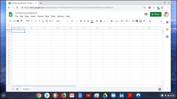
FIGURE 9-1: Google Sheets.
Surveying the Sheets menu area
The Sheets work area is broken into a couple of key areas: the menu area and the main document area, which is the actual spreadsheet. The menu area, by default, is composed of the Applications menu, Edit toolbar, and Formula bar, as shown in Figure 9-2.

FIGURE 9-2: The Sheets Application menu, Formula bar, and Edit toolbar.
The Applications menu in Google Sheets is located at the top of the menu area and is home to several application-specific controls and options, including
- File: File-specific options and controls for creating, saving, exporting, printing, and otherwise managing your document on the file level.
- Edit: Copy, paste, delete, and otherwise move and manipulate data.
- View: Modify your view by adding and removing toolbars or change the layout of the spreadsheet by adding or removing gridlines, freezing columns and rows, and more.
- Insert: Insert rows, columns, cells, worksheets, charts, images, and more.
- Format: Manipulate the appearance of your data, auto-format number data, align cell contents, and otherwise edit the appearance of your cells.
- Data: Sort and filter your data.
- Tools: Spell check, protect the sheet to ensure that data isn’t overwritten, or create a form to gather data.
- Add-ons: A gateway to adding features and functions to Google Sheets. This is a more advanced feature that I don’t discuss further in this book.
- Help: Get help with Sheets, search for menu options, and more.
The Edit toolbar, located directly under the Applications menu, contains several shortcuts to features contained in the Applications menu. The Edit toolbar makes the performance of routine tasks faster and easier. With the Edit toolbar, you can quickly perform these tasks on one or more cells in your worksheet:
- Print your worksheet, undo, or redo edits
- Format number data as currency or percentages
- Change fonts
- Change font size
- Bold, italicize, or strikethrough your text
- Color your text
- Fill a cell or cells with color
- Add, edit, or remove cell borders
- Merge multiple cells together into a single cell
- Edit the horizontal alignment of the contents of a cell
- Edit the vertical alignment of the contents of a cell.
- Allow text in a cell to wrap to multiple lines
- Add comments or charts, and perform common calculations
The Formula bar is located directly under the Edit toolbar. You use the Formula bar to insert data into cells and to type formulas for performing calculations.
Working with the spreadsheet area
The spreadsheet area of your Sheets workspace is located directly under the Formula bar. The spreadsheet is made up of a grid of columns and rows. The top of the columns is the column header, and the left side of the rows is the row header. Columns are referenced by letters (A, B, C, and so on), and rows are referenced by numbers (1, 2, 3, and so on). Permanent scroll bars are located at the right and bottom of your spreadsheet so that you can quickly scroll left and right, and up and down, through your spreadsheet.
At the bottom of the spreadsheet area, a tab labeled Sheet1 appears. The name of your current worksheet is Sheet1. You can, however, have multiple worksheets — represented by tabs — in one Sheets workbook.
Row numbers and column letters are imperative for precisely communicating locations within a spreadsheet. A cell’s coordinates are always communicated first with the column letter and then with the row number. For example, A8 means column A, row 8.
In Sheets, you refer to a range of cells in a single row or column by specifying the starting cell coordinates and the ending cell coordinates separated by a colon. For example:
A8:A20
This example references a range of cells starting in the A column at row 8 and ending at row 24. Figure 9-3 illustrates what this range looks like.
To reference a matrix of cells (meaning a range of cells, spanning multiple rows and columns), you specify the coordinates of the top-left corner and the bottom-right corner of the matrix separated by a colon. For example:
A8:C20
Figure 9-4 illustrates what this range looks like in the spreadsheet when selected.
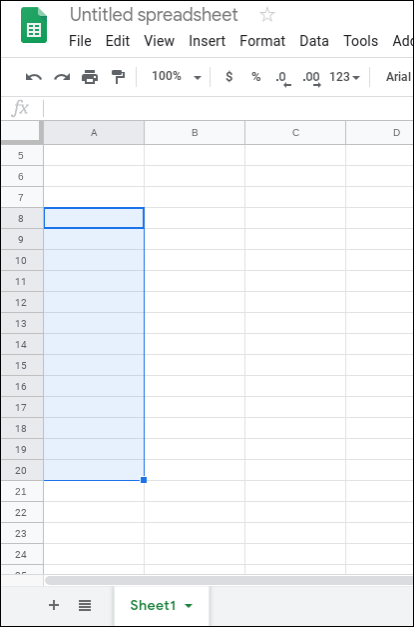
FIGURE 9-3: Cells A8 through A20.
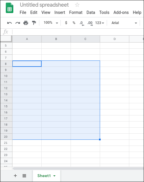
FIGURE 9-4: Cells A8 through C20.
Customizing your view
Before you dive into your first spreadsheet, you might find it helpful to change your view in Google Sheets.
If you prefer to hide the Applications menu, along with the Edit toolbar, you can do so by opening the View menu and choosing Full Screen. When you select Full Screen, the Applications menu and Edit toolbar vanish. (See Figure 9-5.)
 To exit Full Screen mode, simply press the Esc key.
If you prefer to have nothing but cells on your screen, you can remove the Applications menu, Edit toolbar, and Formula bar by following these steps:
- Click View in the Applications menu.
In the resulting View menu, choose Formula Bar.
The Formula bar vanishes.
Open the View menu again and choose Full Screen.
The Applications menu and Edit toolbar disappear, as shown in Figure 9-6.
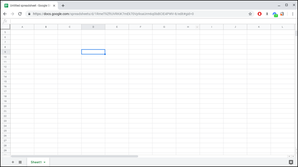
FIGURE 9-5: Google Sheets in Full Screen mode.
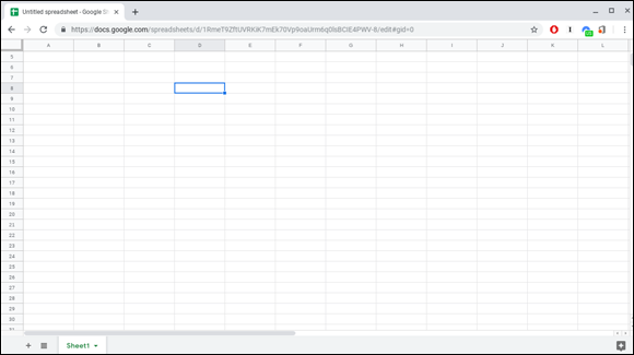
FIGURE 9-6: Google Sheets in Full Screen mode with no Formula bar.
In your spreadsheet, each cell is outlined with very thin gray lines called gridlines. Gridlines are not borders; they are imaginary boundaries, for reference only, and they won’t appear when you print your worksheet. If you would like to work without gridlines, you can hide them by opening the View menu and clicking Gridlines. Figure 9-7 shows a spreadsheet without gridlines.
To turn gridlines back on, just open the View menu and choose Gridlines.
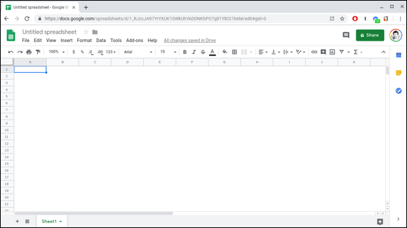
FIGURE 9-7: A Google Sheets spreadsheet without gridlines.
Working with Data
Spreadsheet software was developed to give you the ability to manipulate numeric data with great ease. That doesn’t mean, however, that the only data that can go into a spreadsheet is numeric data. You can type text and characters, or even add pictures and graphs.
Open a new Google Sheets spreadsheet. Cell A1 is highlighted with a blue border. This blue border indicates the active cell in your spreadsheet. Also notice that the A in the column heading is a darker gray than other columns, and that the 1 row heading on the left side is darker gray. If you click the left, right, up, and down arrows on your keyboard, notice that the blue cell outline moves, and the gray row and column indicators move as well. Clicking these arrows is the method for moving around in a worksheet. You can also move the cursor with your mouse or touchpad and click in a cell. On a touchscreen, simply touch the cell.
To enter data into a cell, make sure that the blue border is around a cell and begin typing. As you type, your entries appear in the highlighted cell, as well as in the Formula bar, as shown in Figure 9-8.
When you finish typing, press Enter to save what you’ve typed in the cell. Pressing Enter also moves the highlight bar to the next cell down. If the text you entered is larger than the cell, your text will hang over into adjacent cells until you resize the column width or row height. (I tell you about resizing cells in the section “Resizing columns and rows,” later in this chapter.)

FIGURE 9-8: Data entered appears in the selected cell and the Formula bar.
Moving around in a spreadsheet
As you enter more and more data into your spreadsheet, you may need to hop around to different cells to update your entries. You can move to different cells in a number of ways with Sheets. To start, take a look at the arrow keys on your keyboard.
Google Sheets can contain as many as 400,000 cells with a maximum of 256 columns. You don’t have to create the cells to be able to use them; you can simply navigate to them by using your directional arrows. Move one cell up, down, left, or right by pressing the corresponding directional arrow key once. If you want to quickly move several cells in any particular direction, press and hold the corresponding directional arrow.
You can also navigate your spreadsheet by using your touchpad or mouse. Click the desired cell once to move the cursor and then begin typing using your keyboard. If you need to get to a section of your sheet that is several rows down or columns over, you can quickly navigate there by following these steps:
Place two fingers on your touchpad and move them in the direction you desire.
If your touchpad is configured to traditionally scroll, swiping up scrolls up, and swiping down scrolls down. On the other hand, if your touchpad is configured to Australian scroll, swiping up scrolls down, and swiping down scrolls up. Using your touchpad with a two-finger swipe scrolls you to the general area of the cell or cells that you want to edit.
- Using one finger on your touchpad, move the pointer to the cell you desire.
Click your touchpad.
The desired cell is now active, enabling you to insert new text or change text that’s already there.
 To overwrite the cell contents, go to the cell, and simply start typing. To delete the cell contents, go to the cell, and press Backspace. To insert additional data in a cell that already contains data, follow these steps:
Click the desired cell once.
The selected cell is highlighted with a blue border.
Click the Formula bar.
A blinking cursor appears in the Formula bar, indicating that you can add, edit, or delete text using your keyboard.
- Add, edit, change, and remove text as you like; then press Enter.
You can also use a feature called Find and Replace to find a specific piece of data within your spreadsheet, as shown in Figure 9-9. To find data using the Find and Replace feature, follow these steps:
Open the Edit menu and choose Find and Replace.
The Find and Replace window appears. In this window, you can specify what you want to search for and what you want the search string replaced with, among other options.
You can move the window around on the screen in case it’s covering cells you’re working with.
Fill in the information you want to use for your search.
You can specify any of the following options:
- Find: The text or data you want to find.
- Replace: To replace the data for which you’re searching, simply enter new data here.
- Search: In this section, you can specify the scope of the search in a drop-down menu, including every sheet in your document, the current sheet, or a specific range of cells. You can also select boxes to match case or entire contents of a cell, or to search formulas and formula expressions.
- Match Case: Select this box to search for text exactly as you type it (regarding any use of upper- or lowercase, or any combination) in the Find box.
- Match Entire Cell Contents: The complete cell must match your search query.
- Search Using Regular Expressions: Search for a particular character pattern.
- Also Search within Formulas: Search formulas, in addition to the contents of cells.
Use the provided check boxes to fine-tune your search and reduce potentially inaccurate search results.- Click Find.
Sort through search results by clicking the Find button at the bottom-right of the Find and Replace pop-up window.
As you navigate through the search results in your document, Sheets changes the highlight color on the cell to indicate where you are in the spreadsheet.
When you successfully locate and replace the word or words in your spreadsheet, click the X in the top-right corner of the Find and Replace window to close that window.
The window disappears, but the text you searched for remains highlighted and ready to be deleted or otherwise edited.
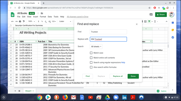
FIGURE 9-9: Find and Replace content in Google Sheets.
Copying and pasting data
As you enter data into your spreadsheet, you can avoid typing repetitive text by using the Copy and Paste functions. Copying and pasting can be done in a couple of ways — on the keyboard, with the touchpad, or a combination of both. To copy and paste a single cell, follow these steps:
Select the cell that you want to copy.
To copy and paste a range of cells, select the first cell in the range, hold the Shift key, and then select the last cell in the range.The selection area is highlighted in blue.
Open the Edit menu and choose Copy.
The selected cell’s contents are copied and stored in memory, also referred to as the Clipboard.
 The Clipboard can remember only one thing at a time. If you copy a selection of text and then copy another selection of text without pasting the first selection of text, Sheets forgets the first selection.
- Navigate to the cell where you want to paste the copied data.
Once again, open the Edit menu. This time, choose Paste.
The data copied to the Clipboard is now pasted into the selected cell.
When copying and pasting large areas of data, you can easily underestimate the amount of space needed for the paste and inadvertently overwrite meaningful data. However, you can undo any past action by clicking the Undo button in the Edit toolbar. The Undo button looks like an arrow in the shape of a half-circle pointing to the left. If you keep clicking Undo, your edits are undone, one at a time.
To paste the contents of one cell in a cell that’s several rows or columns away, you may find that the keyboard is too slow a means of navigating through your spreadsheet. Your touchpad offers a fast and convenient option to quickly copy and paste. To copy and paste a cell by using your touchpad, use the following steps:
- Using your touchpad, move your cursor to the cell you want to copy.
Tap the desired cell once to select it.
To select a range of cells, tap the first cell in the range and, without releasing your finger, move to the other end of the range you want to copy, and then release.Open the Edit menu and select Copy.
The selected cell is copied to the Clipboard.
Using your touchpad, scroll to the desired location, and tap the desired cell.
To paste a range of cells, select the cell you want to be the top-left corner of your pasted range.
Open the Edit menu and choose Paste.
The copied selection is pasted in.
To save time, you can use shortcut keys to copy and paste cells. Press Ctrl+C to copy a cell or cells, and press Ctrl+V to paste the copied cells. You can also quickly undo a paste (or many other actions) by pressing Ctrl+Z.
Alt-click your selection to reveal a menu of actions, including Copy and Paste. (See Figure 9-10.)
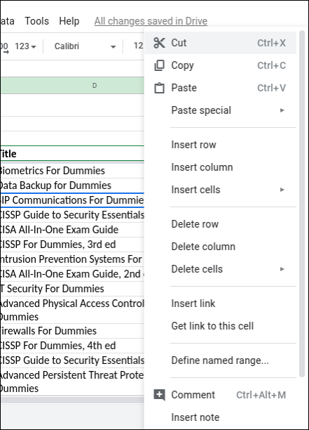
FIGURE 9-10: Actions that you can carry out on a cell or selection of cells in Google Sheets.
Moving data with Cut and Paste
When you want to replicate data, Copy and Paste is the mode of operation you should use. When you want to move data but not replicate it, however, use Cut. To move data in your sheet using the Cut and Paste method, follow these steps:
Using your touchpad, click to select the cell whose contents you want to move (or click and drag your cursor across all the cells whose contents you want to move) and then release.
The cell(s) are highlighted.
Alt-click the highlighted cell(s).
A pop-up menu appears, revealing several options.
Select Cut from the menu.
A dashed border surrounds your selection, indicating that the enclosed data has been cut.
- Using the touchpad, navigate to the location where you want to paste your data.
Alt-click the cell where you want to paste your data.
A pop-up menu appears.
Select Paste.
The data is moved accordingly.
You can paste data that you’ve cut as many times as you like. However, when you copy or cut a new selection of text, the previously cut text is replaced with the newly cut text.
Using Autofill to save time
The Autofill feature in Sheets makes it easy for you to copy and paste a particular pattern of data or to expand a series of data without having to manually enter the data or use the Copy and Paste feature repeatedly. To use Autofill to expand a series of data, follow these steps:
- In cell A1, type July 28.
- In cell A2, type July 29.
- In cell A3, type July 30.
Click cell A1 and select these cells by dragging your cursor down to cell A3.
Notice that a tiny blue square appears in the bottom-right corner of your selection, as pictured in Figure 9-11. This blue square is called the Autofill square, and it has magical power.
- Click the blue Autofill square and drag your selection down to Cell A10.
Release your click.
Sheets automatically fills your selection with the identified date sequence, as shown in Figure 9-12.
You can use Autofill to complete most sequences as long as you give Autofill enough information to guess what your sequence is. If Autofill can’t identify your sequence, it simply replicates your data as a pattern.

FIGURE 9-11: The Autofill square in Google Sheets.

FIGURE 9-12: Sheets completes the sequence of dates.
Formatting Data
Google Sheets gives you great control over the appearance of the content in your spreadsheet. You can change the formatting of a complete spreadsheet, rows, columns, or single cells. You can, in some instances, apply multiple style changes to the contents within a cell. For instance, you can apply different types of formatting, such as bold or italics, within one cell. On the other hand, you can’t mix font sizes within a single cell.
Google Sheets allows you to style your sheet in many different ways, including the following:
- Font formatting: Font means the style of typeface. With Sheets, you can change fonts, change the size or color of a font, or apply to a font new styles like bold, italics, underline, or strikethrough.
- Cell formatting: You can put borders around a cell or group of cells, or apply a background color. You can also auto-format numbers in a cell so that they take on a particular format. For example, you might want to auto-format currencies, percentages, dates, and times, to name a few.
- Alignment: You can change the horizontal alignment of the text within a cell to be left-, center- or right-aligned, or change the vertical alignment so that your text appears at the top, middle, or bottom of the cell. You can even style text so that it wraps to another line in your cell; this feature allows a cell with a lot of content to occupy multiple lines of text.
Working with fonts
With Sheets, you can change the font of any data contained in your spreadsheet. The options are potentially limitless, but for clarity, it’s better to limit the number of fonts that appear in one spreadsheet. Google Sheets comes preloaded with six fonts, and you can add more fonts if you need more. Your initial font options are
- Arial
- Comic Sans MS
- Courier New
- Georgia
- Impact
- Times New Roman
- Trebuchet MS
- Verdana
To change your font, follow these steps:
Using your touchpad, select the cells you want to change by clicking and dragging your cursor.
Sheets highlights the selected cells.
Open the Format menu; then open the Font submenu.
The Font submenu reveals available font choices.
The Font submenu is titled with the name of the font for the selected body of text. By default, all text appears in the Arial font.Select any one of the fonts listed.
The contents of the highlighted cells are changed to the selected font.
If the selected cells contain no data, the new font will apply to new text you add later.
Adding new fonts
The Google Sheets default list of fonts is a brief list of eight. Other spreadsheet programs such as Microsoft Excel or Apple Numbers have extensive lists of fonts by default. Google provides users with an initial list of the most globally popular fonts to keep things simple at first. You can, however, add fonts to your spreadsheets. To do so, follow these steps:
- Click the Font menu in the Edit toolbar.
Select More Fonts to add fonts.
The Font selection window, shown in Figure 9-13, gives you a robust list of new fonts from which to choose. Scroll down through the list to reveal more fonts.
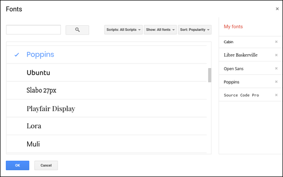
FIGURE 9-13: Adding new fonts to Google Sheets.
Select the desired fonts by clicking each one you want.
Each selected font is highlighted in blue and given a check mark.
Click OK to finish adding the fonts to your Font menu and exit.
When you are ready to change the font of your text, you will be able to choose from a list containing your original fonts, plus your newly selected fonts from the Font menu.
Adding fonts to Google Sheets makes these fonts available for Google Docs and Google Slides as well.
Removing fonts from the Font menu
The more fonts you add, the more fonts you will have to rifle through when trying to make a decision on changing the font of your text. Sometime in the future, you might decide that you have too many fonts and it’s time for some decluttering. To remove fonts from Sheets, take these steps:
- Open the Font menu in the Edit toolbar.
Select More Fonts.
The Font window appears. On the left of the window, a list of new fonts appears; on the right, a list of fonts currently in use by your Sheets account appears.
Scroll through the list of fonts on the right side of the window under My Fonts and locate the font or fonts you want to remove. Then, to remove a font, click the X located to the right of that font’s name.
The font disappears from the list of available fonts.
- Click OK.
Removing a font from your list of fonts does not affect your spreadsheets, even if they contain a font you removed from the menu. Further, after you use a font in your spreadsheet, you can change more text to use that font even if you removed it from your Font menu. (A removed font, however, will not be available in any new spreadsheets, or existing spreadsheets not containing the font.)
Styling your data
You can accentuate a font by applying various styles to the font itself, including
- Size: You can make your content bigger or smaller as you see fit.
- Bold: You can make content bold, which makes the text visibly thicker. Bold font is sometimes referred to as having a heavy weight.
- Italics: A slanted font is often referred to as italicized.
- Underline: Place a line under your content to indicate importance.
- Strikethrough: Place a line through the middle of your content. This is useful in communicating a change in your text or to illustrate a point.
- Color: Track changes, distinguish individual users in collaboration, or simply add style to your content by changing the color.
Changing font size
You can change the size of your content by following these steps:
Using your touchpad, select the cells you want to change by clicking and dragging your cursor.
The selected text is highlighted.
Open the Font Size menu in the Edit toolbar.
It’s the number found to the left of the Bold button in the Edit toolbar. When you click it, a menu appears, revealing several font sizes (in points) to choose from, as shown in Figure 9-14.
Select the desired font size.
Your selected data is now the chosen size.

FIGURE 9-14: Selecting font sizes in Google Sheets.
Applying bold, italics, underline, or strikethrough to your content
To apply formatting to a specific selection of cells, follow these steps:
Using your touchpad, select the cells you want to change by clicking and dragging your cursor.
The selected cells are highlighted.
Apply bold, italics, underline, or strikethrough, as needed.
You can use either of the following methods:
- To add bold, italics, or strikethrough: Click the appropriate button in the middle of the Edit toolbar — the B button for bold, the I button for italic, or the
Sbutton for strikethrough. (No button exists for the underline on the standard Edit toolbar.) - To add an underline: Open the Format menu in the application menu and select Underline.
Your selection changes appropriately.
- To add bold, italics, or strikethrough: Click the appropriate button in the middle of the Edit toolbar — the B button for bold, the I button for italic, or the
You can quickly apply styles to your data by using hotkeys. Just press Ctrl+B (for bold), Ctrl+I (italic), Ctrl+U (underline), or Alt+Shift+5 (strikethrough).
Coloring your content
Google Sheets gives you the ability to change the color of your data so that you can visually group your data, indicate important information, or just give your spreadsheet a little pizazz! To change the color of your data, follow these steps:
Using your touchpad, select the cells you want to change by clicking and dragging your cursor.
The selected cells are highlighted.
Open the Color menu in the Edit toolbar.
It's the A button found to the right of the S button.
A Color menu appears, revealing several color options, as shown in Figure 9-15.
Select your desired color.
The data in the selected cells now appears in the selected color.

FIGURE 9-15: Selecting colors for text in Google Sheets.
Changing alignment
Google Sheets gives you several options for changing the horizontal and vertical alignment of your data. Horizontal alignment options include
- Left
- Right
- Center
Vertical alignment options include
- Top
- Middle
- Bottom
To adjust the alignment of your data, follow these steps:
Using your touchpad, select the cells you want to realign by clicking and dragging your cursor.
The selected cells are highlighted.
In the Edit toolbar, find and click the appropriate Alignment button.
The Horizontal Alignment button is located a few buttons to the right of the text color button. The Vertical Alignment button is located to the right of the Horizontal Alignment button.
A menu with the alignment options appears.
Click the desired alignment.
The selected cells of data are realigned accordingly.
You can hover over the alignment buttons to see their function, as shown in Figure 9-16.
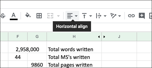
FIGURE 9-16: Hovering over alignment buttons reveal their purpose.
Wrapping text in a cell
By default, when you enter text into a cell, the text appears on a single line, so in order to show all the entered text, you may have to adjust the width of your cell. However, Sheets has a feature called wrap text that causes text to go to the next line after it reaches the maximum width of your cell. With this feature, you can set text to wrap in one cell or in every cell in a sheet. To activate wrap text, follow these steps:
Using your touchpad, select the desired cells by clicking and dragging your cursor.
The selected cells are highlighted.
- Open the Format menu.
Choose Wrap Text.
Text that extends beyond the boundaries of your cell walls will be wrapped to another line, as shown in Figure 9-17. In this figure, the text in cell B4 is too long for the cell, and it spills over the cells to the right. The text in cell B5 is set for wrap text, so all the text stays in the cell, which takes multiple lines.
Clearing formatting
Sometimes you just need to start over. The good news is that Sheets makes it incredibly easy to wipe out all formatting in a section of cells or your complete spreadsheet. To clear your formatting, follow these steps:

FIGURE 9-17: The wrap text feature in action.
Select the formatted cells you want to clear.
The selected cells are highlighted.
- Open the Format menu in the Applications menu.
Select Clear Formatting.
The selected data is reset to defaults: left-aligned, with all style elements — including color, underline, strikethrough, italics, bold, and so on — removed.
To clear the formatting of an entire document, press Ctrl+A instead of selecting cells. Pressing Ctrl+A selects the entire worksheet. (If your workbook has multiple worksheets or tabs, pressing Ctrl+A clears formatting only in the worksheet you are viewing.)
Customizing Your Spreadsheet
When you open Sheets for the first time (and when you click the + (plus sign) button to create a new spreadsheet), you're presented with a blank canvas of empty, uniform cells organized in a neat grid pattern. Sheets allows you to customize this grid of information so that it looks and works exactly how you like. In addition to all the text formatting discussed earlier, you can
- Change the height of rows and the width of individual (or all) columns
- Add and remove columns and rows
- Merge multiple cells together into one cell
- Hide rows and columns
- Add borders to individual cells and groups of cells
- Customize the background color of cells
Adding and deleting rows and columns
Adding rows or columns makes it easier to insert data into areas that are already populated with data. Instead of cutting and pasting data to make room, you can simply add an empty row or column.
The same goes for removing rows or columns. Deleting a column or row is a fast way to remove extraneous cells from your spreadsheet. When you get into formulas (see the section “Making Calculations with Formulas,” later in this chapter), you will also find that adding and deleting rows and columns keeps your formulas and formatting intact.
Adding a new row or column
You can add a new row or column by following these steps:
Using your touchpad, move your cursor to the row or column header of the row or column next to which you want to insert a new row or column and Alt-click the row or column header.
Column headers are indicated by a letter. Row headers are indicated by a number.
A menu appears, revealing several options. The menu for rows is shown in Figure 9-18.
Insert a new row by choosing Insert 1 Above or Insert 1 Below, or insert a new column by choosing Insert 1 Left or Insert 1 Right.
A new row or column is inserted accordingly.
You can see from the menu that you can do other things with a row or column, including:
- Delete a row or column
- Clear a row or column
- Hide a row or column
- Resize a row or column (meaning, its width or height)
- Group all cells in a row or column into a single cell
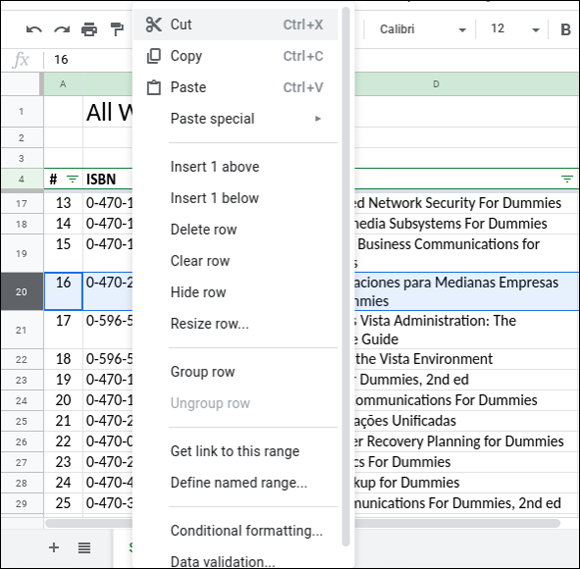
FIGURE 9-18: The Alt-click menu for rows in Google Sheets.
Don’t worry about making your spreadsheet too big. Size is never a problem. The largest spreadsheet you can make with Sheets can have up to 400,000 cells and as many as 256 columns.
Deleting a row or column
You can delete a row or column by following these steps:
- Using your touchpad, move your cursor to the header of the row or column you want to delete.
Alt-click the row number or column letter.
A menu appears, revealing several options.
Click Delete Row or Delete Column.
The row or column is deleted. The remaining rows or columns move together to fill the gap.
Resizing columns and rows
The row and column sizes in Google Sheets are set by default to an arbitrary size. You can build a perfectly functional spreadsheet and never resize any columns or rows. However, resizing is a great way to ensure that your data is viewable and useful. If a string of text is too big for the current column width or row height, Sheets lets you quickly change the width or height to accommodate your needs. Also, if your columns are too wide or your rows too high, which may result in your having to scroll back and forth (or up and down) to view all your content, you can make some columns narrower (or rows shorter), which makes room for more content to appear on your screen.
To resize your column or row, follow these steps:
Using your touchpad, move your pointer to the column or row header you want to resize.
Make sure that your pointer is over the line on the right side of the column or bottom side of the row that you would like to resize.
Your pointer turns into a set of arrows.
- Click and drag to change the size of the column or row.
- When you are satisfied with the new size, release your click.
You can also change the size of multiple rows or columns at the same time. To do so, the columns or rows must be sequential. For example, you can resize columns 1, 2, and 3 at the same time, but you can’t resize columns 1, 2, and 5 at the same time. To resize multiple columns or rows, follow these steps:
Using your touchpad, click the header for the first column or row in the series you want to resize.
The selected row or column is highlighted.
Shift-click the header for the last of the columns or rows in the series you want to resize.
Every row or column in the series is selected.
Relocate your pointer so that it rests over the line dividing two rows or columns in your selection.
The pointer turns into a set of arrows.
- Click and drag the column or row to resize.
When you’re satisfied, release your click.
Each row or column in the series is resized.
Hiding columns and rows
Hiding rows and columns is handy when you’re presenting a spreadsheet and want to hide a row or column of notes, or when some of your data is necessary for calculations but not relevant enough to be shown. Hiding is a great way to keep data in its place but out of sight. To hide a row or column, follow these steps:
- Using your touchpad, move your pointer over the header of the row or column you want to hide.
Alt-click the row or column header.
A menu appears, revealing several options.
Select Hide Column or Hide Row, whichever is appropriate.
The associated row or column vanishes, leaving only a set of arrows over the column or row dividing line.
To restore your hidden column or row, click these arrows.
Merging cells
Sometimes you will want or even need to have a heading over several columns or rows. To do this, you need to merge multiple cells together so that they form a single cell spanning multiple columns or rows. To merge cells together, follow these steps:
Shift-click the contiguous cells you want to merge.
The selected cells become highlighted.
Click the Merge Cells button in the Edit toolbar, located nine buttons from the right.
The highlighted cells merge.
Any data in merged cells may be lost. Be sure to have a copy of the cell’s contents prior to merging.To unmerge the cells, select the newly merged cell and click the Merge Cells button again.
The cells that you merged are restored to being individual cells. If you placed content in the merged cell, that content will appear in the first row or column of the previously merged set.
Formatting numbers
People use spreadsheets primarily to organize and calculate numeric data. With Google Sheets, you can auto-format your cells to accommodate several numeric data types, including
- Currency
- Percentages
- Decimals
- Financial notation
- Scientific notation
- Dates
- Times
Formatting cells for these numeric types can be done by following these steps:
- Using your touchpad, select the cell or cells you want to format.
- Open the Format menu.
Move your pointer over Number in the menu.
A submenu appears, revealing several formatting options.
Select the desired formatting style, as shown in Figure 9-19.
The selected cells now auto-format numeric entries to match the selected style.
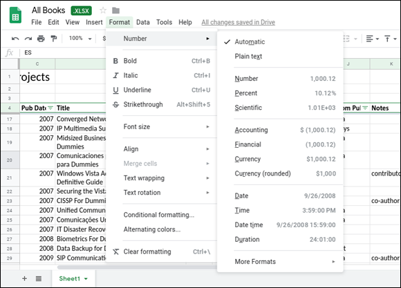
FIGURE 9-19: Applying auto-formatting to selected cells in Google Sheets.
Grouping cells with colors and borders
When working with spreadsheets containing large amounts of data, the numbers and letters can begin to blend together. You can distinguish groups of cells with borders or colors to make navigating your spreadsheet easier. Borders and cell shading can also add a nice touch of style to your spreadsheets. You can add borders to your spreadsheet by following these steps:
Using your touchpad, select the cells you want to style by clicking and dragging your cursor.
The selected cells are highlighted.
Click the Border button in the Edit toolbar.
The Border button, which looks like a little square with four squares inside, is a few buttons to the right of the Bold, Italic, and Strikethrough formatting buttons.
A menu appears, giving you several options.
To simply place a border around your cells, locate the image that shows a border outline and click it.
The images in the Border menu, as shown in Figure 9-20, illustrate precisely where the border will go if selected. You can also change the border style to dotted or dashed by selecting the Line option in the Border Style menu, or change the color of your border by using the Border Color option.
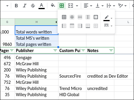
FIGURE 9-20: Adding a border to cells in Google Sheets.
You can also create visual separation in your spreadsheet by incorporating color into your cells. To apply a color background to a cell or group of cells, follow these steps:
Using your touchpad, select the cells you want to color by clicking and dragging your cursor.
The selected cells are highlighted.
Click the Background Color button in the Edit toolbar.
This button is located just to the right of the Bold, Italic, and Strikethrough buttons and looks like a paint can being poured out. When you hover over the button, the words Fill Color appear.
A menu appears, giving you several options.
Select a color from the menu.
The background of the selected cells is changed to the chosen color.
Making Calculations with Formulas
Google Sheets is a powerful spreadsheet tool. With Sheets, you can perform analysis on text and numeric values alike, and incorporate financial, mathematical, and statistical analysis. The following sections serve as an intro to Sheets’ basic functions and formulas.
Adding basic mathematical formulas
Sheets can perform mathematical calculations for you. All you have to do is tell Sheets that you want it to perform a calculation on the information you enter in the cell. To do this, you must start your equation with an equals sign (=). Make sheets do basic addition by following these steps:
- With Sheets open, select a cell.
- Type the following string of characters precisely:
=50+50 Press Enter.
Sheets solves the equation and displays the answer, 100.
Although the cell itself displays 100, if you look on the Formula bar, you see the formula that still reads what you typed in: =50+50.
You can use several mathematical operators to perform calculations with Sheets. They include
- Addition: +
- Subtraction: –
- Division: /
- Multiplication: *
Sheets interprets the order of operations according to simple rules: It performs calculations within parentheses first, followed by multiplication or division (from left to right), and finally, addition or subtraction (from left to right).
To ensure that Sheets always follows the mathematical order of operations you intended, use parentheses to group operations together. For example, in a cell, enter the following equation:
=((5+5)*8)/2
You get the answer 40. When more than one set of parentheses exists, Sheets performs the instructions within the innermost set first and then works its way outward. Without parentheses, the equation becomes
=5+5*8/2
This returns the answer 25. Use parentheses to ensure that your operations are performed in the order you intended.
Building formulas can become complex very quickly. To edit a formula, select the cell that contains the formula and then click in the Formula bar at the top of your Sheets window to edit the formula. Typing in the cell itself overwrites the contents, leaving you to start again!
Adding formulas to calculate values in cells
Google Sheets was designed for use beyond just standard calculator functions. You can also use Sheets to perform calculations using data in multiple cells within your spreadsheet. Instead of entering numbers into your equations, you can enter cell coordinates. To see how this works, you first have to have numbers in some cells, so this example walks you through adding some data and then entering the formula for Sheets to calculate:
- With Sheets open, enter the number 25 into cell A2.
- Enter the number 50 into cell A3.
- Enter the number 75 into cell A4.
- In cell B5, enter the following equation:
=A2+A3+A4 Press Enter.
Sheets adds cells A2, A3, and A4 together and then displays the answer — 150 — in cell B5.
Next, try changing the data in any of the cells A2, A3, or A4, and see how the value in cell B5 changes immediately.
Don’t forget to put the equals sign (=) before a formula, otherwise the contents of the cell will contain the characters in the formula, instead of the result that Sheets would get by performing the calculation.
You can also use Google Sheets to perform a calculation using values in cells along with other values in the formula. Try it yourself with these steps:
- With Sheets open, enter the number 25 into cell A2.
- Enter the number 50 into cell A3.
- Enter the number 75 into cell A4.
- In cell A5, enter the following equation:
=(A2+A3+A4)*10 Press Enter.
Sheets adds cells A2, A3, and A4 together and then multiplies the total by 10. The resulting answer is 1500, which it displays in cell A5, as shown in Figure 9-21.
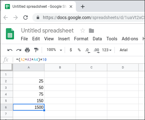
FIGURE 9-21: Using formulas in Google Sheets to add the values of cells together.
Working with spreadsheet functions
Sheets has an extensive library of functions that perform a vast array of computations. However, the most widely used functions in Sheets are
- SUM: Adds all the numbers in a range of cells.
- AVERAGE: Outputs the average of the values in a specific set of cells or in a range.
- COUNT: Count how many numbers are in a list of cells. You can specify cells or enter a range.
- MAX: Outputs the largest number in a specific set of cells or a range.
- MIN: Outputs the smallest number in a specific set of cells or a range.
Functions simplify the process of writing complex formulas and reduce the amount of typing needed to get the desired result. To try using the SUM function, follow these steps:
- With Sheets open, enter the number 25 into cell A2.
- Enter the number 50 into cell A3.
- Enter the number 75 into cell A4.
- In cell A6, enter the following equation:
=SUM(A2:A4) Press Enter.
The formula tells Sheets that you want to add the values in cells A2 through A4. The output value is 150, which Sheets displays in cell A6.
- To use parentheses to set the order in which functions are used in the equation, in cell A6, enter the following equation:
=(SUM(A2:A4)*10) Press Enter.
Sheets first calculates the sum of the values in cells A2 through A4 and then multiplies the total by 10, displaying 1500 in cell A6. This is shown in Figure 9-22. Note the content in the Formula bar and how it differs from the Formula bar in Figure 9-21.
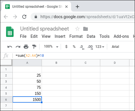
FIGURE 9-22: Using functions to add the contents of cells together.
Saving Documents
As you work in Google Sheets, Google will save almost every change in real-time to your Google Drive account (remember that Google Drive is your cloud-based storage that allows you to safely store your files and access them from any device with an Internet connection). Every file you create with Google Sheets is saved to your Drive folder so that you can access it at home, on the road, at work, or anywhere else you might need to, and from any device you happen to be using at the time. As is the case with Docs, Sheets has no manual Save feature.
Naming your document
When you open a new spreadsheet with Sheets, the default name for the spreadsheet is Untitled Spreadsheet. You don’t, however, want to leave your spreadsheet untitled. Drive doesn’t have a problem with storing multiple files with the same name, but it’s best if you name your spreadsheet immediately so that you save yourself a little confusion. To name your spreadsheet, follow these steps:
Open a new spreadsheet.
The easiest way to open a new spreadsheet is by launching Sheets from the Launcher.
A Chrome web browser opens and loads Sheets.
Click the “+” to start a new worksheet.
After Sheets is open, the name of your new document, Untitled Spreadsheet, appears in the top-left corner, as shown in Figure 9-23.
Click Untitled Spreadsheet in the top-left corner of your spreadsheet.
The cursor is positioned preceding the words Untitled Spreadsheet.
Type the new name for your spreadsheet and press Enter.
The name Untitled Spreadsheet is now replaced with your new name.
The next time you look at Google Drive, you’ll see the new filename, which is your renamed spreadsheet. As you continue to make edits, the spreadsheet document will be updated and saved in real time.
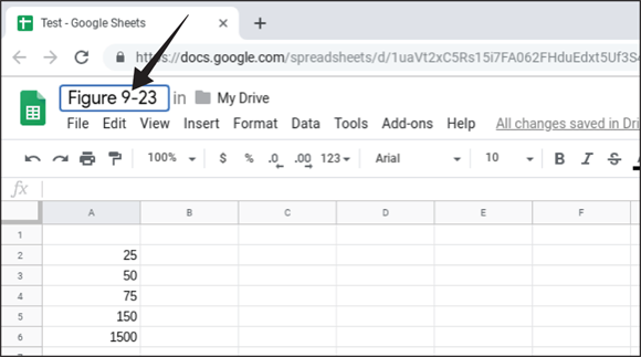
FIGURE 9-23: You can change the spreadsheet’s name.
Exporting documents
From time to time, you may need to export your spreadsheets to formats that others may be comfortable with. Sheets allows you to export spreadsheets to a few standard formats, including
- Microsoft Excel (
.xlsx) - OpenDocument (
.ods) - PDF (
.pdf) - Comma-separated values (
.csv) - Tab-separated values (
.tsv) - Web page (
.html)
Exporting documents to different file types may change the formatting within your document. For example, exporting to the CSV and TSV formats strips out all formatting, such as borders, fonts, and colors. Before sending along your spreadsheets after an export, you should review them to ensure that everything is as it should be!
You can export your documents by following these steps:
Click File and hover your cursor over Download As.
A submenu appears, revealing the file types that are available for export.
Select the desired file type.
You see a preview of your exported spreadsheet.
Click the Export button in the upper right of the Sheets window.
Google Sheets now asks you to specify the name of the file to create, as well as the location. By default, your file will be located in the Downloads folder. You can, however, click a different folder on the left side of the Save File As window, including Google Drive or even a folder within Google Drive.
Click the folder you want to save the file in, click the filename, and then click Save.
Your spreadsheet is exported in the desired file type to the location you specified. (Take a look at Figure 9-24.)
- To view the downloaded file, open the Files app, go to the folder you specified in Step 4, and look for the file.
When you export a spreadsheet, there are several options in the Export window, including whether you want to export just the tab displayed or all tabs, page orientation (portrait or landscape), formatting, margins, and more. Try these to see how your exported spreadsheet appears. (You can always delete these files later using the Files app.)
Exporting a spreadsheet doesn’t change the original spreadsheet; instead, it makes a copy of it in the specified format. The original Google Sheets file is still there, and you can continue to edit it as much as you like.
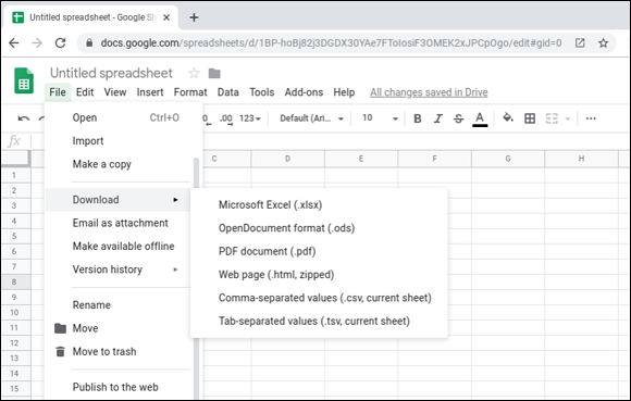
FIGURE 9-24: Exporting a spreadsheet to a folder in Google Drive.
Collaboration with Sheets
By default, Google Sheets and Google Drive make your files inaccessible to everyone other than you. You can, however, change the visibility settings on your files and invite specific people, or even the entire world, to comment, view, or edit your document! To share your Spreadsheet with specific people, follow these steps:
Click the blue Share button in the top-right corner of your Sheets window.
A window appears, giving you several options for sharing your spreadsheet.
Enter the email address of each person with whom you want to share your file in the Invite People field at the bottom of the window.
Be sure to separate the addresses with commas.
If the email address is in your address book, Sheets tries to autofill the information.
To set the permissions of the collaborators, first click the link directly to the right of the Invite People field.
A menu with three options appears:
- Can Edit: Allows users to edit the spreadsheet, comment, view, and change permissions
- Can Comment: Allows users to view and comment on the spreadsheet but not to change any content or security settings
- Can View: Allows users only to view the spreadsheet; they cannot make any changes
- Select the appropriate permission setting from the menu.
- Type any comments in the Comments box if you want to send any instructions to the people you share your spreadsheet with.
Click Send.
Your document is made available to the users immediately, as shown in Figure 9-25.
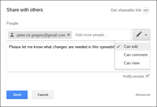
FIGURE 9-25: Sharing a spreadsheet with other people.
The users who are invited to view, edit, or comment on your spreadsheet have to log in to Google Docs using the email addresses with which you shared the spreadsheet. If a user doesn’t have a Google Account under the email address you used, you have to invite her with the address she uses for her Google Account. She also has the option to create a Google Account using the same email address.
Tracking Versions of Your Spreadsheet
Keeping track of revisions is very important when creating documents with multiple collaborators. Fortunately, Google Sheets handles version control masterfully. As you and your collaborators make changes to your spreadsheets, Sheets stamps those changes with the time and date so that you can view previous versions of your spreadsheet and even revert to an earlier version if you need to.
Version tracking is a default feature of Google Sheets, so you don’t need to do anything to take advantage of it. To view your version history, follow these steps:
Open the File menu, hover over Version History, and tap See Version History.
A Version History box appears in the right portion of your screen. The box contains the various versions of your spreadsheet in order from the most recent to the oldest. If you made multiple changes on any given day, a tiny black arrow appears to the left of the date; click the arrow to see the details for that date. The names of the people who saved the spreadsheet are also shown. (If you are not sharing your spreadsheet, it will always be your name.) See Figure 9-26.
Click a version date in the Version History box.
A preview of the version you chose appears in the main document area. Changes that occurred between versions appear in green.
To change versions, click Restore This Version.
Google Sheets will ask you to name this version.
The restored version becomes the current version, and the previous version of the application is saved in the Version History, so you can revert back to it if needed.
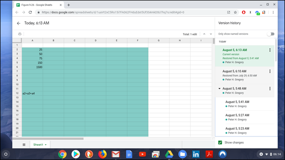
FIGURE 9-26: Viewing versions of a spreadsheet in Google Sheets.
Using Sheets Offline
Google Sheets is a web-based spreadsheet tool, which means that you must have an Internet connection to access all its features. However, an offline version of Sheets is available in the event that you find yourself without a connection to the Internet.
While offline, you can’t access some of the features available to Sheets users who are connected to the Internet (such as downloading new fonts). You can, however, create spreadsheets and save them. Later, when you connect to the Internet, Drive uploads the saved spreadsheets and enables all Internet-only features.
To use Google Sheets offline, you must first enable Google Drive for offline use. Follow these steps to make sure that you’re set up for offline use:
Open the Launcher and click the Google Drive icon.
A Chrome web browser appears and takes you to your drive.
- On the right side of the screen, click the Settings icon (it looks like a gear).
In the resulting menu, click Settings.
The Settings window appears.
- In the Offline section, select the check box that reads, Create, Open and Edit your recent Google Docs, Sheets, and Slides on This Device While Offline to sync your work for offline use.
Click Done.
Your Sheets files are now synced and available for offline editing. You can test whether you have properly enabled offline access by turning off your Wi-Fi.
Open the Settings panel in the bottom-right of your screen and click the blue Wi-Fi icon.
The Wi-Fi icon turns from blue to gray, indicating that your Chromebook is no longer connected to the Internet.
With your Wi-Fi turned off, switch back to Google Drive and open one of your synced spreadsheets.
If your spreadsheet opens and you are able to edit it, you know that you have successfully engaged offline use and synced your documents.