
Data transformations
Abstracts
There are many transformations that can make real-world datasets more amenable to the learning algorithms discussed in the rest of the book. We first consider methods for attribute selection, which remove attributes that are not useful for the task at hand. Then we look at discretization methods: algorithms for turning numeric attributes into discrete ones. Next we discuss several techniques for projecting data into a space that is more suitable for learning: well-known methods for dimensionality reduction, including unsupervised approaches such as principal component analysis, independent component analysis, and random projections, as well as supervised approaches such as partial least squares regression and linear discriminant analysis. We consider how to turn textual data into numeric attribute vectors so that standard learning techniques can be applied, and present simple methods for approaching time series data. The last four sections deal with data sampling, data cleansing, generic approaches for multiclass classification, and calibration of class probabilities, respectively. Sampling is nontrivial when the data arrives as a stream, and we discuss the “reservoir” method for taking an unbiased sample in this case. Data cleansing can be performed by iteratively applying standard supervised learning algorithms to remove outliers, but there are also dedicated techniques for anomaly detection and so-called “one-class learning” that are applicable. For dealing with multiclass classification problems, we consider several ways of decomposing them into a set of two-class problems, e.g., by applying error-correcting output codes. Finally, we describe how to calibrate class probability estimates to improve their accuracy.
Keywords
Data transformations; attribute selection; dimensionality reduction; vector space model; data sampling; data cleansing; multiclass classification; class probability calibration
In the previous chapters we examined a large array of machine learning methods: decision trees, classification and association rules, linear models, instance-based schemes, numeric prediction techniques, and clustering algorithms. All are sound, robust techniques that are eminently applicable to practical data mining problems.
But successful data mining involves far more than selecting a learning algorithm and running it over your data. For one thing, many learning schemes have various parameters, and suitable values must be chosen for these. In most cases, results can be improved markedly by suitable choice of parameter values, and the appropriate choice depends on the data at hand. For example, decision trees can be pruned or unpruned, and in the former case a pruning parameter may have to be chosen. In the k-nearest-neighbor method of instance-based learning, a value for k will have to be chosen. More generally, the learning scheme itself will have to be chosen from the range of schemes that are available. In all cases, the right choices depend on the data itself.
It is tempting to try out several learning schemes, and several parameter values, on your data, and see which works best. But be careful! The best choice is not necessarily the one that performs best on the training data. We have repeatedly cautioned about the problem of overfitting, where a learned model is too closely tied to the particular training data from which it was built. It is incorrect to assume that performance on the training data faithfully represents the level of performance that can be expected on the fresh data to which the learned model will be applied in practice.
Fortunately, we have already encountered the solution to this problem in Chapter 5, Credibility: evaluating what's been learned. There are two good methods for estimating the expected true performance of a learning scheme: the use of a large dataset that is quite separate from the training data, in the case of plentiful data, and cross-validation (Section 5.3), if data is scarce. In the latter case, a single 10-fold cross-validation is typically used in practice, although to obtain a more reliable estimate the entire procedure should be repeated 10 times. Once suitable parameters have been chosen for the learning scheme, use the whole training set—all the available training instances—to produce the final learned model that is to be applied to fresh data.
Note that the performance obtained with the chosen parameter value during the tuning process is not a reliable estimate of the final model’s performance, because the final model potentially overfits the data that was used for tuning. We discussed this in Section 5.5. To ascertain how well it will perform, you need yet another large dataset that is quite separate from any data used during learning and tuning. The same is true for cross-validation: you need an “inner” cross-validation for parameter tuning and an “outer” cross-validation for error estimation. With 10-fold cross-validation, this involves running the learning scheme 100 times for each parameter setting being considered. To summarize: When assessing the performance of a learning scheme, any parameter tuning that goes on should be treated as though it were an integral part of the training process.
There are other important processes that can materially improve success when applying machine learning techniques to practical data mining problems, and these are the subject of this chapter. They constitute a kind of data engineering: engineering the input data into a form suitable for the learning scheme chosen and engineering the output to make it more effective. You can look on them as a bag of tricks that you can apply to practical machine learning problems to enhance the chance of success. Sometimes they work; other times they do not—and at the present state of the art, it is hard to say in advance whether they will or not. In an area such as this where trial and error is the most reliable guide, it is particularly important to be resourceful and have an understanding of what the tricks are.
In this chapter we examine six different ways in which the input can be massaged to make it more amenable for learning methods: attribute selection, attribute discretization, data projections, sampling, data cleansing, and converting multiclass problems to two-class ones. Consider the first, attribute selection. In many practical situations there are far too many attributes for learning schemes to handle, and some of them—perhaps the overwhelming majority—are clearly irrelevant or redundant. Consequently, the data must be preprocessed to select a subset of the attributes to use in learning. Of course, many learning schemes themselves try to select attributes appropriately and ignore irrelevant or redundant ones, but in practice their performance can frequently be improved by preselection. For example, experiments show that adding useless attributes causes the performance of learning schemes such as decision trees and rules, linear regression, and instance-based learners to deteriorate.
Discretization of numeric attributes is absolutely essential if the task involves numeric attributes but the chosen learning scheme can only handle categorical ones. Even schemes that can handle numeric attributes often produce better results, or work faster, if the attributes are prediscretized. The converse situation, in which categorical attributes must be represented numerically, also occurs (although less often); and we describe techniques for this case, too.
Data projection covers a variety of techniques. One transformation, which we have encountered before when looking at relational data in Chapter 2, Input: concepts, instances, attributes, and support vector machines in Chapter 7, Extending instance-based and linear models, is to add new, synthetic attributes whose purpose is to present existing information in a form that is suitable for the machine learning scheme to pick up on. More general techniques that do not depend so intimately on the semantics of the particular machine learning problem at hand include principal component analysis and random projections. We also cover discriminant analysis for classification and partial least squares regression as a data projection technique for regression problems.
Sampling the input is an important step in many practical data mining applications, and is often the only way in which really large-scale problems can be handled. Although it is fairly simple, we include a brief section on techniques of sampling, including a way of incrementally producing a random sample of given size when the total size of the dataset is not known in advance.
Unclean data plagues data mining. We emphasized in Chapter 2, Input: concepts, instances, attributes, the necessity of getting to know your data: understanding the meaning of all the different attributes, the conventions used in coding them, the significance of missing values and duplicate data, measurement noise, typographical errors, and the presence of systematic errors—even deliberate ones. Various simple visualizations often help with this task. There are also automatic methods of cleansing data, of detecting outliers, and of spotting anomalies, which we describe—including a class of techniques referred to as “one-class learning” in which only a single class of instances is available at training time.
Finally, we examine techniques for refining the output of learning schemes that estimate class probabilities by recalibrating the estimates that they make. This is primarily of importance when accurate probabilities are required, as in cost-sensitive classification, although it can also improve classification performance.
8.1 Attribute Selection
Most machine learning algorithms are designed to learn which are the most appropriate attributes to use for making their decisions. For example, decision tree methods choose the most promising attribute to split on at each point and should—in theory—never select irrelevant or unhelpful attributes. Having more features should surely—in theory—result in more discriminating power, never less. “What’s the difference between theory and practice?” an old question asks. “There is no difference between theory and practice,” the answer goes, “—in theory. But in practice, there is.” Here there is too: in practice, adding irrelevant or distracting attributes to a dataset often confuses machine learning systems.
Experiments with a decision tree learner (C4.5) have shown that adding to standard datasets a random binary attribute generated by tossing an unbiased coin impacts classification performance, causing it to deteriorate (typically by 5–10% in the situations tested). This happens because at some point in the trees that are learned, the irrelevant attribute is invariably chosen to branch on, causing random errors when test data is processed. How can this be, when decision tree learners are cleverly designed to choose the best attribute for splitting at each node? The reason is subtle. As you proceed further down the tree, less and less data is available to help make the selection decision. At some point, with little data, the random attribute will look good just by chance. Because the number of nodes at each level increases exponentially with depth, the chance of the rogue attribute looking good somewhere along the frontier multiplies up as the tree deepens. The real problem is that you inevitably reach depths at which only a small amount of data is available for attribute selection. This is known as the fragmentation problem. If the dataset were bigger it wouldn’t necessarily help—you’d probably just go deeper.
Divide-and-conquer tree learners and separate-and-conquer rule learners both suffer from this effect because they inexorably reduce the amount of data on which they base judgments. Instance-based learners are very susceptible to irrelevant attributes because they always work in local neighborhoods, taking just a few training instances into account for each decision. Indeed, it has been shown that the number of training instances needed to produce a predetermined level of performance for instance-based learning increases exponentially with the number of irrelevant attributes present. Naïve Bayes, by contrast, does not fragment the instance space and robustly ignores irrelevant attributes. It assumes by design that all attributes are independent of one another, an assumption that is just right for random “distracter” attributes. But through this very same assumption, Naïve Bayes pays a heavy price in other ways because its operation is damaged by adding redundant attributes.
The fact that irrelevant distracters degrade the performance of decision tree and rule learners is, at first, surprising. Even more surprising is that relevant attributes can also be harmful. For example, suppose that in a two-class dataset a new attribute were added, which had the same value as the class to be predicted most of the time (65%) and the opposite value the rest of the time, randomly distributed among the instances. Experiments with standard datasets have shown that this can cause classification accuracy to deteriorate (by 1–5% in the situations tested). The problem is that the new attribute is (naturally) chosen for splitting high up in the tree. This has the effect of fragmenting the set of instances available at the nodes below so that other choices are based on sparser data.
Because of the negative effect of irrelevant attributes on most machine learning schemes, it is common to precede learning with an attribute selection stage that strives to eliminate all but the most relevant attributes. The best way to select relevant attributes is manually, based on a deep understanding of the learning problem and what the attributes actually mean. However, automatic methods can also be useful. Reducing the dimensionality of the data by deleting unsuitable attributes improves the performance of learning algorithms. It also speeds them up, although this may be outweighed by the computation involved in attribute selection. More importantly, dimensionality reduction yields a more compact, more easily interpretable representation of the target concept, focusing the user’s attention on the most relevant variables.
Scheme-Independent Selection
When selecting a good attribute subset, there are two fundamentally different approaches. One is to make an independent assessment based on general characteristics of the data; the other is to evaluate the subset using the machine learning algorithm that will ultimately be employed for learning. The first is called the filter method, because the attribute set is filtered to produce the most promising subset before learning commences. The second is the wrapper method, because the learning algorithm is wrapped into the selection procedure. Making an independent assessment of an attribute subset would be easy if there were a good way of determining when an attribute was relevant to choosing the class. However, there is no universally accepted measure of “relevance,” although several different ones have been proposed.
One simple scheme-independent method of attribute selection is to use just enough attributes to divide up the instance space in a way that separates all the training instances. For example, if just one or two attributes are used, there will generally be several instances that have the same combination of attribute values. At the other extreme, the full set of attributes will likely distinguish the instances uniquely so that no two instances have the same values for all attributes. (This will not necessarily be the case, however; datasets sometimes contain instances with the same attribute values but different classes.) It makes intuitive sense to select the smallest attribute subset that serves to distinguish all instances uniquely. This can easily be found using exhaustive search, although at considerable computational expense. Unfortunately, this strong bias toward consistency of the attribute set on the training data is statistically unwarranted and can lead to overfitting—the algorithm may go to unnecessary lengths to repair an inconsistency that was in fact merely caused by noise.
Machine learning algorithms can be used for attribute selection. For instance, you might first apply a decision tree algorithm to the full dataset, and then select only those attributes that are actually used in the tree. While this selection would have no effect at all if the second stage merely built another tree, it will have an effect on a different learning algorithm. For example, the nearest-neighbor algorithm is notoriously susceptible to irrelevant attributes, and its performance can be improved by using a decision tree builder as a filter for attribute selection first. The resulting nearest-neighbor scheme can also perform better than the decision tree algorithm used for filtering. As another example, the simple 1R scheme described in Chapter 4, Algorithms: the basic methods, has been used to select the attributes for a decision tree learner by evaluating the effect of branching on different attributes (although an error-based method such as 1R may not be the optimal choice for ranking attributes, as we will see later when covering the related problem of supervised discretization). Often the decision tree performs just as well when only the two or three top attributes are used for its construction—and it is much easier to understand.
Another possibility is to use an algorithm that builds a linear model—e.g., a linear support vector machine—and ranks the attributes based on the size of the coefficients. A more sophisticated variant applies the learning algorithm repeatedly. It builds a model, ranks the attributes based on the coefficients, removes the lowest-ranked one, and repeats the process until all attributes have been removed. This method of recursive feature elimination has been found to yield better results on certain datasets (e.g., when identifying important genes for cancer classification) than simply ranking attributes based on a single model. With both methods it is important to ensure that the attributes are measured on the same scale; otherwise, the coefficients are not comparable. Note that these techniques just produce a ranking; another method must be used to determine the appropriate number of attributes to use.
Attributes can be selected using instance-based learning methods too. You could sample instances randomly from the training set and check neighboring records of the same and different classes—“near hits” and “near misses.” If a near hit has a different value for a certain attribute, that attribute appears to be irrelevant and its weight should be decreased. On the other hand, if a near miss has a different value, the attribute appears to be relevant and its weight should be increased. Of course, this is the standard kind of procedure used for attribute weighting for instance-based learning, described in Section 7.1. After repeating this operation many times, selection takes place: only attributes with positive weights are chosen. As in the standard incremental formulation of instance-based learning, different results will be obtained each time the process is repeated, because of the different ordering of examples. This can be avoided by using all training instances and taking into account all near hits and near misses of each.
A more serious disadvantage is that the method will not detect an attribute that is redundant because it is correlated with another attribute. In the extreme case, two identical attributes would be treated in the same way, either both selected or both rejected. A modification has been suggested that appears to go some way towards addressing this issue by taking the current attribute weights into account when computing the nearest hits and misses.
Another way of eliminating redundant attributes as well as irrelevant ones is to select a subset of attributes that individually correlate well with the class but have little intercorrelation. The correlation between two nominal attributes A and B can be measured using the symmetric uncertainty:
where H is the entropy function described in Section 4.3. The entropies are based on the probability associated with each attribute value; H(A,B), the joint entropy of A and B, is calculated from the joint probabilities of all combinations of values of A and B. The symmetric uncertainty always lies between 0 and 1. Correlation-based feature selection determines the goodness of a set of attributes using

where C is the class attribute and the indices i and j range over all attributes in the set. If all m attributes in the subset correlate perfectly with the class and with one another, the numerator becomes m and the denominator ![]() , which is also m. Hence the measure is 1, which turns out to be the maximum value it can attain (the minimum is 0). Clearly this is not ideal, because we want to avoid redundant attributes. However, any subset of this set will also have value 1. When using this criterion to search for a good subset of attributes it makes sense to break ties in favor of the smallest subset.
, which is also m. Hence the measure is 1, which turns out to be the maximum value it can attain (the minimum is 0). Clearly this is not ideal, because we want to avoid redundant attributes. However, any subset of this set will also have value 1. When using this criterion to search for a good subset of attributes it makes sense to break ties in favor of the smallest subset.
Searching the Attribute Space
Most methods for attribute selection involve searching the space of attributes for the subset that is most likely to predict the class best. Fig. 8.1 illustrates the attribute space for the—by now all-too-familiar—weather dataset. The number of possible attribute subsets increases exponentially with the number of attributes, making exhaustive search impractical on all but the simplest problems.

Typically the space is searched greedily in one of two directions, top to bottom or bottom to top in the figure. At each stage, a local change is made to the current attribute subset by either adding or deleting a single attribute. The downward direction, where you start with no attributes and add them one at a time, is called forward selection. The upward one, where you start with the full set and delete attributes one at a time, is backward elimination.
In forward selection, each attribute that is not already in the current subset is tentatively added to it, and the resulting set of attributes is evaluated—using, e.g., cross-validation as described in the following section. This evaluation produces a numeric measure of the expected performance of the subset. The effect of adding each attribute in turn is quantified by this measure, the best one is chosen, and the procedure continues. However, if no attribute produces an improvement when added to the current subset, the search ends. This is a standard greedy search procedure and guarantees to find a locally—but not necessarily globally—optimal set of attributes. Backward elimination operates in an entirely analogous fashion. In both cases a slight bias is often introduced toward smaller attribute sets. This can be done for forward selection by insisting that if the search is to continue, the evaluation measure must not only increase, but must increase by at least a small predetermined quantity. A similar modification works for backward elimination.
More sophisticated search schemes exist. Forward selection and backward elimination can be combined into a bidirectional search; again one can either begin with all the attributes or with none of them. Best-first search is a method that does not just terminate when the performance starts to drop but keeps a list of all attribute subsets evaluated so far, sorted in order of the performance measure, so that it can revisit an earlier configuration instead. Given enough time it will explore the entire space, unless this is prevented by some kind of stopping criterion. Beam search is similar but truncates its list of attribute subsets at each stage so that it only contains a fixed number—the beam width—of most promising candidates. Genetic algorithm search procedures are loosely based on the principle of natural selection: they “evolve” good feature subsets by using random perturbations of a current list of candidate subsets and combining them based on performance.
Scheme-Specific Selection
The performance of an attribute subset with scheme-specific selection is measured in terms of the learning scheme’s classification performance using just those attributes. Given a subset of attributes, accuracy is estimated using the normal procedure of cross-validation described in Section 5.3. Of course, other evaluation methods such as performance on a holdout set (Section 5.2) or the bootstrap estimator (Section 5.4) could equally well be used.
The entire attribute selection process is rather computation intensive. If each evaluation involves a 10-fold cross-validation, the learning procedure must be executed 10 times. With k attributes, the heuristic forward selection or backward elimination multiplies evaluation time by a factor proportional to k2 in the worst case—and for more sophisticated searches, the penalty will be far greater, up to 2k for an exhaustive algorithm that examines each of the 2k possible subsets.
Good results have been demonstrated on many datasets. In general terms, backward elimination produces larger attribute sets than forward selection, but better classification accuracy in some cases. The reason is that the performance measure is only an estimate, and a single optimistic estimate will cause both of these search procedures to halt prematurely—backward elimination with too many attributes and forward selection with not enough. But forward selection is useful if the focus is on understanding the decision structures involved, because it often reduces the number of attributes with only a small effect on classification accuracy. Experience seems to show that more sophisticated search techniques are not generally justified—although they can produce much better results in certain cases.
One way to accelerate the search process is to stop evaluating a subset of attributes as soon as it becomes apparent that it is unlikely to lead to higher accuracy than another candidate subset. This is a job for a paired statistical significance test, performed between the classifier based on this subset and all the other candidate classifiers based on other subsets. The performance difference between two classifiers on a particular test instance can be taken to be −1, 0, or 1 depending on whether the first classifier is worse, the same as, or better than the second on that instance. A paired t-test (described in Section 5.6) can be applied to these figures over the entire test set, effectively treating the results for each instance as an independent estimate of the difference in performance. Then the cross-validation for a classifier can be prematurely terminated as soon as it turns out to be significantly worse than another—which, of course, may never happen. We might want to discard classifiers more aggressively by modifying the t-test to compute the probability that one classifier is better than another classifier by at least a small user-specified threshold. If this probability becomes very small, we can discard the former classifier on the basis that it is very unlikely to perform substantially better than the latter.
This methodology is called race search and can be implemented with different underlying search strategies. When used with forward selection, we race all possible single-attribute additions simultaneously and drop those that do not perform well enough. In backward elimination, we race all single-attribute deletions. Schemata search is a more complicated method specifically designed for racing; it runs an iterative series of races that each determine whether or not a particular attribute should be included. The other attributes for this race are included or excluded randomly at each point in the evaluation. As soon as one race has a clear winner, the next iteration of races begins, using the winner as the starting point. Another search strategy is to rank the attributes first using, e.g., their information gain (assuming they are discrete), and then race the ranking. In this case the race includes no attributes, the top-ranked attribute, the top two attributes, the top three, and so on.
A simple method for accelerating scheme-specific search is to preselect a given number of attributes by ranking them first using a criterion like the information gain and discarding the rest before applying scheme-specific selection. This has been found to work surprisingly well on high-dimensional datasets such as gene expression and text categorization data, where only a couple of hundred of attributes are used instead of several thousands. In the case of forward selection, a slightly more sophisticated variant is to restrict the number of attributes available for expanding the current attribute subset to a fixed-sized subset chosen from the ranked list of attributes—creating a sliding window of attribute choices—rather than making all (unused) attributes available for consideration in each step of the search process.
Whatever way you do it, scheme-specific attribute selection by no means yields a uniform improvement in performance. Because of the complexity of the process, which is greatly increased by the feedback effect of including a target machine learning algorithm in the attribution selection loop, it is quite hard to predict the conditions under which it will turn out to be worthwhile. As in many machine learning situations, trial and error using your own particular source of data is the final arbiter.
There is one type of classifier for which scheme-specific attribute selection is an essential part of the learning process: the decision table. As mentioned in Section 3.1, the entire problem of learning decision tables consists of selecting the right attributes to be included. Usually this is done by measuring the table’s cross-validation performance for different subsets of attributes and choosing the best-performing subset. Fortunately, leave-one-out cross-validation is very cheap for this kind of classifier. Obtaining the cross-validation error from a decision table derived from the training data is just a matter of manipulating the class counts associated with each of the table’s entries, because the table’s structure doesn’t change when instances are added or deleted. The attribute space is generally searched by best-first search because this strategy is less likely to get stuck in a local maximum than others, such as forward selection.
Let’s end our discussion with a success story. One learning method for which a simple scheme-specific attribute selection approach has shown good results is Naïve Bayes. Although this method deals well with random attributes, it has the potential to be misled when there are dependencies among attributes, and particularly when redundant ones are added. However, good results have been reported using the forward selection algorithm—which is better able to detect when a redundant attribute is about to be added than the backward elimination approach—in conjunction with a very simple, almost “naïve,” metric that determines the quality of an attribute subset to be simply the performance of the learned algorithm on the training set. As was emphasized in Chapter 5, Credibility: evaluating what’s been learned, training set performance is certainly not a reliable indicator of test set performance; however, Naïve Bayes is less likely to overfit than other learning algorithms. Experiments show that this simple modification to Naïve Bayes markedly improves its performance on those standard datasets for which it does not do so well as tree- or rule-based classifiers, and does not have any negative effect on results on datasets on which Naïve Bayes already does well. Selective Naïve Bayes, as this learning method is called, is a viable machine learning technique that performs reliably and well in practice.
8.2 Discretizing Numeric Attributes
Some classification and clustering algorithms deal with nominal attributes only and cannot handle ones measured on a numeric scale. To use them on general datasets, numeric attributes must first be “discretized” into a small number of distinct ranges. Even learning algorithms that do handle numeric attributes sometimes process them in ways that are not altogether satisfactory. Statistical clustering methods often assume that numeric attributes have a normal distribution—often not a very plausible assumption in practice—and the standard extension of the Naïve Bayes classifier numeric attributes adopts the same assumption. Although most decision tree and decision rule learners can handle numeric attributes, some implementations work more slowly when numeric attributes are present because they repeatedly sort the attribute values. For all these reasons the question arises: what is a good way to discretize numeric attributes into ranges before any learning takes place?
We have already encountered some methods for discretizing numeric attributes. The 1R learning scheme described in Chapter 4, Algorithms: the basic methods, uses a simple but effective technique: sort the instances by the attribute’s value and assign the value into ranges at the points that the class value changes—except that a certain minimum number of instances in the majority class (six) must lie in each of the ranges, which means that any given range may include a mixture of class values. This is a “global” method of discretization that is applied to all continuous attributes before learning starts.
Decision tree learners, on the other hand, deal with numeric attributes on a local basis, examining attributes at each node of the tree, when it is being constructed, to see whether they are worth branching on—and only at that point deciding on the best place to split continuous attributes. Although the tree-building method we examined in Chapter 6, Trees and rules, only considers binary splits of continuous attributes, one can imagine a full discretization taking place at that point, yielding a multiway split on a numeric attribute. The pros and cons of the local versus global approach are clear. Local discretization is tailored to the actual context provided by each tree node, and will produce different discretizations of the same attribute at different places in the tree if that seems appropriate. However, its decisions are based on less data as tree depth increases, which compromises their reliability. If trees are developed all the way out to single-instance leaves before being pruned back, as with the normal technique of backward pruning, it is clear that many discretization decisions will be based on data that is grossly inadequate.
When using global discretization before applying a learning scheme, there are two possible ways of presenting the discretized data to the learner. The most obvious is to treat discretized attributes like nominal ones: each discretization interval is represented by one value of the nominal attribute. However, because a discretized attribute is derived from a numeric one, its values are ordered, and treating it as nominal discards this potentially valuable ordering information. Of course, if a learning scheme can handle ordered attributes directly, the solution is obvious: each discretized attribute is declared to be of type “ordered.”
If the learning scheme cannot handle ordered attributes, there is still a simple way of enabling it to exploit the ordering information: transform each discretized attribute into a set of binary attributes before the learning scheme is applied. If the discretized attribute has k values, it is transformed into k–1 binary attributes. If the original attribute’s value is i for a particular instance, the first i–1 of these new attributes are set to false and the remainder are set to true. In other words, the (i–1)th binary attribute represents whether the discretized attribute is less than i. If a decision tree learner splits on this attribute, it implicitly utilizes the ordering information it encodes. Note that this transformation is independent of the particular discretization method being applied: it is simply a way of coding an ordered attribute using a set of binary attributes.
Unsupervised Discretization
There are two basic approaches to the problem of discretization. One is to quantize each attribute in the absence of any knowledge of the classes of the instances in the training set—so-called unsupervised discretization. The other is to take the classes into account when discretizing—supervised discretization. The former is the only possibility when dealing with clustering problems where the classes are unknown or nonexistent.
The obvious way of discretizing a numeric attribute is to divide its range into a predetermined number of equal intervals: a fixed, data-independent yardstick. This is frequently done at the time when data is collected. But, like any unsupervised discretization method, it runs the risk of destroying distinctions that would have turned out to be useful in the learning process by using gradations that are too coarse or by unfortunate choices of boundary that needlessly lump together many instances of different classes.
Equal-interval binning often distributes instances very unevenly: some bins contain many instances while others contain none. This can seriously impair the ability of the attribute to help build good decision structures. It is often better to allow the intervals to be of different sizes, choosing them so that the same number of training examples fall into each one. This method, equal-frequency binning, divides the attribute’s range into a predetermined number of bins based on the distribution of examples along that axis—sometimes called histogram equalization, because if you take a histogram of the contents of the resulting bins it will be completely flat. If you view the number of bins as a resource, this method makes best use of it.
However, equal-frequency binning is still oblivious to the instances’ classes, and this can cause bad boundaries. For example, if all instances in a bin have one class, and all instances in the next higher bin have another except for the first, which has the original class, surely it makes sense to respect the class divisions and include that first instance in the previous bin, sacrificing the equal-frequency property for the sake of homogeneity. Supervised discretization—taking classes into account during the process—certainly has advantages. Nevertheless it has been found that equal-frequency binning can yield excellent results, at least in conjunction with the Naïve Bayes learning scheme, when the number of bins is chosen in a data-dependent fashion by setting it to the square root of the number of instances. This method is called proportional k-interval discretization.
Entropy-Based Discretization
Because the criterion used for splitting a numeric attribute during the formation of a decision tree works well in practice, it seems a good idea to extend it to more general discretization by recursively splitting intervals until it is time to stop. In Chapter 6, Trees and rules, we saw how to sort the instances by the attribute’s value and consider, for each possible splitting point, the information gain of the resulting split. To discretize the attribute, once the first split is determined the splitting process can be repeated in the upper and lower parts of the range, and so on, recursively.
To see this working in practice, we revisit the example given earlier for discretizing the temperature attribute of the weather data, whose values are
| 64 | 65 | 68 | 69 | 70 | 71 | 72 | 75 | 80 | 81 | 83 | 85 |
| Yes | No | Yes | Yes | Yes | No | No Yes |
Yes Yes |
No | Yes | Yes | No |

(Repeated values have been collapsed together). The information gain for each of the 11 possible positions for the breakpoint is calculated in the usual way. For example, the information value of the test temperature <71.5, which splits the range into four yes’s and two no’s versus five yes’s and three no’s, is
This represents the amount of information required to specify the individual values of yes and no given the split. We seek a discretization that makes the subintervals as pure as possible; hence, we choose to split at the point where the information value is smallest. (This is the same as splitting where the information gain, defined as the difference between the information value without the split and that with the split, is largest.) As before, we place numeric thresholds halfway between the values that delimit the boundaries of a concept.
The graph labeled A in Fig. 8.2 shows the information values at each possible cut point at this first stage. The cleanest division—smallest information value—is at a temperature of 84 (0.827 bits), which separates off just the very final value, a no instance, from the preceding list. The instance classes are written below the horizontal axis to make interpretation easier. Invoking the algorithm again on the lower range of temperatures, from 64 to 83, yields the graph labeled B. This has a minimum at 80.5 (0.800 bits), which splits off the next two values, both yes instances. Again invoking the algorithm on the lower range, now from 64 to 80, produces the graph labeled C (shown dotted to help distinguish it from the others). The minimum is at 77.5 (0.801 bits), splitting off another no instance. Graph D has a minimum at 73.5 (0.764 bits), splitting off two yes instances. Graph E (again dashed, purely to make it more easily visible), for the temperature range 64–72, has a minimum at 70.5 (0.796 bits), which splits off two nos and a yes. Finally, graph F, for the range 64–70, has a minimum at 66.5 (0.4 bits).

The final discretization of the temperature attribute is shown in Fig. 8.3. The fact that recursion only ever occurs in the first interval of each split is an artifact of this example: in general, both the upper and lower intervals will have to be split further. Underneath each division is the label of the graph in Fig. 8.2 that is responsible for it, and below that the actual value of the split point.

It can be shown theoretically that a cut point that minimizes the information value will never occur between two instances of the same class. This leads to a useful optimization: it is only necessary to consider potential divisions that separate instances of different classes. Notice that if class labels were assigned to the intervals based on the majority class in the interval, there would be no guarantee that adjacent intervals would receive different labels. You might be tempted to consider merging intervals with the same majority class (e.g., the first two intervals of Fig. 8.3), but as we will see later this is not a good thing to do in general.
The only problem left to consider is the stopping criterion. In the temperature example most of the intervals that were identified were “pure” in that all their instances had the same class, and there is clearly no point in trying to split such an interval. (Exceptions were the final interval, which we tacitly decided not to split, and the interval from 70.5 to 73.5.) In general, however, things are not so straightforward.
A good way to stop the entropy-based splitting discretization procedure turns out to be the MDL principle that we encountered in Chapter 5, Credibility: evaluating what's been learned. In accordance with that principle, we want to minimize the size of the “theory” plus the size of the information necessary to specify all the data given that theory. In this case, if we do split, the “theory” is the splitting point, and we are comparing the situation in which we split with that in which we do not. In both cases we assume that the instances are known but their class labels are not. If we do not split, the classes can be transmitted by encoding each instance’s label. If we do, we first encode the split point (in log2[N–1] bits, where N is the number of instances), then the classes of the instances below that point, and then the classes of those above it. You can imagine that if the split is a good one—say, all the classes below it are yes and all those above are no—then there is much to be gained by splitting. If there is an equal number of yes and no instances, each instance costs 1 bit without splitting but hardly more than 0 bits with splitting—it is not quite 0 because the class values associated with the split itself must be encoded, but this penalty is amortized across all the instances. In this case, if there are many examples, the penalty of having to encode the split point will be far outweighed by the information saved by splitting.
We emphasized in Section 5.10 that when applying the MDL principle, the devil is in the details. In the relatively straightforward case of discretization, the situation is tractable although not simple. The amounts of information can be obtained exactly under certain reasonable assumptions. We will not go into the details, but the upshot is that the split dictated by a particular cut point is worthwhile if the information gain for that split exceeds a certain value that depends on the number of instances N, the number of classes k, the entropy of the instances E, the entropy of the instances in each subinterval E1 and E2, and the number of classes represented in each subinterval k1 and k2:
The first component is the information needed to specify the splitting point; the second is a correction due to the need to transmit which classes correspond to the upper and lower subintervals.
When applied to the temperature example, this criterion prevents any splitting at all. The first split removes just the final example, and as you can imagine very little actual information is gained by this when transmitting the classes—in fact, the MDL criterion will never create an interval containing just one example. Failure to discretize temperature effectively disbars it from playing any role in the final decision structure because the same discretized value will be given to all instances. In this situation, this is perfectly appropriate: temperature does not occur in good decision trees or rules for the weather data. In effect, failure to discretize is tantamount to attribute selection.
Other Discretization Methods
The entropy-based method with the MDL stopping criterion is one of the best general techniques for supervised discretization. However, many other methods have been investigated. For example, instead of proceeding top-down by recursively splitting intervals until some stopping criterion is satisfied, you could work bottom-up, first placing each instance into its own interval and then considering whether to merge adjacent intervals. You could apply a statistical criterion to see which would be the best two intervals to merge, and merge them if the statistic exceeds a certain preset confidence level, repeating the operation until no potential merge passes the test. The χ2 test is a suitable one and has been used for this purpose. Instead of specifying a preset significance threshold, more complex techniques are available to determine an appropriate level automatically.
A rather different approach is to count the number of errors that a discretization makes when predicting each training instance’s class, assuming that each interval receives the majority class. For example, the 1R method described earlier is error-based—it focuses on errors rather than the entropy. However, the best possible discretization in terms of error count is obtained by using the largest possible number of intervals, and this degenerate case should be avoided by restricting the number of intervals in advance.
Let’s consider the best way to discretize an attribute into k intervals in a way that minimizes the number of errors. The brute-force method of finding this is exponential in k and hence infeasible. However, there are much more efficient schemes that are based on the idea of dynamic programming. Dynamic programming applies not just to the error count measure but to any given additive impurity function, and it can find the partitioning of N instances into k intervals in a way that minimizes the impurity in time proportional to kN2. This gives a way of finding the best entropy-based discretization, yielding a potential improvement in the quality of the discretization (but in practice a negligible one) over the greedy recursive entropy-based method described previously. The news for error-based discretization is even better, because there is an algorithm that can be used to minimize the error count in time linear in N.
Entropy-Based Versus Error-Based Discretization
Why not use error-based discretization, since the optimal discretization can be found very quickly? The answer is that there is a serious drawback to error-based discretization: it cannot produce adjacent intervals with the same label (such as the first two of Fig. 8.3). The reason is that merging two such intervals will not affect the error count, but it will free up an interval that can be used elsewhere to reduce the error count.
Why would anyone want to generate adjacent intervals with the same label? The reason is best illustrated with an example. Fig. 8.4 shows the instance space for a simple two-class problem with two numeric attributes ranging from 0 to 1. Instances belong to one class (the dots) if their first attribute (a1) is less than 0.3 or if it is less than 0.7 and their second attribute (a2) is less than 0.5. Otherwise, they belong to the other class (triangles). The data in Fig. 8.4 has been artificially generated according to this rule.
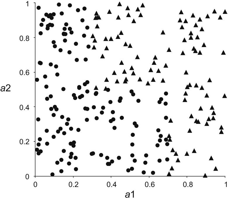
Now suppose we are trying to discretize both attributes with a view to learning the classes from the discretized attributes. The very best discretization splits a1 into three intervals (0 through 0.3, 0.3 through 0.7, and 0.7 through 1) and a2 into two intervals (0 through 0.5 and 0.5 through 1). Given these nominal attributes, it will be easy to learn how to tell the classes apart with a simple decision tree or rule algorithm. Discretizing a2 is no problem. For a1, however, the first and last intervals will have opposite labels (dot and triangle, respectively). The second will have whichever label happens to occur most in the region from 0.3 through 0.7 (it is in fact dot for the data in Fig. 8.4). Either way, this label must inevitably be the same as one of the adjacent labels—of course this is true whatever the class probability happens to be in the middle region. Thus this discretization will not be achieved by any method that minimizes the error counts, because such a method cannot produce adjacent intervals with the same label.
The point is that what changes as the value of a1 crosses the boundary at 0.3 is not the majority class but the class distribution. The majority class remains dot. The distribution, however, changes markedly, from 100% before the boundary to just over 50% after it. And the distribution changes again as the boundary at 0.7 is crossed, from 50% to 0%. Entropy-based discretization methods are sensitive to changes in the distribution even though the majority class does not change. Error-based methods are not.
Converting Discrete to Numeric Attributes
There is a converse problem to discretization. Some learning algorithms—notably the nearest-neighbor instance-based method and numeric prediction techniques involving regression—naturally handle only attributes that are numeric. How can they be extended to nominal attributes?
In instance-based learning, as described in Section 4.7, discrete attributes can be treated as numeric by defining the “distance” between two nominal values that are the same as 0 and between two values that are different as 1—regardless of the actual values involved. Rather than modifying the distance function, this can be achieved by an attribute transformation: replace a k-valued nominal attribute by k synthetic binary attributes, one for each value indicating whether the attribute has that value or not. If the attributes are scaled appropriately, this achieves the same effect on the distance function. The distance is insensitive to the attribute values because only “same” or “different” information is encoded, not the shades of difference that may be associated with the various possible values of the attribute. More subtle distinctions can be made if the attributes have weights reflecting their relative importance.
If the values of the attribute can be ordered, more possibilities arise. For a numeric prediction problem, the average class value corresponding to each value of a nominal attribute can be calculated from the training instances and used to determine an ordering—this technique was introduced for model trees in Section 7.3. (It is hard to come up with an analogous way of ordering attribute values for a classification problem.) An ordered nominal attribute can be replaced by an integer in the obvious way—but this implies not just an ordering but also a metric on the attribute’s values. The implication of a metric can be avoided by creating k–1 synthetic binary attributes for a k-valued nominal attribute, in the manner described earlier. This encoding still implies an ordering among different values of the attribute—adjacent values differ in just one of the synthetic attributes, whereas distant ones differ in several—but does not necessarily imply an equal distance between the attribute values.
8.3 Projections
Resourceful data miners have a toolbox full of techniques, such as discretization, for transforming data. As we emphasized in Chapter 2, Input: concepts, instances, attributes, data mining is hardly ever a matter of simply taking a dataset and applying a learning algorithm to it. Every problem is different. You need to think about the data and what it means, and examine it from diverse points of view—creatively!—to arrive at a suitable perspective. Transforming it in different ways can help you get started. In mathematics, a projection is a kind of function or mapping that transforms data in some way.
You don’t have to make your own toolbox by implementing the projections yourself. Comprehensive environments for machine learning, such as the one described in Appendix B, contain a wide range of suitable tools for you to use. You do not necessarily need a detailed understanding of how they are implemented. What you do need to understand is what the tools do and how they can be applied.
Data often calls for general mathematical transformations of a set of attributes. It might be useful to define new attributes by applying specified mathematical functions to existing ones. Two date attributes might be subtracted to give a third attribute representing age—an example of a semantic transformation driven by the meaning of the original attributes. Other transformations might be suggested by known properties of the learning algorithm. If a linear relationship involving two attributes, A and B, is suspected, and the algorithm is only capable of axis-parallel splits (as most decision tree and rule learners are), the ratio A/B might be defined as a new attribute. The transformations are not necessarily mathematical ones, but may involve world knowledge such as days of the week, civic holidays, or chemical atomic numbers. They could be expressed as operations in a spreadsheet or as functions that are implemented by arbitrary computer programs. Or you can reduce several nominal attributes to one by concatenating their values, producing a single k1×k2-valued attribute from attributes with k1 and k2 values, respectively. Discretization converts a numeric attribute to nominal, and we saw earlier how to convert in the other direction too.
As another kind of transformation, you might apply a clustering procedure to the dataset and then define a new attribute whose value for any given instance is the cluster that contains it using an arbitrary labeling for clusters. Alternatively, with probabilistic clustering, you could augment each instance with its membership probabilities for each cluster, including as many new attributes as there are clusters.
Sometimes it is useful to add noise to data, perhaps to test the robustness of a learning algorithm. To take a nominal attribute and change a given percentage of its values. To obfuscate data by renaming the relation, attribute names, and nominal and string attribute values—because it is often necessary to anonymize sensitive datasets. To randomize the order of instances or produce a random sample of the dataset by resampling it. To reduce a dataset by removing a given percentage of instances, or all instances that have certain values for nominal attributes, or numeric values above or below a certain threshold. Or to remove outliers by applying a classification method to the dataset and deleting misclassified instances.
Different types of input call for their own transformations. If you can input sparse data files (see Section 2.4), you may need to be able to convert datasets to nonsparse form, and vice versa. Textual input and time series input call for their own specialized conversions, described in the subsections that follow. But first we look at general techniques for transforming data with numeric attributes into a lower-dimensional form that may be more useful for mining.
Principal Component Analysis
In a dataset with k numeric attributes, you can visualize the data as a cloud of points in k-dimensional space—the stars in the sky, a swarm of flies frozen in time, a two-dimensional scatter plot on paper. The attributes represent the coordinates of the space. But the axes you use, the coordinate system itself, is arbitrary. You can place horizontal and vertical axes on the paper and represent the points of the scatter plot using those coordinates, or you could draw an arbitrary straight line to represent the x-axis and one perpendicular to it to represent y. To record the positions of the flies you could use a conventional coordinate system with a north–south axis, an east–west axis, and an up–down axis. But other coordinate systems would do equally well. Creatures like flies don’t know about north, south, east and west, although, being subject to gravity, they may perceive up–down as something special. And as for the stars in the sky, who’s to say what the “right” coordinate system is?
Back to the dataset. Just as in these examples, there is nothing to stop you transforming all the data points into a different coordinate system. But unlike these examples, in data mining there often is a preferred coordinate system, defined not by some external convention but by the very data itself. Whatever coordinates you use, the cloud of points has a certain variance in each direction, indicating the degree of spread around the mean value in that direction. It is a curious fact that if you add up the variances along each axis and then transform the points into a different coordinate system and do the same there, you get the same total variance in both cases. This is always true provided the coordinate systems are orthogonal, i.e., each axis is at right angles to the others.
The idea of principal component analysis is to use a special coordinate system that depends on the cloud of points as follows: place the first axis in the direction of greatest variance of the points to maximize the variance along that axis. The second axis is perpendicular to it. In two dimensions there is no choice—its direction is determined by the first axis—but in three dimensions it can lie anywhere in the plane perpendicular to the first axis, and in higher dimensions there is even more choice, though it is always constrained to be perpendicular to the first axis. Subject to this constraint, choose the second axis in the way that maximizes the variance along it. And so on, choosing each axis to maximize its share of the remaining variance.
How do you do this? It’s not hard, given an appropriate computer program, and it’s not hard to understand, given the appropriate mathematical tools. Technically—for those who understand the italicized terms—you calculate the covariance matrix of the original coordinates of the points and diagonalize it to find the eigenvectors. These are the axes of the transformed space, sorted in order of eigenvalue—because each eigenvalue gives the variance along its axis.
Fig. 8.5 shows the result of transforming a particular dataset with 10 numeric attributes, corresponding to points in 10-dimensional space. Imagine the original dataset as a cloud of points in 10 dimensions—we can’t draw it! Choose the first axis along the direction of greatest variance, the second perpendicular to it along the direction of next greatest variance, and so on. The table gives the variance along each new coordinate axis in the order in which the axes were chosen. Because the sum of the variances is constant regardless of the coordinate system, they are expressed as percentages of that total. We call axes components and say that each one “accounts for” its share of the variance. Fig. 8.5B plots the variance that each component accounts for against the component’s number. You can use all the components as new attributes for machine learning, or you might want to choose just the first few, the principal components, and discard the rest. In this case, three principal components account for 84% of the variance in the dataset; seven account for more than 95%.

On numeric datasets it is common to use principal component analysis prior to data mining as a form of data cleanup and dimensionality reduction. For example, you might want to replace the numeric attributes with the principal component axes or with a subset of them that accounts for a given proportion—say, 95%—of the variance. Note that the scale of the attributes affects the outcome of principal component analysis, and it is common practice to standardize all attributes to zero mean and unit variance first.
Another possibility is to apply principal component analysis recursively in a decision tree learner. At each stage an ordinary decision tree learner chooses to split in a direction that is parallel to one of the axes. However, suppose a principal component transform is performed first, and the learner chooses an axis in the transformed space. This equates to a split along an oblique line in the original space. If the transform is performed afresh before each split, the result will be an oblique decision tree whose splits are in directions that are not parallel with the axes or with one another.
Random Projections
Principal component analysis transforms the data linearly into a lower-dimensional space. But it’s expensive. The time taken to find the transformation (which is a matrix comprising the eigenvectors of the covariance matrix) is cubic in the number of dimensions. This makes it infeasible for datasets with a large number of attributes. A far simpler alternative is to use a random projection of the data into a subspace with a predetermined number of dimensions. It’s very easy to find a random projection matrix. But will it be any good?
In fact, theory shows that random projections preserve distance relationships quite well on average. This means that they could be used in conjunction with kD-trees or ball trees to do approximate nearest-neighbor search in spaces with a huge number of dimensions. First transform the data to reduce the number of attributes; then build a tree for the transformed space. In the case of nearest-neighbor classification you could make the result more stable, and less dependent on the choice of random projection, by building an ensemble classifier that uses multiple random matrices.
Not surprisingly, random projections perform worse than ones carefully chosen by principal component analysis when used to preprocess data for a range of standard classifiers. However, experimental results have shown that the difference is not too great—and it tends to decrease as the number of dimensions increases. And of course, random projections are far cheaper computationally.
Partial Least Squares Regression
As mentioned earlier, principal component analysis is often performed as a preprocessing step before applying a learning algorithm. When the learning algorithm is linear regression, the resulting model is known as principal component regression. Since principal components are themselves linear combinations of the original attributes, the output of principal component regression can be re-expressed in terms of the original attributes. In fact, if all the components are used—not just the “principal” ones—the result is the same as that obtained by applying least squares regression to the original input data. Using fewer than the full set of components results in a reduced regression.
Partial least squares differs from principal component analysis in that it takes the class attribute into account, as well as the predictor attributes, when constructing a coordinate system. The idea is to calculate derived directions that, as well as having high variance, are strongly correlated with the class. This can be advantageous when seeking as small a set of transformed attributes as possible to use for supervised learning.
There is a simple iterative method for computing the partial least squares directions that involves only dot product operations. Starting with input attributes that have been standardized to have zero mean and unit variance, the attribute coefficients for the first partial least squares direction are found by taking the dot product between each attribute vector and the class vector in turn. To find the second direction the same approach is used, but the original attribute values are replaced by the difference between the attribute’s value and the prediction from a simple univariate regression that uses the first direction as the single predictor of that attribute. These differences are called residuals. The process continues in the same fashion for each remaining direction, with residuals for the attributes from the previous iteration forming the input for finding the current partial least squares direction.
Here is a simple worked example that should help make the procedure clear. For the first five instances from the CPU performance data in Table 1.5, Table 8.1A shows the values of CHMIN and CHMAX (after standardization to zero mean and unit variance) and PRP (not standardized). The task is to find an expression for the target attribute PRP in terms of the other two. The attribute coefficients for the first partial least squares direction are found by taking the dot product between the class and each attribute in turn. The dot product between the PRP and CHMIN columns is –0.4472, and that between PRP and CHMAX is 22.981. Thus the first partial least squares direction is
Table 8.1
The First Five Instances From the CPU Performance Data; (A) Original Values; (B) The First Partial Least Squares Direction; (C) Residuals From the First Direction
| (A) | (B) | (C) | |||||
| CHMIN | CHMAX | PRP | PLS1 | CHMIN | CHMAX | PRP | |
| 1 | 1.7889 | 1.7678 | 198 | 39.825 | 0.0436 | 0.0008 | 198 |
| 2 | −0.4472 | −0.3536 | 269 | −7.925 | −0.0999 | −0.0019 | 269 |
| 3 | −0.4472 | −0.3536 | 220 | −7.925 | −0.0999 | −0.0019 | 220 |
| 4 | −0.4472 | −0.3536 | 172 | −7.925 | −0.0999 | −0.0019 | 172 |
| 5 | −0.4472 | −0.7071 | 132 | −16.05 | 0.2562 | 0.005 | 132 |

Table 8.1B shows the values for PLS1 obtained from this formula.
The next step is to prepare the input data for finding the second partial least squares direction. To this end PLS1 is regressed onto CHMIN and CHMAX in turn, resulting in linear equations that predict each of these attributes individually from PLS1. The coefficients are found by taking the dot product between PLS1 and the attribute in question, and dividing the result by the dot product between PLS1 and itself. The resulting univariate regression equations are:
Table 8.1C shows the CPU data in preparation for finding the second partial least squares direction. The original values of CHMIN and CHMAX have been replaced by residuals, i.e., the difference between the original value and the output of the corresponding univariate regression equation given above (the target value PRP remains the same). The entire procedure is repeated using this data as input to yield the second partial least squares direction, which is
After this last partial least squares direction has been found, the attribute residuals are all-zero. This reflects the fact that, as with principal component analysis, the full set of directions account for all of the variance in the original data.
When the partial least squares directions are used as input to linear regression, the resulting model is known as a partial least squares regression model. As with principal component regression, if all the directions are used, the solution is the same as that obtained by applying linear regression to the original data.
Independent Component Analysis
Principal component analysis finds a coordinate system for a feature space that captures the covariance of the data. In contrast, independent component analysis seeks a projection that decomposes the data into sources that are statistically independent.
Consider the “cocktail party problem,” where people hear music and the voices of other people: the goal is to un-mix these signals. Of course, there are many other scenarios where a linear mixing of information must be unscrambled. Independent component analysis finds a linear projection of the mixed signal that gives the most statistically independent set of transformed variables.
Principal component analysis is sometimes thought of as seeking to transform correlated variables into linearly uncorrelated variables. However, correlation and statistical independence are two different criteria. Uncorrelated variables have correlation coefficients of zero, corresponding to zero entries in a covariance matrix. Two variables are considered independent when their joint probability is the product of their marginal probabilities. (We will discuss marginal probabilities in Section 9.1.)
A quantity called mutual information measures the amount of information one can obtain from one random variable given another. It can be used as an alternative criterion for finding a projection of data, based on minimizing the mutual information between the dimensions of the data in a linearly transformed space. Given a model s=Ax, where A is an orthogonal matrix, x is the input data and s is the decomposition into the source signals, it can be shown that minimizing the mutual information between the dimensions of s corresponds to transforming the data so that the estimated probability distribution of the sources p(s) is as far from Gaussian as possible and the estimates s are constrained to be uncorrelated.
A popular technique for performing independent component analysis known as fast ICA uses a quantity known as the negentropy J(s)=H(z)−H(s), where z is a Gaussian random variable with the same covariance variance matrix as s and H(.) is the “differential entropy,” defined as
Negentropy measures the departure of s’s distribution from the Gaussian distribution. Fast ICA uses simple approximations to the negentropy allowing learning to be performed more quickly.
Linear Discriminant Analysis
Linear discriminant analysis is another way of finding a linear transformation of data that reduces the number of dimensions required to represent it. It is often used for dimensionality reduction prior to classification, but can also be used as a classification technique itself. Unlike principal and independent component analysis, it uses labeled data. The data is modeled by a multivariate Gaussian distribution for each class c, with mean ![]() and a common covariance matrix
and a common covariance matrix ![]() . Because the covariance matrix for each class is assumed to be the same, the posterior distribution over the classes has a linear form, and for each class a linear discriminant function
. Because the covariance matrix for each class is assumed to be the same, the posterior distribution over the classes has a linear form, and for each class a linear discriminant function ![]() is computed, where nc is the number of examples of class c and n the total number of examples. The data is classified by choosing the largest yc. Appendix A.2 gives more information about multivariate Gaussian distributions.
is computed, where nc is the number of examples of class c and n the total number of examples. The data is classified by choosing the largest yc. Appendix A.2 gives more information about multivariate Gaussian distributions.
Quadratic Discriminant Analysis
Quadratic discriminant analysis is obtained simply by giving each class its own covariance matrix ![]() and mean
and mean ![]() . The decision boundaries defined by the posterior probability over classes will be described by quadratic equations. The quadratic discriminant functions for each class c are
. The decision boundaries defined by the posterior probability over classes will be described by quadratic equations. The quadratic discriminant functions for each class c are
where these functions are produced by taking the log of the corresponding Gaussian model for each class and ignoring the constant terms, since such functions will be compared with one another.
Fisher’s Linear Discriminant Analysis
Linear discriminant analysis of the form discussed above has its roots in an approach developed by the famous statistician R.A. Fisher, who arrived at linear discriminants from a different perspective. He was interested in finding a linear projection for data that maximizes the variance between classes relative to the variance for data from the same class. This approach is known as Fisher’s linear discriminant analysis, and can be formulate for two classes or multiple classes.
In the two-class case, we seek a projection vector a that can be used to compute scalar projections y=ax for input vectors x. It is obtained by computing the means of each class, ![]() and
and ![]() in the usual way. Then the between-class scatter matrix
in the usual way. Then the between-class scatter matrix ![]() is calculated (note the use of the outer product of two vectors here, which gives a matrix, rather than the dot product used earlier in the book, which gives a scalar); along with the within-class scatter matrix
is calculated (note the use of the outer product of two vectors here, which gives a matrix, rather than the dot product used earlier in the book, which gives a scalar); along with the within-class scatter matrix
a is found by maximizing the “Rayleigh quotient”
This leads to the solution ![]() . The difference between principal component analysis and Fisher’s linear discriminant analysis is nicely visualized in Fig. 8.6, which shows the 1-dimensional linear projection obtained by both methods for a two-class problem in two dimensions.
. The difference between principal component analysis and Fisher’s linear discriminant analysis is nicely visualized in Fig. 8.6, which shows the 1-dimensional linear projection obtained by both methods for a two-class problem in two dimensions.

With more than two classes, the problem is to find a projection matrix A for which the low-dimensional projection given by y=ATx yields a cloud of points that are close when they are in the same class relative to the overall spread. To do this, compute the mean ![]() for each class and the global mean
for each class and the global mean ![]() , and then find the within- and between-class scatter matrices
, and then find the within- and between-class scatter matrices
A is the matrix that maximizes
This ratio of determinants is a generalization of the ratio J(a) used above. Determinants serve as analogs of variances computed in multiple dimensions and multiplied together, but computed along the principal directions of the scatter matrices.
Solving this requires sophisticated linear algebra. The idea is to construct something known as a “generalized eigenvalue problem” for each column of the matrix A. The columns of the optimal A are the generalized eigenvectors ai corresponding to the largest eigenvalues ![]() for the equation
for the equation ![]() . (Appendix A.1 gives more information about eigenvalues and eigenvectors.) It has been shown that solutions have the form
. (Appendix A.1 gives more information about eigenvalues and eigenvectors.) It has been shown that solutions have the form ![]() , where U is obtained from the eigenvectors of
, where U is obtained from the eigenvectors of ![]() .
.
Fisher’s linear discriminant analysis is quite popular for achieving dimensionality reduction, but for C classes it is limited to finding at most a C–1 dimensional projection. The Further reading section at the end of this chapter discusses a variant that can go beyond C–1 dimensions and provide non-linear projections as well.
The above analysis is based on the use of means and scatter matrices, but does not assume an underlying Gaussian distribution as ordinary linear discriminant analysis does. Of course, logistic regression, described in Section 4.6, is an even more direct way to create a linear binary classifier. Logistic regression is one of the most popular methods of applied statistics; we discuss the multiclass version in Section 9.7.
Text to Attribute Vectors
In Section 2.4 we introduced string attributes that contain pieces of text and remarked that the value of a string attribute is often an entire document. String attributes are basically nominal, with an unspecified number of values. If they are treated simply as nominal attributes, models can be built that depend on whether the values of two string attributes are equal or not. But that does not capture any internal structure of the string or bring out any interesting aspects of the text it represents.
You could imagine decomposing the text in a string attribute into paragraphs, sentences, or phrases. Generally, however, the word is the most useful unit. The text in a string attribute is usually a sequence of words, and is often best represented in terms of the words it contains. For example, you might transform the string attribute into a set of numeric attributes, one for each word, that represent how often the word appears. The set of words—i.e., the set of new attributes—is determined from the dataset and is typically quite large. If there are several string attributes whose properties should be treated separately, the new attribute names must be distinguished, perhaps by a user-determined prefix.
Conversion into words—tokenization—is not such a simple operation as it sounds. Tokens may be formed from contiguous alphabetic sequences with nonalphabetic characters discarded. If numbers are present, numeric sequences may be retained too. Numbers may involve + or − signs, may contain decimal points, and may have exponential notation—in other words, they must be parsed according to a defined number syntax. An alphanumeric sequence may be regarded as a single token. Perhaps the space character is the token delimiter; perhaps whitespace (including the tab and new-line characters), and perhaps punctuation is too. Periods can be difficult: sometimes they should be considered part of the word (e.g., with initials, titles, abbreviations, and numbers), but sometimes they should not (e.g., if they are sentence delimiters). Hyphens and apostrophes are similarly problematic.
All words may be converted to lower case before being added to the dictionary. Words on a fixed, predetermined list of function words or stopwords—such as the, and, and but—could be ignored. Note that stopword lists are language dependent. In fact, so are capitalization conventions (German capitalizes all nouns), number syntax (Europeans use the comma for a decimal point), punctuation conventions (Spanish has an initial question mark), and, of course, character sets. Text is complicated!
Low frequency words such as hapax legomena1 are often discarded too. Sometimes it is found beneficial to keep the most frequent k words after stopwords have been removed—or perhaps the top k words for each class.
Along with all these tokenization options, there is also the question of what the value of each word attribute should be. The value may be the word count—the number of times the word appears in the string—or it may simply indicate the word’s presence or absence. Word frequencies could be normalized to give each document’s attribute vector the same Euclidean length. Alternatively, the frequencies fij for word i in document j can be transformed in various standard ways. One standard logarithmic term frequency measure is log (1+fij). A measure that is widely used in information retrieval is TF×IDF, or “term frequency times inverse document frequency.” Here, the term frequency is modulated by a factor that depends on how commonly the word is used in other documents. The TF×IDF metric is typically defined as
The idea is that a document is basically characterized by the words that appear often in it, which accounts for the first factor, except that words used in every document or almost every document are useless as discriminators, which accounts for the second. TF×IDF is used to refer not just to this particular formula but to a general class of measures of the same type. For example, the frequency factor fij may be replaced by a logarithmic term such as log (1+fij).
Time Series
In time series data, each instance represents a different time step and the attributes give values associated with that time—such as in weather forecasting or stock market prediction. You sometimes need to be able to replace an attribute’s value in the current instance by the corresponding value in some other instance in the past or the future. Even more common is to replace an attribute’s value by the difference between the current value and the value in some previous instance. For example, the difference—often called the Delta—between the current value and the preceding one is often more informative than the value itself. The first instance, for which the time-shifted value is unknown, may be removed, or replaced with a missing value. The Delta value is essentially the first derivative scaled by some constant that depends on the size of the time step. Successive Delta transformations take higher derivatives.
In some time series, instances do not represent regular samples, but the time of each instance is given by a timestamp attribute. The difference between timestamps is the step size for that instance, and if successive differences are taken for other attributes they should be divided by the step size to normalize the derivative. In other cases each attribute may represent a different time, rather than each instance, so that the time series is from one attribute to the next rather than one instance to the next. Then, if differences are needed, they must be taken between one attribute’s value and the next attribute’s value for each instance.
8.4 Sampling
In many applications involving a large volume of data it is necessary to come up with a random sample of much smaller size for processing. A random sample is one in which each instance in the original dataset has an equal chance of being included. Given a batch of N instances, a sample of any desired size is easily created: just generate uniform random integers between 1 and N and retrieve the corresponding instances until the appropriate number has been collected. This is sampling with replacement, because the same instance might be selected more than once. (In fact, we used sampling with replacement for the bootstrap algorithm in Section 5.4.) For sampling without replacement, simply note when selecting each instance whether it has already been chosen and, if so, discard the second copy. If the sample size is much smaller than the full dataset there is little difference between sampling with and without replacement.
Reservoir Sampling
Sampling is such a simple procedure that it merits little discussion or explanation. But there is a situation in which producing a random sample of a given size becomes a little more challenging. What if the training instances arrive one by one, but the total number of them—the value of N—is not known in advance? Or suppose we need to be able to run a learning algorithm on a sample of a given size from a continuous stream of instances at any time, without repeatedly performing an entire sampling operation? Or perhaps the number of training instances is so vast that it is impractical to store them all before taking a sample?
All these situations call for a way of generating a random sample of an input stream without storing all the instances up and waiting for the last one to arrive before beginning the sampling procedure. Is it possible to generate a random sample of a given size and still guarantee that each instance has an equal chance of being selected? The answer is yes. Furthermore, there is a simple algorithm to do so.
The idea is to use a “reservoir” of size r, the size of the sample that is to be generated. To begin, place successive instances from the input stream in the reservoir until it is full. If the stream were to stop there, we would have the trivial case of a random sample of size r from an input stream of the same size. But most likely more instances will come in. The next one should be included in the sample with probability r/(r+1)—in fact, if the input stream were to stop there (N=r+1) any instance should be in the sample with this probability. Consequently, with probability r/(r+1) we replace a random instance in the reservoir with this new instance. And we carry on in the same vein, replacing a random reservoir element with the next instance with probability r/(r+2) and so on. In general, the ith instance in the input stream is placed into the reservoir at a random location with probability r/i. It is easy to show by induction that once this instance has been processed the probability of any particular instance being in the reservoir is just the same, namely r/i. Thus at any point in the procedure, the reservoir contains a random sample of size r from the input stream. You can stop at any time, secure in the knowledge that the reservoir contains the desired random sample.
This method samples without replacement. Sampling with replacement is a little harder—although for large datasets and small reservoirs there is little difference between the two. But if you really want a sample of size r with replacement, you could set up r independent reservoirs, each with size 1. Run the algorithm concurrently for all of these, and at any time their union is a random sample with replacement.
8.5 Cleansing
A problem that plagues practical machine learning is poor quality of the data. Errors in large databases are extremely common. Attribute values, and class values too, are frequently unreliable and corrupted. Although one way of addressing this problem is to painstakingly check through the data, machine learning techniques themselves can sometimes help to solve the problem.
Improving Decision Trees
It is a surprising fact that decision trees induced from training data can often be simplified, without loss of accuracy, by discarding misclassified instances from the training set, relearning, and then repeating until there are no misclassified instances. Experiments on standard datasets have shown that this hardly affects the classification accuracy of C4.5, a standard decision tree induction scheme. In some cases it improves slightly; in others it deteriorates slightly. The difference is rarely statistically significant—and even when it is, the advantage can go either way. What the technique does affect is decision tree size. The resulting trees are invariably smaller than the original ones, even though they perform about the same.
What is the reason for this? When a decision tree induction method prunes away a subtree, it applies a statistical test that decides whether that subtree is “justified” by the data. The decision to prune accepts a small sacrifice in classification accuracy on the training set in the belief that this will improve test-set performance. Some training instances that were classified correctly by the unpruned tree will now be misclassified by the pruned one. In effect, the decision has been taken to ignore these training instances.
But that decision has only been applied locally, in the pruned subtree. Its effect has not been allowed to percolate further up the tree, perhaps resulting in different choices being made of attributes to branch on. Removing the misclassified instances from the training set and relearning the decision tree is just taking the pruning decisions to their logical conclusion. If the pruning strategy is a good one, this should not harm performance. And it may improve it by allowing better attribute choices to be made.
It would no doubt be even better to consult a human expert. Misclassified training instances could be presented for verification, and those that were found to be wrong could be deleted—or better still, corrected.
Notice that we are assuming that the instances are not misclassified in any systematic way. If instances are systematically corrupted in both training and test sets—e.g., one class value might be substituted for another—it is only to be expected that training on the erroneous training set will yield better performance on the (also erroneous) test set.
Interestingly enough, it has been shown that when artificial noise is added to attributes (rather than to classes), test-set performance is improved if the same noise is added in the same way to the training set. In other words, when attribute noise is the problem it is not a good idea to train on a “clean” set if performance is to be assessed on a “dirty” one. A learning scheme can learn to compensate for attribute noise, in some measure, if given a chance. In essence, it can learn which attributes are unreliable, and, if they are all unreliable, how best to use them together to yield a more reliable result. To remove noise from attributes for the training set denies the opportunity to learn how best to combat that noise. But with class noise (rather than attribute noise), it is best to train on noise-free instances if possible.
Robust Regression
The problems caused by noisy data have been known in linear regression for years. Statisticians often check data for outliers and remove them manually. In the case of linear regression, outliers can be identified visually—although it is never completely clear whether an outlier is an error or just a surprising, but correct, value. Outliers dramatically affect the usual least-squares regression because the squared distance measure accentuates the influence of points far away from the regression line.
Statistical methods that address the problem of outliers are called robust. One way of making regression more robust is to use an absolute-value distance measure instead of the usual squared one. This weakens the effect of outliers. Another possibility is to try to identify outliers automatically and remove them from consideration. For example, one could form a regression line and then remove from consideration those 10% of points that lie furthest from the line. A third possibility is to minimize the median (rather than the mean) of the squares of the divergences from the regression line. It turns out that this estimator is very robust and actually copes with outliers in the X-direction as well as outliers in the Y-direction—which is the normal direction one thinks of outliers.
A dataset that is often used to illustrate robust regression is a graph of international telephone calls made from Belgium during the years 1950 to 1973, shown in Fig. 8.7. This data is taken from the Belgian Statistical Survey published by the Ministry of Economy. The plot seems to show an upward trend over the years, but there is an anomalous group of points from 1964 to 1969. It turns out that during this period, results were mistakenly recorded as the total number of minutes of the calls. The years 1963 and 1970 are also partially affected. This error causes a large fraction of outliers in the Y-direction.

Not surprisingly, the usual least-squares regression line is seriously affected by this anomalous data. However, the least median of squares line remains remarkably unperturbed. This line has a simple and natural interpretation. Geometrically, it corresponds to finding the narrowest strip covering half of the observations, where the thickness of the strip is measured in the vertical direction—this strip is marked gray in Fig. 8.7. The least median of squares line lies at the exact center of this band. Note that this notion is often easier to explain and visualize than the normal least-squares definition of regression. Unfortunately, there is a serious disadvantage to median-based regression techniques: they incur high computational cost, which often makes them infeasible for practical problems.
Detecting Anomalies
A serious problem with any form of automatic detection of apparently incorrect data is that the baby may be thrown out with the bathwater. Short of consulting a human expert, there is no way of telling whether a particular instance really is an error or whether it just does not fit the type of model that is being applied. In statistical regression, visualizations help. It will usually be visually apparent, even to the nonexpert, if the wrong kind of curve is being fitted—a straight line is being fitted to data that lies on a parabola, e.g., The outliers in Fig. 8.7 certainly stand out to the eye. But most classification problems cannot be so easily visualized: the notion of “model type” is more subtle than a regression line. And although it is known that good results are obtained on most standard datasets by discarding instances that do not fit a decision tree model, this is not necessarily of great comfort when dealing with a particular new dataset. The suspicion will remain that perhaps the new dataset is simply unsuited to decision tree modeling.
One solution that has been tried is to use several different learning schemes—such as a decision tree, and a nearest-neighbor learner, and a linear discriminant function—to filter the data. A conservative approach is to ask that all three schemes fail to classify an instance correctly before it is deemed erroneous and removed from the data. In some cases, filtering the data in this way and using the filtered data as input to a final learning scheme gives better performance than simply using the three learning schemes and letting them vote on the outcome. Training all three schemes on the filtered data and letting them vote can yield even better results. However, there is a danger to voting techniques: some learning algorithms are better suited to certain types of data than others, and the most appropriate scheme may simply get out-voted! We will examine a more subtle method of combining the output from different classifiers, called stacking, in Chapter 12, Ensemble learning. The lesson, as usual, is to get to know your data and look at it in many different ways.
One possible danger with filtering approaches is that they might conceivably just be sacrificing instances of a particular class (or group of classes) to improve accuracy on the remaining classes. Although there are no general ways to guard against this, it has not been found to be a common problem in practice.
Finally, it is worth noting once again that automatic filtering is a poor substitute for getting the data right in the first place. And if this is too time-consuming and expensive to be practical, human inspection could be limited to those instances that are identified by the filter as suspect.
One-Class Learning
In most classification problems, training data is available for all classes that can occur at prediction time, and the learning algorithm uses the data for the different classes to determine decision boundaries that discriminate between them. However, some problems exhibit only a single class of instances at training time, while at prediction time new instances with unknown class labels can belong either to this target class or to a new class that was not available during training. Then, two different predictions are possible: target, meaning that an instance belongs to the class experienced during training, and unknown, where the instance does not appear to belong to that class. This type of learning problem is known as one-class classification.
In many cases, one-class problems can be reformulated into two-class ones because there is data from other classes that can be used for training. However, there are genuine one-class applications where it is impossible or inappropriate to make use of negative data during training. For example, consider password hardening, a biometric system that strengthens a computer login process by not only requiring the correct password to be typed, but also that it be typed with the correct rhythm. This is a one-class problem; a single user must be verified and during training time only data from that user is available—we cannot ask anyone else to provide data without supplying them with the password!
Even in applications where instances from several classes are available at training time, it may be best to focus solely on the target class under consideration—if, e.g., new classes may occur at prediction time that differ from all those available during training. Continuing with the typing-rhythm scenario, suppose we are to recognize typists in a situation where the text is not fixed—the current typist is to be verified as who he or she claims to be from their rhythmic patterns on a block of free text. This task is fundamentally different from distinguishing one user from a group of other users, because we must be prepared to refuse attackers that the system has never seen before.
Outlier Detection
One-class classification is often called outlier (or novelty) detection because the learning algorithm is being used to differentiate between data that appears normal and abnormal with respect to the distribution of the training data. Earlier in this section we talked about making regression more robust by replacing the usual squared distance measure with the absolute-value one, and about trying to detect anomalies by using several different learning schemes.
A generic statistical approach to one-class classification is to identify outliers as instances that lie beyond a distance d from a given percentage p of the training data. Alternatively, a probability density can be estimated for the target class by fitting a statistical distribution, such as a Gaussian, to the training data; any test instances with a low probability value can be marked as outliers. The challenge is to identify an appropriate distribution for the data at hand. If this cannot be done one can adopt a non-parametric approach such as kernel density estimation (discussed in Section 9.3). An advantage of the density estimation approach is that the threshold can be adjusted at prediction time to obtain a suitable rate of outliers.
Multiclass classifiers can be tailored to the one-class situation by fitting a boundary around the target data and deeming instances that fall outside it to be outliers. The boundary can be generated by adapting the inner workings of existing multiclass classifiers such as support vector machines. These methods rely heavily on a parameter that determines how much of the target data is likely to be classified as outliers. If it is chosen too conservatively, data in the target class will erroneously be rejected. If it is chosen too liberally, the model will overfit and reject too much legitimate data.
Generating Artificial Data
Rather than modify the internal workings of a multiclass classifier to form a one-class decision boundary directly, another possibility is to generate artificial data for the outlier class and apply any off-the-shelf classifier. Not only does this allow any classifier to be used, but if the classifier produces class probability estimates the rejection rate can be tuned by altering the threshold.
The most straightforward approach is to generate uniformly distributed data and learn a classifier that can discriminate this from the target. However, different decision boundaries will be obtained for different amounts of artificial data: if too much is generated it will overwhelm the target class and the learning algorithm will always predict the artificial class. This problem can be avoided if the objective of learning is viewed as accurate class probability estimation rather than minimizing the classification error. For example, bagged decision trees (described in Section 12.2), which have been shown to yield good class probability estimators, can be used.
Once a class probability estimation model has been obtained in this fashion, different thresholds on the probability estimates for the target class correspond to different decision boundaries surrounding the target class. This means that, as in the density estimation approach to one-class classification, the rate of outliers can be adjusted at prediction time to yield an outcome appropriate for the application at hand.
There is one significant problem. As the number of attributes increases, it quickly becomes infeasible to generate enough artificial data to obtain adequate coverage of the instance space, and the probability that a particular artificial instance occurs inside or close to the target class diminishes to a point that makes any kind of discrimination impossible.
The solution is to generate artificial data that is as close as possible to the target class. In this case, because it is no longer uniformly distributed, the distribution of this artificial data—call this the “reference” distribution—must be taken into account when computing the membership scores for the resulting one-class model. In other words, the class probability estimates of the two-class classifier must be combined with the reference distribution to obtain membership scores for the target class.
To elaborate a little further, let T denote the target class for which we have training data and seek a one-class model, and A the artificial class, for which we generate data using a known reference distribution. What we would like to obtain is P(X|T), the density function of the target class, for any instance X—of course, we know P(X|A), the density function of the reference distribution. Assume for the moment that we know the true class probability function P(T|X). In practice, we need to estimate this function using a class probability estimator learned from the training data. A simple application of Bayes’s rule can be used to express P(X|T) in terms of P(T), P(T|X) and P(X|A):
To use this equation in practice, choose P(X|A), generate a user-specified amount of artificial data from it, label it A, and combine it with instances in the training set for the target class, labeled T. The proportion of target instances is an estimate of P(T), and a standard learning algorithm can be applied to this two-class dataset to obtain a class probability estimator P(T|X). Given that the value for P(X|A) can be computed for any particular instance X, everything is at hand to compute an estimate of the target density function P(X|T) for any instance X. To perform classification we choose an appropriate threshold, adjusted to tune the rejection rate to any desired value.
One question remains, namely, how to choose the reference density P(X|A). We need to be able to generate artificial data from it, and to compute its value for any instance X. Another requirement is that the data it generates should be close to the target class. In fact, ideally the reference density is identical to the target density, in which case P(T|X) becomes a constant function that any learning algorithm should be able to induce—the resulting two-class learning problem becomes trivial. This is unrealistic because it would require us to know the density of the target class. However, this observation gives a clue as to how to proceed: apply any density estimation technique to the target data and use the resulting function to model the artificial class. The better the match between P(X|A) and P(X|T), the easier the resulting two-class class probability estimation task becomes.
In practice, given the availability of powerful methods for class probability estimation and the relative lack of such techniques for density estimation, it may make sense to apply a simple density estimation technique to the target data first to obtain P(X|A) and then employ a state-of-the-art class probability estimation method to the two-class problem that is obtained by combining the artificial data with the data from the target class.
8.6 Transforming Multiple Classes to Binary Ones
Recall from Chapter 4, Algorithms: the basic methods, and Chapter 7, Extending instance-based and linear models, that some learning algorithms—e.g., standard support vector machines—only work with two-class problems. In most cases, sophisticated multiclass variants have been developed, but they may be very slow or difficult to implement. As an alternative, it is common practice to transform multiclass problems into multiple two-class ones: the dataset is decomposed into several two-class problems; the algorithm is run on each one; and the outputs of the resulting classifiers are combined. There are several popular techniques that implement this idea. We begin with a very simple one that we already touched on when discussing how to use linear regression for classification, and then move on to pairwise classification and more advanced techniques—error-correcting output codes and ensembles of nested dichotomies—that can often be profitably applied even when the underlying learning algorithm is able to deal with multiclass problems directly.
Simple Methods
At the beginning of the subsection on Linear classification in Section 4.6 we learned how to transform a multiclass dataset for multiresponse linear regression to perform a two-class regression for each class. The idea essentially produces several two-class datasets by discriminating each class against the union of all the other classes. This technique is commonly called the one-vs-rest method (or also, somewhat misleadingly, one-vs-all). For each class, a dataset is generated containing a copy of each instance in the original data, but with a modified class value. If the instance has the class associated with the corresponding dataset it is tagged yes; otherwise no. Then classifiers are built for each of these binary datasets, classifiers that output a confidence figure with their predictions—e.g., the estimated probability that the class is yes. During classification, a test instance is fed into each binary classifier, and the final class is the one associated with the classifier that predicts yes most confidently.
Of course, this method is sensitive to the accuracy of the confidence figures produced by the classifiers: if some classifiers have an exaggerated opinion of their own predictions, the overall result will suffer. That is why it can be important to carefully tune parameter settings in the underlying learning algorithm. For example, in standard support vector machines for classification, it is generally necessary to tune the parameter C, which provides an upper bound to the influence of each support vector and controls the closeness of fit to the training data, and the value of the kernel parameter—e.g., the size of the exponent in a polynomial kernel. This can be done based on internal cross-validation. It has been found empirically that the one-vs-rest method can be very competitive, at least in the case of kernel-based classifiers, when appropriate parameter tuning is done. Note that it may also be useful to apply techniques for calibrating confidence scores, discussed in Section 8.7: Calibrating class probabilities, to the individual two-class models.
Another simple and general method for multiclass problems is pairwise classification. Here a classifier is built for every pair of classes, using only the instances from these two classes. The output on an unknown test example is based on which class receives the most votes. This scheme generally yields accurate results in terms of classification error. It can also be used to produce probability estimates by applying a method called pairwise coupling, which calibrates the individual probability estimates from the different classifiers.
If there are k classes, pairwise classification builds a total of k(k–1)/2 classifiers. Although this sounds unnecessarily computation intensive, it is not. In fact, if the classes are evenly populated, a pairwise classifier is at least as quick to train as any other multiclass method. The reason is that each of the pairwise learning problems only involves instances pertaining to the two classes under consideration. If n instances are divided evenly among k classes, this amounts to 2n/k instances per problem. Suppose the learning algorithm for a two-class problem with n instances takes time proportional to n seconds to execute. Then the run time for pairwise classification is proportional to k(k–1)/2×2n/k seconds, which is (k–1)n. In other words, the method scales linearly with the number of classes. If the learning algorithm takes more time—say proportional to n2—the advantage of the pairwise approach becomes even more pronounced.
Error-Correcting Output Codes
The simple methods discussed above are often very effective. Pairwise classification in particular can be a very useful technique. In some cases it can improve accuracy even when the underlying learning algorithm, such as a decision tree learner, can deal with multiclass problems directly. This may be due to the fact that pairwise classification actually generates an ensemble of many classifiers. Ensemble learning is a well-known strategy for obtaining accurate classifiers, and we will discuss several ensemble learning methods in Chapter 12, Ensemble learning. It turns out that there are methods other than pairwise classification that can be used to generate an ensemble classifier by decomposing a multiclass problem into several two-class subtasks. The one we discuss next is based on error-correcting output codes.
Two-class decompositions of multiclass problems can be viewed in terms of the so-called “output codes” they correspond to. Let us revisit the simple one-vs-rest method to see what such codes look like. Consider a multiclass problem with four classes a, b, c, and d. The transformation can be visualized as shown in Table 8.2A, where yes and no are mapped to 1 and 0, respectively. Each of the original class values is converted into a 4-bit code word, 1 bit per class, and the four classifiers predict the bits independently. Interpreting the classification process in terms of these code words, errors occur when the wrong binary bit receives the highest confidence.
Table 8.2
Transforming a Multiclass Problem Into a Two-Class One: (A) Standard Method; (B) Error-Correcting Code
| (A) | Class | Class Vector | (B) | Class | Class Vector |
| a | 1 0 0 0 | a | 1 1 1 1 1 1 1 | ||
| b | 0 1 0 0 | b | 0 0 0 0 1 1 1 | ||
| c | 0 0 1 0 | c | 0 0 1 1 0 0 1 | ||
| d | 0 0 0 1 | d | 0 1 0 1 0 1 0 |

However, we do not have to use the particular code words shown. Indeed there is no reason why each class must be represented by 4 bits. Look instead at the code of Table 8.2B, where classes are represented by 7 bits. When applied to a dataset, seven classifiers must be built instead of four. To see what that might buy, consider the classification of a particular instance. Suppose it belongs to class a, and that the predictions of the individual classifiers are 1 0 1 1 1 1 1 (respectively). Obviously, comparing this code word with those in Table 8.2B, the second classifier has made a mistake: it predicted 0 instead of 1, no instead of yes. However, comparing the predicted bits with the code word associated with each class, the instance is clearly closer to a than to any other class. This can be quantified by the number of bits that must be changed to convert the predicted code word into those of Table 8.2B: the Hamming distance, or the discrepancy between the bit strings, is 1, 3, 3, and 5 for the classes a, b, c, and d, respectively. We can safely conclude that the second classifier made a mistake and correctly identify a as the instance’s true class.
The same kind of error correction is not possible with the code words of Table 8.2A, because any predicted string of 4 bits other than these four 4-bit words has the same distance to at least two of them. The output codes are not “error correcting.”
What determines whether a code is error correcting or not? Consider the Hamming distance between the code words representing different classes. The number of errors that can possibly be corrected depends on the minimum distance between any pair of code words, say d. The code can guarantee to correct up to ![]() 1-bit errors, because if this number of bits of the correct code word are flipped, it will still be the closest and will therefore be identified correctly. In Table 8.2A the Hamming distance for each pair of code words is 2. Hence, the minimum distance d is also 2, and we can correct no more than 0 errors! However, in the code of Table 8.2B the minimum distance is 4 (in fact, the distance is 4 for all pairs). That means it is guaranteed to correct 1-bit errors.
1-bit errors, because if this number of bits of the correct code word are flipped, it will still be the closest and will therefore be identified correctly. In Table 8.2A the Hamming distance for each pair of code words is 2. Hence, the minimum distance d is also 2, and we can correct no more than 0 errors! However, in the code of Table 8.2B the minimum distance is 4 (in fact, the distance is 4 for all pairs). That means it is guaranteed to correct 1-bit errors.
We have identified one property of a good error-correcting code: the code words must be well separated in terms of their Hamming distance. Because they comprise the rows of the code table, this property is called row separation. There is a second requirement that a good error-correcting code should fulfill: column separation. The Hamming distance between every pair of columns must be large, as must the distance between each column and the complement of every other column. In Table 8.2B, the seven columns are separated from one another by at least 1 bit.
Column separation is necessary because if two columns are identical (or if one is the complement of another), the corresponding classifiers will make the same errors. Error correction is weakened if the errors are correlated—in other words, if many bit positions are simultaneously incorrect. The greater the distance between columns, the more errors are likely to be corrected.
With fewer than four classes it is hard to construct a really effective error-correcting code because good row separation and good column separation cannot be achieved simultaneously. For example, with three classes there are only eight possible columns (23), four of which are complements of the other four. Moreover, columns with all zeroes or all ones provide no discrimination. This leaves just three possible columns, and the resulting code is not error correcting at all. (In fact, it is the standard “one-vs-rest” encoding.)
If there are few classes, an exhaustive error-correcting code such as the one in Table 8.2B can be built. In an exhaustive code for k classes, the columns comprise every possible k-bit string, except for complements and the trivial all-zero or all-one strings. Each code word contains 2k–1–1 bits. The code is constructed as follows: the code word for the first class consists of all ones; that for the second class has 2k–2 zeroes followed by 2k–2–1 ones; the third has 2k–3 zeroes followed by 2k–3 ones followed by 2k–3 zeroes followed by 2k–3–1 ones; and so on. The ith code word consists of alternating runs of 2k–i zeroes and ones, the last run being one short.
With more classes, exhaustive codes are infeasible because the number of columns increases exponentially and too many classifiers have to be built. In that case more sophisticated methods are employed, which can build a code with good error-correcting properties from a smaller number of columns, or random codes are used.
Error-correcting output codes do not work for local learning algorithms such as instance-based learners, which predict the class of an instance by looking at nearby training instances. In the case of a nearest-neighbor classifier, all output bits would be predicted using the same training instance. The problem can be circumvented by using different attribute subsets to predict each output bit, decorrelating the predictions.
Ensembles of Nested Dichotomies
Error-correcting output codes often produce accurate classifiers for multiclass problems. However, the basic algorithm produces classifications whereas often we would like class probability estimates as well—e.g., to perform cost-sensitive classification using the minimum expected cost approach discussed in Section 5.8. Fortunately, there is a method for decomposing multiclass problems into two-class ones that provides a natural way of computing class probability estimates, so long as the underlying two-class models are able to produce probabilities for the corresponding two-class subtasks.
The idea is to recursively split the full set of classes from the original multiclass problem into smaller and smaller subsets, while splitting the full dataset of instances into subsets corresponding to these subsets of classes. This yields a binary tree of classes. Consider the hypothetical 4-class problem discussed earlier. At the root node are the full set of classes {a, b, c, d}, which are split into disjoint subsets, say {a, c} and {b, d}, along with the instances pertaining to these two subsets of classes. The two subsets form the two successor nodes in the binary tree. These subsets are then split further into one-element sets, yielding successors {a} and {c} for the node {a, c}, and successors {b} and {d} for the node {b, d}. Once we reach one-element subsets, the splitting process stops.
The resulting binary tree of classes is called a nested dichotomy because each internal node and its two successors define a dichotomy—e.g., discriminating between classes {a, c} and {b, d} at the root node—and the dichotomies are nested in a hierarchy. We can view a nested dichotomy as a particular type of sparse output code. Table 8.3 shows the output code matrix for the example just discussed. There is one dichotomy for each internal node of the tree structure. Hence, given that the example involves three internal nodes, there are three columns in the code matrix. In contrast to the class vectors considered above, the matrix contains elements marked X that indicate that instances of the corresponding classes are simply omitted from the associated two-class learning problems.
Table 8.3
A Nested Dichotomy in the Form of a Code Matrix
| Class | Class Vector |
| a | 0 0 X |
| b | 1 X 0 |
| c | 0 1 X |
| d | 1 X 1 |
What is the advantage of this kind of output code? It turns out that, because the decomposition is hierarchical and yields disjoint subsets, there is a simple method for computing class probability estimates for each element in the original set of multiple classes, assuming two-class estimates for each dichotomy in the hierarchy. The reason is the chain rule from probability theory, which we will encounter again when discussing Bayesian networks in Section 9.2.
Suppose we want to compute the probability for class a given a particular instance x, i.e., the conditional probability P(a|x). This class corresponds to one of the four leaf nodes in the hierarchy of classes in the above example. First, we learn two-class models that yield class probability estimates for the three two-class datasets at the internal nodes of the hierarchy. Then, from the two-class model at the root node, an estimate of the conditional probability P({a, c}|x)—namely, that x belongs to either a or c—can be obtained. Moreover, we can obtain an estimate of P({a}|x, {a, c})—the probability that x belongs to a given that we already know that it belongs to either a or c—from the model that discriminates between the one-element sets {a} and {c}. Now, based on the chain rule, P({a}|x)=P({a}|{a, c}, x)×P({a, c}|x). Hence to compute the probability for any individual class of the original multiclass problem—any leaf node in the tree of classes—we simply multiply together the probability estimates collected from the internal nodes encountered when proceeding from the root node to this leaf node: the probability estimates for all subsets of classes that contain the target class.
Assuming that the individual two-class models at the internal nodes produce accurate probability estimates, there is reason to believe that the multiclass probability estimates obtained using the chain rule will generally be accurate. However, it is clear that estimation errors will accumulate, causing problems for very deep hierarchies. A more basic issue is that in the above example we arbitrarily decided on a particular hierarchical decomposition of the classes. Perhaps there is some background knowledge regarding the domain concerned, in which case one particular hierarchy may be preferable because certain classes are known to be related, but this is generally not the case.
What can be done? If there is no reason a priori to prefer any particular decomposition, perhaps all of them should be considered, yielding an ensemble of nested dichotomies. Unfortunately, for any nontrivial number of classes there are too many potential dichotomies, making an exhaustive approach infeasible. But we could consider a subset, taking a random sample of possible tree structures, building two-class models for each internal node of each tree structure (with caching of models, given that the same two-class problem may occur in multiple trees), and then averaging the probability estimates for each individual class to obtain the final estimates.
Empirical experiments show that this approach yields accurate multiclass classifiers and is able to improve predictive performance even in the case of classifiers, such as decision trees, that can deal with multiclass problems directly. In contrast to standard error-correcting output codes, the technique often works well even when the base learner is unable to model complex decision boundaries. The reason is that, generally speaking, learning is easier with fewer classes, so results become more successful the closer we get to the leaf nodes in the tree. This also explains why the pairwise classification technique described earlier works particularly well for simple models such as ones corresponding to hyperplanes: it creates the simplest possible dichotomies! Nested dichotomies appear to strike a useful balance between the simplicity of the learning problems that occur in pairwise classification—after all, the lowest-level dichotomies involve pairs of individual classes—and the power of the redundancy embodied in standard error-correcting output codes.
8.7 Calibrating Class Probabilities
Class probability estimation is obviously more difficult than classification. Given a way of generating class probabilities, classification error is minimized as long as the correct class is predicted with maximum probability. However, a method for classification does not imply a method of generating accurate probability estimates: the estimates that yield the correct classification may be quite poor when assessed according to the quadratic or informational loss discussed in Section 5.7. Yet—as we have stressed several times—it is often more important to obtain accurate conditional class probabilities for a given instance than to simply place it into one of the classes. Cost-sensitive prediction based on the minimum expected cost approach is one example where accurate class probability estimates are very useful.
Consider the case of probability estimation for a dataset with two classes. If the predicted probabilities are on the correct side of the 0.5 threshold commonly used for classification, no classification errors will be made. However, this does not mean that the probability estimates themselves are accurate. They may be systematically too optimistic—too close to either 0 or 1—or too pessimistic—not close enough to the extremes. This type of bias will increase the measured quadratic or informational loss, and will cause problems when attempting to minimize the expected cost of classifications based on a given cost matrix.
Fig. 8.8 demonstrates the effect of overoptimistic probability estimation for a two-class problem. The x-axis shows the predicted probability of the multinomial Naïve Bayes model from Section 4.2 for one of two classes in a text classification problem with about 1000 attributes representing word frequencies. The y-axis shows the observed relative frequency of the target class. The predicted probabilities and relative frequencies were collected by running a 10-fold cross-validation. To estimate relative frequencies, the predicted probabilities were first discretized into twenty ranges using equal-frequency discretization. Observations corresponding to one interval were then pooled—predicted probabilities on the one hand and corresponding 0/1 values on the other—and the pooled values are shown as the twenty points in the plot.

This kind of plot, known as a reliability diagram, shows how reliable the estimated probabilities are. For a well-calibrated class probability estimator, the observed curve will coincide with the diagonal. This is clearly not the case here. The Naïve Bayes model is too optimistic, generating probabilities that are too close to 0 and 1. This is not the only problem: the curve is quite far from the line that corresponds to the 0.5 threshold that is used for classification. This means that classification performance will be affected by the poor probability estimates that the model generates.
The fact that we seek a curve that lies close to the diagonal makes the remedy clear: systematic mis-estimation should be corrected by using post hoc calibration of the probability estimates to map the empirically observed curve into a diagonal. A coarse way of doing this is to use the data from the reliability diagram directly for calibration, and map the predicted probabilities to the observed relative frequencies in the corresponding discretization intervals. Data for this can be obtained using internal cross-validation or a holdout set, so that the actual test data remains untouched.
Discretization-based calibration is very fast. However, determining appropriate discretization intervals is not easy. With too few, the mapping is too coarse; with too many, each interval contains insufficient data for a reliable estimate of relative frequencies. However, other ways of calibrating can be devised. The key is to realize that calibrating probability estimates for two-class problems is a function estimation problem with one input—the estimated class probability—and one output—the calibrated probability. In principle, complex functions could be used to estimate the mapping—perhaps arbitrary polynomials. However, it makes sense to assume that the observed relationship is at least monotonically increasing, in which case increasing functions should be used.
Assuming that the calibration function is piecewise constant and monotonically increasing, there is an efficient algorithm that minimizes the squared error between the observed class “probabilities” (which are either 0 or 1 when no binning is applied) and the resulting calibrated class probabilities. Estimating a piecewise constant monotonically increasing function is an instance of isotonic regression, for which there is a fast algorithm based on the pair-adjacent violators (PAV) approach. The data consists of estimated probabilities and 0/1 values; assume it has been sorted according to the estimated probabilities. The basic PAV algorithm iteratively merges pairs of neighboring data points that violate the monotonicity constraint by computing their weighted mean—initially this will be the mean of 0/1 values—and using it to replace the original data points. This is repeated until all conflicts have been resolved. It can be shown that the order in which data points are merged does not affect the outcome of the process. The result is a function that increases monotonically in a stepwise fashion. This naïve algorithm is quadratic in the number of data points, but there is a clever variant that operates in linear time.
Another popular calibration method, which also presupposes a monotonic relationship, is to assume a linear relation between the log-odds of the estimated class probabilities and the target class probabilities. Here the logistic function is appropriate, and logistic regression can be used to estimate the calibration function, with the caveat that it is important to use log-odds of the estimated class probabilities rather than the raw values as the input for logistic regression.
Given that logistic regression, with only two parameters, uses a simpler model than the PAV approach, it can be more appropriate when little data is available for calibration, but with a large volume of data PAV-based calibration is generally preferable. Logistic regression has the advantage that it can easily be applied to calibrate probabilities for multiclass problems because multiclass versions of logistic regression exist. In the case of isotonic regression it is common to use the one-vs-rest method for problems with more than two classes, but pairwise coupling or ensembles of nested dichotomies—discussed in Section 8.6 above—offer an alternative.
Note that situations exist in which the relationship between the estimated and true probabilities is not monotonic. However, rather than switching to a more complex calibration method—or using discretization-based calibration, which does not assume monotonicity—this should perhaps be taken as an indication that the underlying class probability estimation method is not powerful enough for the problem at hand.
8.8 Further Reading and Bibliographic Notes
Attribute selection, under the term feature selection, has been investigated in the field of pattern recognition for decades. Backward elimination, e.g., was introduced in the early 1960s (Marill & Green, 1963). Kittler (1978) surveys the feature selection algorithms that have been developed for pattern recognition. Best-first search and genetic algorithms are standard artificial intelligence techniques (Goldberg, 1989; Winston, 1992).
The experiments that show the performance of decision tree learners deteriorating when new attributes are added are reported by John (1997), who gives a nice explanation of attribute selection. Langley and Sage (1997) showed that for an instance-based learner to reach a given performance level, the number of training instances must grow exponentially with the number of attributes. The idea of finding the smallest attribute set that carves up the instances uniquely is from Almuallin and Dietterich (1991, 1992) and was further developed by Liu and Setiono (1996). Kibler and Aha (1987) and Cardie (1993) both investigated the use of decision tree algorithms to identify features for nearest-neighbor learning; Holmes and Nevill-Manning (1995) used 1R to order features for selection. Kira and Rendell (1992) used instance-based methods to select features, leading to a scheme called RELIEF for Recursive Elimination of Features. Gilad-Bachrach, Navot, and Tishby (2004) show how this scheme can be modified to work better with redundant attributes. The correlation-based feature selection method was developed by Hall (2000).
The use of wrapper methods for feature selection is due to John, Kohavi, and Pfleger (1994) and Kohavi and John (1997), and genetic algorithms have been applied within a wrapper framework by Vafaie and DeJong (1992) and Cherkauer and Shavlik (1996). The selective Naïve Bayes learning scheme is due to Langley and Sage (1994). Guyon, Weston, Barnhill, and Vapnik (2002) present and evaluate the recursive feature elimination scheme in conjunction with support vector machines. The method of raced search was developed by Moore and Lee (1994). Gütlein, Frank, Hall, and Karwath (2009) investigate how to speed up scheme-specific selection for datasets with many attributes using simple ranking-based methods.
Dougherty, Kohavi, and Sahami (1995) give a brief account of supervised and unsupervised discretization, along with experimental results comparing the entropy-based method with equal-width binning and the 1R method. Frank and Witten (1999) describe the effect of using the ordering information in discretized attributes. Proportional k-interval discretization for Naïve Bayes was proposed by Yang and Webb (2001). The entropy-based method for discretization, including the use of the MDL stopping criterion, was developed by Fayyad and Irani (1993). The bottom-up statistical method using the χ2 test is due to Kerber (1992), and its extension to an automatically determined significance level is described by Liu and Setiono (1997). Fulton, Kasif, and Salzberg (1995) investigate the use of dynamic programming for discretization and derive the quadratic time bound for a general impurity function (e.g., entropy) and the linear one for error-based discretization. The example used for showing the weakness of error-based discretization is adapted from Kohavi and Sahami (1996), who were the first to clearly identify this phenomenon.
Principal component analysis is a standard technique that can be found in most statistics textbooks. Fradkin and Madigan (2003) analyze the performance of random projections. The algorithm for partial least squares regression is from Hastie et al. (2009). The TF×IDF metric is described by Witten et al. (1999b).
Hyvärinen and Oja (2000) created the fast ICA method. Duda et al. (2001) and Murphy (2012) explain the algebra underlying solutions to Fisher’s linear discriminant analysis. Sugiyama (2007) has extended it in two ways in a variant called “local Fisher discriminant analysis.” First, instead of means in the scatter matrix computations, he uses computations between datapoints themselves, which allows the dimensionality of the reduced representation to be increased. Second, he applies Scholköpf and Smola (2002)’s kernel trick to obtain non-linear projections.
There are many alternatives to the type of linear data projections discussed above. For example, multilayer perceptrons provide a way to learn data projections, because their hidden layers can be treated as projections of the data. Chapter 10, Deep learning, examines deep neural networks, including an approach for unsupervised dimensionality reduction based on a type of neural network known as an “autoencoder.”
The experiments on using C4.5 to filter its own training data were reported by John (1995). The more conservative approach of a consensus filter involving several different learning algorithms has been investigated by Brodley and Fried (1996). Rousseeuw and Leroy (1987) describe the detection of outliers in statistical regression, including the least median of squares method; they also present the telephone data of Fig. 8.7. It was Quinlan (1986) who noticed that removing noise from the training instance’s attributes can decrease a classifier’s performance on similarly noisy test instances, particularly at higher noise levels.
Barnett and Lewis (1994) address the general topic of outliers in statistical data, while Pearson (2005) describes the statistical approach of fitting a distribution to the target data. Schölkopf, Williamson, Smola, Shawe-Taylor, and Platt (2000) describe the use of support vector machines for novelty detection, while Abe, Zadrozny, and Langford (2006), amongst others, use artificial data as a second class. Combining density estimation and class probability estimation using artificial data is suggested as a generic approach to unsupervised learning by Hastie et al. (2009) and Hempstalk, Frank, and Witten (2008) describe it in the context of one-class classification. Hempstalk and Frank (2008) discuss the fair comparison of one-class and multiclass classification when several classes are available at training time and we want to discriminate against an entirely new class at prediction time.
Vitter (1985) explored the idea of reservoir sampling; he called the method we described algorithm R. Its computational complexity is O(N) where N is the number of instances in the stream, because a random number must be generated for every instance in order to determine whether to place it in the reservoir, and where. Vitter describes several other algorithms that improve upon R by reducing the number of random numbers that must be generated in order to produce the sample.
Rifkin and Klautau (2004) show that the one-vs-rest method for multiclass classification can work well if appropriate parameter tuning is applied. Friedman (1996) describes the technique of pairwise classification, Fürnkranz (2002) further analyzes it, and Hastie and Tibshirani (1998) extend it to estimate probabilities using pairwise coupling. Fürnkranz (2003) evaluates pairwise classification as a technique for ensemble learning. The idea of using error-correcting output codes for classification gained wide acceptance after a paper by Dietterich and Bakiri (1995); Ricci and Aha (1998) showed how to apply such codes to nearest-neighbor classifiers. Frank and Kramer (2004) introduce ensembles of nested dichotomies for multiclass problems. Dong, Frank, and Kramer (2005) considered using balanced nested dichotomies rather than unrestricted random hierarchies to reduce training time.
The importance of methods for calibrating class probability estimates is now well-established. Zadrozny and Elkan (2002) applied the PAV approach and logistic regression to calibration, and also investigated how to deal with multiclass problems. Niculescu-Mizil and Caruana (2005) compared a variant of logistic regression and the PAV-based method in conjunction with a large set of underlying class probability estimators, and found that the latter is preferable for sufficiently large calibration sets. They also found that multilayer perceptrons and bagged decision trees produce well-calibrated probabilities and do not require an extra calibration step. Stout (2008) describes a linear-time algorithm for isotonic regression based on minimizing the squared error.
8.9 Weka Implementations
• CfsSubsetEval (correlation-based attribute subset evaluator)
• ConsistencySubsetEval (measures class consistency for a given set of attributes, in the consistencySubsetEval package)
• ClassifierSubsetEval (uses a classifier for evaluating subsets of attributes, in the classifierBasedAttributeSelection package)
• SVMAttributeEval (ranks attributes according to the magnitude of the coefficients learned by a support vector machine, in the SVMAttributeEval package)
• ReliefF (instance-based approach for ranking attributes)
• WrapperSubsetEval (uses a classifier plus cross-validation)
• GreedyStepwise (forward selection and backward elimination search)
• LinearForwardSelection (forward selection with a sliding window of attribute choices at each step of the search, in the linearForwardSelection package)
• BestFirst (search method that uses greedy hill-climbing with backtracking)
• RaceSearch (uses the race search methodology, in the raceSearch package)
• Ranker (ranks individual attributes according to their evaluation)
Learning decision tables: DecisionTable
• Discretize (unsupervised and supervised versions)
• PKIDiscretize (proportional k-interval discretization)
Discriminant analysis for classification
• LDA, FLDA, and QDA (in the discriminantAnalysis package)
Discriminant analysis for dimensionality reduction
• MultiClassFLDA (in the discriminantAnalysis package)
Other pre- and postprocessing operations
• PrincipalComponents and RandomProjection
• Arithmetic operations; time-series operations; obfuscation; generating cluster membership values; adding noise; various conversions between numeric, binary, and nominal attributes; and various data cleansing operations
• PLSFilter (partial least squares transformation)
• Resampling and reservoir sampling
• MultiClassClassifier (includes many ways of handling multiclass problems with two-class classifiers, including error-correcting output codes)
• FastICA (independent component analysis, in the StudentFilters package)
• StringToWordVector (text to attribute vectors)
• END (ensembles of nested dichotomies, in the ensemblesOfNestedDichotomies package)