3.6. Structure and Motion I

We now study the structure and motion problem in detail. First, we solve the problem when the structure in known, called resection, then when the motion is known, called intersection. Then we present a linear algorithm to solve for both structure and motion using the multifocal tensors, and finally a factorization algorithm is presented. Again, refer to [24] for a more detailed treatment.

3.6.1. Resection

Problem 2 (Resection). Assume that the structure is given; that is, the object points, X_j, j = 1, … n, are given in some coordinate system. Calculate the camera matrices P_i, i = 1, … m from the images, that is, from x_ij.

The simplest solution to this problem is the classical DLT algorithm based on the fact that the camera equations

are linear in the unknown parameters, λ_j and P.

3.6.2. Intersection

Problem 3 (Intersection). Assume that the motion is given; that is, the camera matrices, P_i, i = 1, … m, are given in some coordinate system. Calculate the structure X_i, j = 1, … n from the images, that is, from x_i,j.

Consider the image of X in camera 1 and 2

Equation 3.25

which can be written in matrix form as (compared to (3.18)):

Equation 3.26

which again is linear in the unknowns, λ_i and X. This linear method can of course be extended to an arbitrary number of images.

3.6.3. Linear estimation of tensors

We are now able to solve the structure and motion problem given in Problem 1. The general scheme is as follows:

The eight-point algorithm

Each point correspondence gives one linear constraint on the components of the bifocal tensor according to the bifocal constraint:

Each pair of corresponding points gives a linear homogeneous constraint on the nine tensor components F_ij. Thus, given at least eight corresponding points, we can solve linearly (e.g., by SVD) for the tensor components. After the bifocal tensor (fundamental matrix) has been calculated, it has to be factorized as , which can be done by first solving for e using Fe = 0 (i.e., finding the right nullspace to F) and then for A₁₂ by solving a linear system of equations. One solution is

which can be seen from the definition of the tensor components. In the case of noisy data, it might happen that det F ≠ 0, and the right nullspace does not exist. One solution is to solve Fe = 0 in least-squares sense using SVD. Another possibility is to project F to the closest rank-2 matrix, again using SVD. Then the camera matrices can be calculated from (3.26) and finally using intersection, (3.25), to calculate the structure.

The seven-point algorithm

A similar algorithm can be constructed for the case of corresponding points in three images.

Proposition 16. The trifocal constraint in (3.21) contains four linearly independent constraints in the tensor components .

Corollary 2. At least seven corresponding points in three views are needed in order to estimate the 27 homogeneous components of the trifocal tensor.

The main difference from the eight-point algorithm is that it is not obvious how to extract the camera matrices from the trifocal tensor components. Start with the transfer equation

which can be seen as a homography between the first two images by fixing a line in the third image. The homography is the one corresponding to the plane Π defined by the focal point of the third camera and the fixed line in the third camera. Thus, we know from (3.17) that the fundamental matrix between image 1 and image 2 obeys

where T:^J denotes the matrix obtained by fixing the index J. Since this is a linear constraint on the components of the fundamental matrix, it can easily be extracted from the trifocal tensor. Then the camera matrices P₁ and P₂ could be calculated, and finally, the entries in the third camera matrix P₃ can be recovered linearly from the definition of the tensor components in (3.22); see [27].

An advantage of using three views is that lines could be used to constrain the geometry, using (3.23), giving two linearly independent constraints for each corresponding line.

The six-point algorithm

Again, a similar algorithm can be constructed for the case of corresponding points in four images.

Proposition 17. The quadrifocal constraint in (3.24) contains 16 linearly independent constraints in the tensor components Q^ijkl.

From this proposition, it seems that five corresponding points would be sufficient to calculate the 81 homogeneous components of the quadrifocal tensor. However, the following proposition says that this is not possible.

Proposition 18. The quadrifocal constraint in (3.24) for two corresponding points contains 31 linearly independent constraints in the tensor components Q^ijkl.

Corollary 3. At least six corresponding points in three views are needed in order to estimate the 81 homogeneous components of the quadrifocal tensor.

Since one independent constraint is lost for each pair of corresponding points in four images, we get linearly independent constraints.

Again, it is not obvious how to extract the camera matrices from the trifocal tensor components. First, a trifocal tensor has to be extracted, and then a fundamental matrix and the camera matrices must be extracted. It is outside the scope of this work to give the details for this; see [27]. Also, in this case, corresponding lines can be used by looking at transfer equations for the quadrifocal tensor.

3.6.4. Factorization

A disadvantage with using multiview tensors to solve the structure and motion problem is that when many images (» 4) are available, the information in all images cannot be used with equal weight. An alternative is to use a factorization method, see [59].

Write the camera equations

for a fixed image i in matrix form as

Equation 3.27

where

The camera matrix equations for all images can now be written as

Equation 3.28

where

Observe that only contains image measurements apart from the unknown depths.

Proposition 19.

This follows from (3.28), since is a product of a 3m x 4 and a 4 × n matrix. Assume that the depths, ∧_i, are known, corresponding to affine cameras, we may use the following simple factorization algorithm:

In the perspective case, this algorithm can be extended to the iterative factorization algorithm:

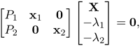
Definition 34. The fifth singular value, σ₅, in the SVD above is called the proximity measure and is a measure of the accuracy of the reconstruction. ▪

Theorem 8. The algorithm above minimizes the proximity measure.

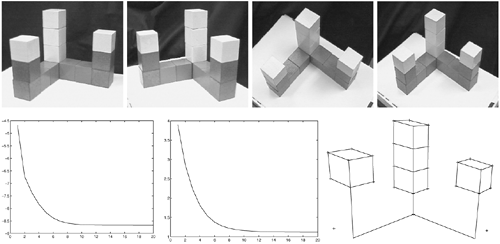
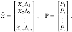
Figure 3.13 shows an example of a reconstruction using the iterative factorization method applied on four images of a toy block scene. Observe that the proximity measure decreases quite fast and the algorithm converges in about 20 steps.