
11.2. Shortest Path Computation
Given the graph of a network with a distance (cost) assigned to each link, shortest path algorithms find the least cost path between a selected node and all other nodes in the network [Bertsekas98, Gibbons85].
Before we delve into the applicability of this technique to optical path selection, we first need to introduce some terminology and notation. A network can be represented by a graph G = (N, A), where N is the set of nodes (also called vertices) and A is the set of links. (i, j)∊ A, if there is a link from node i to node j. Note that for complete generality, each link is considered to be unidirectional. If a link from node i to node j is bi-directional, then (i, j)∊ A and (j, i)∊ A. For a link (i, j)∊ A, the cost of the link is denoted by ai,j. Given two nodes s and t, a shortest path algorithm finds a path P with s as the start node and t as the termination node such that ![]() is minimized.
is minimized.
At a first glance, the shortest path technique may seem rather limited in its optimization capabilities. Different measures of path performance, how-ever, can be optimized by appropriately setting the link costs, ai,j. In fact, one can get quite creative here and a different set of weights can be chosen for optimizing under different criteria. For example, the link weights ai,j could be set to:
Dollar cost of link (i, j), which results in the minimum cost path.
Distance in miles between i and j, which results in the shortest distance path. Such a routing criterion could be used where dollar costs are proportional to distances, which is typically the case in some types of optical transport networks.
1 for all (i, j) ∊ A, which results in a minimum hop path. This type of measure was used in the early days of data networking where queuing and processing delays dominated.
ln (pi,j), where pi,j is the probability of failure of link (i, j). Using this measure, the path with the lowest probability of failure is obtained.
–10log(Attenuationi,j), where Attenuationi,j is the optical attenuation on link (i, j). Such a link weight would be useful in transparent optical networks to determine the path with the least attenuation.
11.2.1. The Bellman-Ford Algorithm
A variant of the Bellman-Ford Algorithm was used early in the Routing Information Protocol version 2 (RIPv2) for IP routing [Malkin98]. This is an iterative algorithm that computes the shortest paths from a given node to all the other nodes in the network. In computing these paths, the algorithm assigns to each node j in each iteration k, a label ![]() Let us assume that there are a total of N nodes in the network and that the origin node is 1. Then the algorithm can be defined as follows:
Let us assume that there are a total of N nodes in the network and that the origin node is 1. Then the algorithm can be defined as follows:
Initialization
![]()
Iteration
![]()
The above algorithm has the following properties:
Given that ai,j ≥ 0 for all (i,j) ∊ A, the algorithm terminates in at most N iterations, that is,
 for some k < N and all j.
Close examination of the iteration equation above shows that in each iteration, each node is examined to see which neighbor's cost, combined with the cost of the link from that neighbor, yields the shortest cost path from node 1. Hence, for each node, the node i in the iteration that resulted in the minimum distance will be the previous hop along the shortest path from node 1. It should be noted that by substituting aj,i for ai,j in the iteration equation, the cost of the shortest path from each node to node 1, and the identity of the next hop in the path can be obtained. Clearly, if link costs are symmetrical, that is, ai,j = aj,i, then the procedure above gives the cost of the shortest path in both directions.
11.2.1.1. BELLMAN-FORD ALGORITHM EXAMPLE
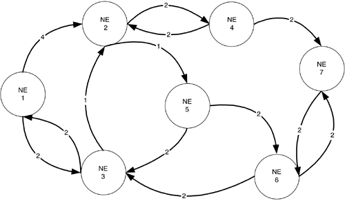
Consider the network represented by the graph shown in Figure 11-1. In this figure, the cost of a link is indicated in the middle of the link. The iterations of the Bellman-Ford algorithm are shown Table 11-1. As per the properties of the algorithm, for k = 1 we see that the shortest path from node 1 to node 2 with 1 or fewer links is simply the direct link between nodes 1 and 2. The cost of this path is 4. In the next iteration (k = 2), we get the shortest paths with two or fewer links, and it turns out that it is more cost effective to go to node 2 via node 3, rather than using the direct link. Also note that the algorithm stops before k = 7, the total number of nodes in the network.
Figure 11-1. Network Graph for Illustrating the Shortest Path Algorithm
11.2.2. Dijkstra's Algorithm
Dijkstra's algorithm [Dijkstra59] for finding shortest paths is used in what is probably the most popular intradomain IP routing protocol, OSPF [Moy98] (see Chapter 9). Like the Bellman-Ford algorithm, Dijkstra's algorithm assigns a label, di, to each node i. It, however, does not iterate over these labels. Instead, it keeps a list, V, of candidate nodes that is manipulated in its iteration procedure. Once again, without loss of generality, we will assume that we are interested in finding the shortest path from node 1 to all the other nodes in a network of N nodes.
Initialization
![]()
Iteration
Remove from V a node i such that
 .
.
| Iteration (k) | Label List (d1, …, d7), | Previous Node List (NE1, …, NE7) |
|---|---|---|
| 0 | (0, ∞, ∞, ∞, ∞, ∞, ∞) | (x, x, x, x, x, x, x) |
| 1 | (0, 4, 2, ∞, ∞, ∞, ∞) | (x, 1, 1, x, x, x, x) |
| 2 | (0, 3, 2, 6, 5, ∞, ∞) | (x, 3, 1, 2, 2, x, x) |
| 3 | (0, 3, 2, 5, 4, 7, 8) | (x, 3, 1, 2, 2, 5, 4) |
| 4 | (0, 3, 2, 5, 4, 6, 7) | (x, 3, 1, 2, 2, 5, 4) |
The algorithm above has the following properties:
Given that ai,j ≥ 0 for all (i,j)∊ A, the algorithm will terminate in at most N iterations.
All the nodes with a final label that is finite will be removed from the candidate list exactly once, in the order of increasing distance from node 1.
As the properties indicate, once a node is removed from the candidate list its distance from node 1 is known. The value of i in step (b) that led to the final value of the label indicates the previous hop in the path from 1.
11.2.2.1. DIJKSTRA'S ALGORITHM EXAMPLE
Considering the network represented by the graph in Figure 11-1 again, Table 11-2 shows the iterations of Dijkstra's algorithm. In this table, we show the labels, candidate list, and previous hop. Note that when a node is removed from the candidate list, its label and previous node value no longer change (as described by the properties). Hence, if we are only interested in getting to a particular end node rather than all possible end nodes, then we can stop the algorithm as soon as that node is removed from the candidate list.
11.2.3. A Comparison of Bellman-Ford and Dijkstra Algorithms
We described two different shortest-path algorithms in the last two sections. One might ask “which one is better?” The answer to this question depends on the context.
| Iteration | Label (d1, …, d7) | Candidate List, V | Previous Node (NE1, …, NE7) |
|---|---|---|---|
| 0 | (0, ∞, ∞, ∞, ∞, ∞, ∞) | {1}, remove 1 | (s, x, x, x, x, x, x) |
| 1 | (0, 4, 2, ∞, ∞, ∞, ∞) | {2, 3}, remove 3 | (x, 1, 1, x, x, x, x) |
| 2 | (0, 3, 2, ∞, ∞, ∞, ∞) | {2}, remove 2 | (x, 3, 1, x, x, x, x) |
| 3 | (0, 3, 2, 5, 4, ∞, ∞) | {4, 5} remove 5 | (x, 3, 1, 2, 2, x, x) |
| 4 | (0, 3, 2, 5, 4, 6, ∞) | {4, 6}, remove 4 | (x ,3, 1, 2, 2, 5, x) |
| 5 | (0, 3, 2, 5, 4, 6, 7) | {6, 7}, remove 6 | (x, 3, 1, 2, 2, 5, 4) |
| 6 | (0, 3, 2, 5, 4, 6, 7) | {7}, remove 7 | (x, 3, 1, 2, 2, 5, 4) |
Consider the distributed, asynchronous version of the Bellman-Ford algorithm used in RIPv2 [Malkin98]. It divides up the shortest path computation amongst the routers participating in the protocol. This robustness is important in the Internet. Unfortunately, with the Bellman-Ford technique, the iterations must continue until the labels stop changing. With Dijkstra's algorithm, the procedure can stop once the desired destination node(s) are removed from the candidate list. This property is useful if the paths to only a subset of nodes need to be computed. Other properties can influence the choice in particular network situations. For example, the Bellman-Ford algorithm can be significantly faster with sparse networks, that is, networks where the number of links is much less than N2, where N is the number of nodes. It was seen that when the Bellman-Ford algorithm and Dijkstra's algorithm were applied to the network of Figure 11-1, the former terminated with fewer iterations. For more information, analysis, and comparison of these algorithms, see [Bertseka98].