
11.4. Path Selection for Diversity
Multiple optical connections are often set up between the same end points, for example, working and protection connections (see Chapter 8). An important constraint on these connections is that they must be diversely routed. In particular, they may have to be routed over paths that are link diverse, that is, which do not share any common link, or node diverse, that is, which do not share any common node. Note that node diversity is a stronger criterion, and it also implies link diversity.
When multiple physical and electronic levels are considered, ensuring link diversity is complicated by the possibility of two paths being diverse at one layer but not at another. Different types of link and node diversity requirements were described in section 10.3. In the following, the computation of link diverse paths is examined.
11.4.1. Link Diverse Routing Algorithms
Suppose it is required to compute two link diverse paths between a source and a destination. A straightforward approach that could be employed is as follows. First, the shortest path between the source and the destination is computed using one of the previously described algorithms. Next, all the links in this path are pruned from the graph, and another shortest path is computed using the modified graph. By construction, these two paths will be link diverse.
11.4.1.1. NONOPTIMAL DISJOINT PATHS VIA PRUNING
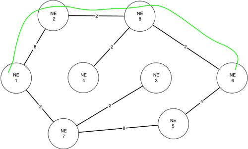
Consider the application of the pruning method to find two minimum cost link disjoint paths between NE 1 and NE 6 shown in Figure 11-6. The shortest path is computed as (NE 1, NE 4, NE 3, NE 6), with a total link cost of 3. This is indicated in the figure. The links along the shortest path are pruned from the graph to derive the graph shown in Figure 11-7. The shortest path (NE 1, NE 2, NE 8, NE 6), with a cost of 12, is then computed. This path, shown in Figure 11-7, is link-diverse from the first path.
Figure 11-6. Finding the Shortest Path

Figure 11-7. Finding the Second Link Diverse Path via the Pruned Network Graph
While the pruning approach allowed the determination of two link disjoint paths in this example, it did not incorporate a means to minimize the total cost of the two paths found. In fact, there exists two link disjoint paths whose total cost is 10 whereas the total cost of the paths found above was 15 (these paths are (NE 1, NE 4, NE 8, NE 6) and (NE 1, NE 7, NE 3, NE 6)). The pruning approach can perform much worse, as the following example shows.
Consider the network shown in Figure 11-8 in which it is desired to find two minimum cost disjoint paths from NE 1 to NE 6. The shortest path from NE 1 to NE 6 is (NE 1, NE 4, NE 3, NE 6), and it is shown in Figure 11-8. When the links in this path are pruned, the network shown in Figure 11-9 is obtained.
Figure 11-8. Network where Pruning Fails to Find Disjoint Paths

Figure 11-9. Graph of Network of Figure 11-8 with Shortest Path Links Removed

We can immediately see from this figure that we have a problem. In particular, the network is no longer connected, and hence a second path from NE 1 to NE 6 cannot be found. Two link disjoint paths, (NE 1, NE 2, NE 3, NE 6) and (NE 1, NE 4, NE 5, NE 6), indeed exist, but the pruning approach cannot be used to find them.
11.4.2. Shortest Link Diverse Paths Algorithm
The two previous examples have shown that the pruning technique does not guarantee the discovery of either the optimal or even a feasible pair of disjoint paths. A very straightforward and efficient algorithm does exist for finding a pair of link-disjoint paths with the lowest total cost [Bhandhari99]. This algorithm does not require significant additional computation as compared with the pruning method, and it is described below.
11.4.2.1. LINK DISJOINT PATH PAIR ALGORITHM
Given: A source node, s, a destination node, d, and a network represented by an undirected weighted graph with positive weights, that is, we are assuming bidirectional connections and bidirectional links.
Modify the original network graph by: (a) making each bidirectional link in S1 unidirectional in the direction from d to s, and (b) set the link weights along this direction to be the negative of the original link weights.
Compute the shortest path from s to d in the modified graph obtained in step 2. Denote the set of links in this path as S2.
Group the remaining links in S1 ∪ S2 – S3 into two disjoint paths.
Suppose we apply this algorithm on the network shown in Figure 11-8, which also depicts the shortest path from NE 1 to NE 6. The set of links, S1, in this path are { (NE 1, NE 4), (NE 4, NE 3), (NE 3, NE 6) } . This path is modified according to step 2 above, and a new shortest path is computed on the modified graph. This is shown in Figure 11-10, with the new path highlighted. The set of links, S2, in this path are { (NE 1, NE 2), (NE 2, NE 3), (NE 3, NE 4), (NE 4, NE 5), (NE 5, NE 6) } . The set, S3, of links that are in the intersection of the two shortest paths is { (NE 4, NE 5) } . After removing this link, the set of links that remain (i.e., S1 ∪ S2 – S3), is { (NE 1, NE 2), (NE 1, NE 4), (NE 2, NE 3), (NE 4, NE 5), (NE 3, NE 6), (NE 5, NE 6) } . These links are used to form the two disjoint paths, (NE 1, NE 2, NE 3, NE 6) and (NE 1, NE 4, NE 5, NE 6). Figure 11-11 depicts these links as dashed lines, along with the two disjoint paths.
Figure 11-10. Network of Figure 11-8 Transformed, with Shortest Path Indicated

Figure 11-11. The Set of “Useful” Links Along with the Two Disjoint Paths They Generate

Let us now apply this algorithm on the network shown in Figure 11-6, which also depicts the shortest path (S1) from NE1 to NE6. This path is modified according to step 2 above, and a new shortest path (S2) is computed on the modified graph. This is shown in Figure 11-12, with the new path (NE 1, NE 7, NE 3, NE 4, NE 8, NE 6) highlighted. Now the link that is in both paths (S3) is (NE 4, NE 3). After removing this link, the set of links that remain (i.e., S1 ∪ S2 – S3) is { (NE 1, NE 7), (NE 1, NE 4), (NE 4, NE 8), (NE 7, NE 3), (NE 3, NE 6), (NE 8, NE 6) } . These links are used to form the two disjoint paths, (NE 1, NE 7, NE 3, NE 6) and (NE 1, NE 4, NE 8, NE 6). Figure 11-13 depicts these links as dashed lines, along with the two disjoint paths.
Figure 11-12. Modified Graph of the Network of Figure 11-6

Figure 11-13. The Set of “Useful” Links along with the Two Disjoint Paths Generated

A proof that the above algorithm converges and finds two diverse paths with the least total cost (if they exist) can be found in [Bhandhari99]. In both the examples given above, the two link-diverse paths were also node-diverse. This generally may not be the case. By applying additional transformations to the network graph, an algorithm for finding two node-disjoint paths of least total cost can be obtained [Bhandhari99]. Finally, it turns out that the previous algorithm can be extended to find K lowest cost link disjoint paths.