CHAPTER 6

Audio Principles of Design

In this chapter, you will learn about

•  Calculating the change in a sound and signal level using decibel equations, as well as power and distance using 10-log and 20-log functions

•  Plotting loudspeaker coverage in a room and wiring loudspeakers

•  Transformers and amplifiers

•  Different types of microphones and polar-response patterns

•  The benefits of using an automatic microphone mixer

•  The qualities of an effective sound-reinforcement system

•  Determining whether an audio system will be stable by comparing potential acoustic gain (PAG) and needed acoustic gain (NAG) calculations

Much of what you need to know as an audiovisual professional revolves around sound: how sounds are generated, how sound moves through a medium (such as air), how you might control its propagation, how sound interacts with the environment, and how you receive and process sound. As an AV designer, you need to apply math concepts and accurate measurements to support the human perception of sound as intended by your design. With an understanding of sound and sound systems, you will be better positioned to meet the needs of your clients.

For example, if you determine a loudspeaker system is necessary, your design will need to specify where the loudspeakers will be located. Your goal is to provide adequate audio coverage for listeners. To accomplish this, you will need to evaluate coverage patterns, loudspeaker locations, and power requirements.

Microphones play a vital role in ensuring your audio design supports your client’s message, giving the audience an exceptional listening environment. Special calculations, such as PAG and NAG, reduce the possibility of audio feedback within a system. PAG and NAG determinations are among the many that AV designers make when creating a stable, effective audio system design.

Introduction to the Decibel

When discussing audio, you need a way to talk about how people experience the sound that a system produces. The most common unit of measurement for sound is the decibel.

But a decibel doesn’t really measure sound. It measures change. In technical terms, a decibel is a base-10 logarithmic ratio between two values. Remember, the logarithmic scale is used to describe a large range of values, which can vary over several orders of magnitude. A ratio is just simply a comparison of two numbers. In other words, a decibel is a measurement of how much change a person will actually perceive as a linear value changes.

Before we delve further into decibels, let’s pause to discuss logarithms. The logarithm of a number is how many times the number 10 must be multiplied by itself to get a certain value. For example, the log of 10,000 is 4, and the log of 0.0001 is −4.

Logarithmic scales make ratio values easier to express. For example, the ratio between the threshold of hearing (when sounds become audible) and the threshold of pain is 1 to 1,000,000. No one wants to count that many zeros.

Think of a standard ruler. Each unit on the ruler represents a unit of 1 wherever it is located on the ruler, whether it’s an inch, millimeter, or whatever. It’s a one-to-one relationship between the units shown and the units represented. This is a linear scale.

What if the value of each unit on that ruler represented something other than a single unit? What if each time you moved to the right, each unit represented ten times as much as before? Or, each time you moved a unit to the left it represented one-tenth as much as before? In this case, comparing adjacent units on a scale would represent a ratio of 1:10 or 10:1. This is a logarithmic scale.

In Figure 6-1, the top row represents a linear scale, and the bottom row represents a logarithmic scale.

Figure 6-1    Linear and logarithmic scales

You can write 10 * 10 * 10 = 1,000 or 10³ = 1,000 (10 multiplied by itself three times). You have just used a logarithm with a base of 10 and an exponent of 3 as a shortcut for an equation that uses multiplication. Therefore, you could substitute 10¹, 10², and 10³ at the bottom of Figure 6-1 for the numbers 10, 100, and 1,000.

Humans perceive differences in sound levels logarithmically, not linearly. Because of this, a base-10 logarithmic scale is used to measure, record, and discuss sound level differences.

If you used a linear scale to describe the perceived difference in sound pressure level from the threshold of hearing to the threshold of pain, you would need to use numbers from 1 to well over 1 million.

When it comes to sounds and decibels, there are some accepted generalities related to human hearing.

•  A 1 decibel (dB) change is the smallest perceptible change noticeable. Unless they’re listening carefully, most people will not discern a 1 dB change.

•  A “just noticeable” change—either louder or softer—requires a 3 dB change (e.g., 85 dB sound pressure level [SPL] to 88 dB SPL).

•  A 10 dB change is required for listeners to perceive subjectively a sound that is twice or one-half as loud as it was before. For example, a change from 85 dB SPL to 95 dB SPL is perceived to be twice as loud.

Why Use Decibels?

Even before you got into the audiovisual industry, you probably heard sound described in decibels. Did you know that you can also use decibels to measure distance, power, and voltage? Because a decibel measures perceived change—not actual pressure or sound—you can use it to quantify many kinds of changes. For this reason, the decibel is dimensionless and cannot be properly called a unit.

A decibel change in distance, voltage, or power will result in the same decibel change in sound pressure. If you want to increase the loudness of a sound system by 5 dB, you just need to increase the power or voltage by 5 dB.

Calculating Decibel Changes

As you’ve learned, a decibel doesn’t really measure anything. It’s a ratio—a comparison of two values. To compare, you need a start point and an end point. Those values will be real measurements, in linear units such as pascals, volts, watts, or meters. They must be like units; you can compare only volts to volts, watts to watts, meters to meters, and so on. Once you’ve converted the values to decibels, you can compare them to each other.

Calculating the decibel change from one distance, voltage, or power measurement to another will tell you how much louder or softer the output of a sound system will seem after the change. To convert linear measurements, such as meters, volts, or watts, to the logarithmic decibel, you use a logarithmic equation.

To calculate the change in decibels between two power measurements, use the 10-log equation. The formula for calculating a decibel change for power is as follows:

dB = 10 * log (P₁/P_r)

where:

•  dB = The change in decibels

•  P₁ = The new or measured power measurement

•  P_r = The original or reference power measurement

The result of this formula will be either positive or negative. If it is positive, the result is an increase, or gain. If it is negative, the result is a decrease, or loss.

To calculate the change in decibels between two voltage or distance measurements, use the 20-log equation. The formula for calculating decibel changes in sound pressure level over distance is as follows:

dB = 20 * log (D₁/D₂)

where:

•  dB = The change in decibels

•  D₁ = The original or reference distance

•  D₂ = The new or measured distance

As before, the result of this calculation will be either positive or negative. If it is positive, the result is an increase, or gain. If it is negative, the result is a decrease, or loss.

The formula for calculating decibel changes in voltage is as follows:

dB = 20 * log (V₁/V_r)

where:

•  dB = The change in decibels

•  V₁ = The new or measured voltage

•  V_r = The original or reference voltage

Once again, the result of this calculation will be either positive or negative. If it is positive, the result is an increase, or gain. If it is negative, the result is a decrease, or loss.

Reference Level

A decibel can be a comparison of two values, or it can be a comparison of a value to a predetermined starting point, known as a reference level. This is also sometimes referred to as a zero reference. For example, you could compare two voltages and use a 20-log formula to discover the decibel change between them.

In the context of decibel measurements, the reference level is the established starting point, represented as 0 dB. The reference level varies according to linear unit and application. It is typically indicated by the decibel abbreviations. Table 6-1 shows decibel abbreviations and reference levels for various common measurements.

Table 6-1    Decibel Abbreviations and Reference Levels

To use a reference level as a starting point, you have to know what the reference is. For sound pressure, the reference level is the threshold of human hearing at 1 kHz, 0.00002 Pa. Humans perceive that sound pressure level as silence. Any unit you might quantify in decibels has its own reference level.

Decibels will be abbreviated differently to indicate the reference level used. For example, dB SPL indicates that the reference level is a sound pressure level of 0.00002 Pa at 1 kHz. Meanwhile, dBV indicates that the reference level is a voltage of 1 V.

Some units, such as volts and watts, have more than one zero reference. Use the one that makes sense for the application. If you’re taking power measurements at a radio station, use dBW. If you’re measuring the power of wireless microphones, use dBm.

Decibels are often qualified with a suffix. These suffixes indicate the reference quantity. Two suffixes often found in the AV industry are dBu and dBV. Both reference voltage ratios.

0 dBu is equivalent to 0.775 volts.

Pro-audio line level is often expressed as +4 dBu, which expresses a voltage above the 0.775 reference point, or 1.23 volts. If you have a microphone level of −50 dBu, that does not mean the device has “negative voltage.” Instead, it is expressing a voltage level less than the 0.775 volt reference point, or 2 millivolts.

0 dBV is equivalent to 1 volt.

The consumer line level is often expressed as −10 dBV, or 316 millivolts. A good clue that a device’s level might be −10 dBV is the use of the phono or RCA connector.

As an AV professional, you should commit certain decibel values to memory.

•  Sound pressure level should always fall between 0 and 140 dB SPL.

•  Microphone level, which is typically measured in dBu, should be −60 to −50 dBu, well below the zero reference of 0.775 volts for the dBu.

•  Line level on the other hand, should be between 0 and +4 dBu for pro audio.

•  The consumer audio level is −10 dBV (0.316 V).

Let’s try a 10-log decibel calculation. An audio amplifier is delivering 15 watts, and its output is decreased to 5 watts. What is the change in decibels?

•  Step 1    Ask yourself, “What do I expect to happen?” If the amplifier will be delivering less power, then there will be less sound coming out of the system. In the AV industry, this is called a loss.

•  Step 2    Which number do you put first? If you expect a gain, place the higher number first. If you expect a loss, place the smaller number first. In this example, you are expecting a loss, so the smaller number (5) goes first (5/15 = 0.33).

•  Step 3    Calculate the log. In this example, the problem concerns power. Therefore, you need to use the 10-log formula. In step 2, you completed the division. Now enter 0.33 in your calculator and press the “log” button.

10 * log (P₁/P₂)

10 * log (0.33)

10 * (−0.48)

•  Step 4    Multiply −0.48 by 10.

10 * (−0.48)

Answer: −4.8 dB

Sound Pressure Level

Figure 6-2 shows a graph of the equal loudness curves. These contours were formed using short-duration, pure tones. Levels shown are referenced to a 1kHz tone, which takes into account the ear’s relative insensitivity to low-frequency energy at low overall listening levels.

Figure 6-2    Fletcher-Munson equal loudness contour

The threshold of human hearing is 0 dB SPL at 1 kHz. The graph in Figure 6-2 shows how loud different frequencies must be for the human ear to perceive them as equally loud as another.

What sound pressure level would a 40 Hz tone require to be perceived equally as loud as a 1 kHz tone? The dotted curve represents the threshold of human hearing, which is what the human ear perceives. The x-axis of the graph shows actual frequency, and the y-axis shows actual dB SPL.

A 40 Hz tone must be about 50 dB SPL louder before the human ear can perceive it equally as loud as 1 kHz. A 200 Hz tone, however, would only have to be 15 dB SPL louder to be perceived equally as loud as the 1 Hz tone.

Notice that at overall louder listening levels the hearing response curve begins to flatten. Human perception of the energy across the audible spectrum is more even at overall louder listening levels. Also note that your ears’ sensitivity is where normal speech frequencies are located, 500 to 4,000 Hz. And your ears are most sensitive to higher-pitched sounds, such as a crying baby.

SPL Meters

Sound pressure level is a measurement of all the acoustic energy in an environment. It is typically expressed in decibels (dB SPL). Sound pressure refers to the pressure deviation from the ambient atmospheric pressure caused by the vibration of air particles. SPL is expressed in decibels to correlate with the human perception of changes in loudness.

An SPL meter reports a single-number measurement of the sound pressure at the meter’s microphone location. The meter has a calibrated microphone and the necessary circuitry to detect and display the sound level. Its function is simple: An SPL meter converts the sound pressure levels in the air into corresponding electrical signals. These signals are measured and processed through internal filters, and the results are displayed in decibels.

SPL Meter Settings

Always reference the project specifications to obtain the necessary SPL meter settings for properly verifying the audio performance of a system. If the verification requirements do not specify settings for the SPL meter, you can apply a weighting to the SPL meter measurements to correlate the meter’s readings with how people perceive loudness. A meter will typically have three settings.

•  A-weighting    A setting commonly used for environmental, hearing conservation, and noise ordinance enforcement. It closely reflects the response of the human ear to noise and its insensitivity to lower frequencies at lower listening levels.

•  C-weighting    More uniform response over the entire frequency range.

•  Z-weighting    A flat frequency response, with no filtering.

Historically, there used to be B-weighting (where filtering fell between the A and C weightings) and D-weighting (like for jet engines), but they are not included in the latest standards.

In addition to applying a weighting to SPL readings when verifying performance, you can select a specific response.

•  Fast, to capture transient (momentary) levels.

•  Slow, which is more like how your ears react to sound. Use this response for more consistent noise levels or for averaging rapidly changing fluctuations in sound levels.

Keep in mind, an audio system may need to comply with a standard. SPL meter performance falls under two different standards. Internationally, the standard is governed by the International Electrotechnical Commission (IEC); in the United States, it’s the American National Standards Institute (ANSI).

The IEC standard relates to frontal-incidence correction, while the ANSI standard relates to random-incidence correction. In other words, does the microphone have to be oriented directly on-axis with the noise source to be compliant (IEC), or can it be off-axis up to a certain point (ANSI)? These two different standards have more to do with the response than weighting.

SPL Meter Classes

When selecting an SPL meter, you want to use one that can take extremely accurate readings. SPL meters are classified based on allowable tolerances. Devices that are not classified do not conform to a standard and are not reliable for measurement and testing purposes. How do you know which class of meter to use for the task?

•  Class 0    A lab-reference standard. It supports the strictest tolerances and should be used when extreme precision is needed.

•  Class 1    Precision measurement. It is useful for taking flat, engineering-grade measurements, rather than wide-range or field measurements.

•  Class 2    For general purpose. It has the widest tolerances with respect to level linearity and frequency response. Class 2 meters are required only to support A-weighting. Other weightings are optional. For many audio purposes, a Class 2 meter is acceptable.

•  Class 3    Intended for noise surveys. Class 2 meters are simple SPL meters meant to determine whether a noise problem exists. If a problem does exist, diagnosing it will require a higher-class meter.

SPL Meter Weighting Curves

You can see the differences in SPL weighting by examining the weighting curve chart, pictured in Figure 6-3.

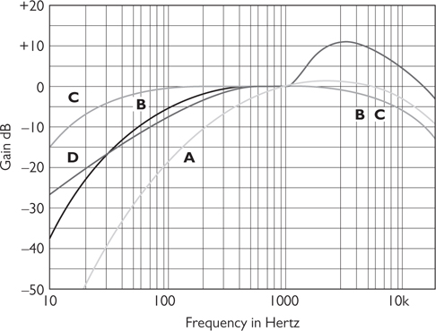
Figure 6-3    SPL weighting curves

The line marked “A” on this chart represents the A-weighted filter setting on an SPL meter. You can see that A-weighting discriminates against low-frequency energy. The A-weighting curve is almost the inverse of the equal loudness curve at a low listening level. The human ear perceives low-frequency energy as a lower dB SPL than it actually is. The energy is still there; it’s just that listeners are not as sensitive to it at these levels.

The A-weighting, therefore, is useful in low-listening-level situations, roughly 20 to 55 dB SPL. It lowers the dB SPL reading of low-frequency sounds to reflect how a human being perceives those sounds.

As the listening level increases to the 85 to 140 dB SPL range, the human ear response “flattens out.” You may then choose a C-weighted filter (indicated by the line marked “C” in Figure 6-3), whose curve is far less steep.

Loudness vs. Weighting

Figure 6-4 shows a side-by-side comparison of an equal loudness curve on the left and a weighting curve on the right. The equal loudness curve is a measure of sound pressure over the frequency spectrum of human hearing. It is an absolute value, using 0 dB SPL as a reference. The weighting curve represents standard filter contours used to make test instruments approximate the human ear. Therefore, the different weighting curves are meant to represent what the ear hears at various intensity levels. These measurements are a relative value and depend on where or what you are referencing for your measurement.

Figure 6-4    Equal loudness curves (left) and SPL weighting curves (right)

SPL Meter Weighting: Spectrum Analysis

Let’s take a look at two spectrum-analyzer readings taken from the same room. The first reading, shown in Figure 6-5 and fairly flat, was taken with no weighting applied. Notice that the overall dB SPL reading is 70.

Figure 6-5    Unfiltered audio signal on a spectrum analyzer

The second reading, shown in Figure 6-6, was taken using an A-weighted filter. The overall level, especially the low-frequency energy, is shown as reduced; now the meter reads 53.6 dB SPL. This reading reflects how a listener would actually perceive the noise in the room.

Figure 6-6    Audio signal on a spectrum analyzer with an A-weighted filter

Loudspeaker Directivity

A distributed loudspeaker system employs multiple loudspeakers that are separated from each other by some distance. This is most usually accomplished by installing the speakers in the ceiling above an audience area.

To design a distributed layout, you first must know how much area the sound from each of your selected loudspeakers will cover. For starters, use the polar-pattern directivity information provided by the loudspeaker manufacturer to create an elevation section view of a loudspeaker and the pattern. This will allow you to create a circular area that each unit will cover.

Loudspeaker coverage patterns are frequency dependent. This means that the exact pattern of coverage will depend on frequency. In other words, a loudspeaker rated a 90-by-40-degree loudspeaker covers only 90 by 40 degrees at a certain frequency. Remember that each frequency has a physical wavelength associated with it. A loudspeaker does not have the same coverage pattern across the entire audible frequency range.

Balloon plots are typically part of a loudspeaker’s specifications and are often available in computer files for use in various modeling programs, such as EASE. Computer modeling is commonplace (and necessary) in all but the simplest installations.

Figure 6-7 shows some of the plots from an EAW JF60 loudspeaker. Each concentric circle on these charts represents a change of 5 dB SPL. A polar pattern shows how far off-axis a loudspeaker’s coverage pattern extends at a given frequency. You can see that at high frequencies this loudspeaker’s energy drops off steeply as you move off-axis. As you move off-axis, look for the point at which the range of frequencies you’re using drops off by 6 dB SPL. The “6 dB down” point is typical for defining a loudspeaker’s coverage pattern.

Figure 6-7    Polar plots of different frequency bands for a loudspeaker

The specification sheet for this loudspeaker says its “nominal beam width” (coverage pattern) is 100 degrees horizontal by 100 degrees vertical. The axial grids are 5 dB divisions. Notice that the coverage pattern (dispersion) at 2 kHz is about 100 degrees wide. In other words, when comparing the level on-axis with the level 50 degrees off-axis, you should find a reduction in level of about 6 dB at 2 kHz.

The pattern shown at 125 Hz disperses in an omnidirectional pattern. Does this mean that low frequencies are omnidirectional? Not at all. It has to do with wavelength. It takes a larger device to control the dispersion pattern associated with the longer wavelengths of lower frequencies.

Realistically, the pattern shown for 2,000 Hz is the only one of these three that comes close to being 100 degrees by 100 degrees.

Calculating Loudspeaker Coverage

To create a loudspeaker layout, you must first determine two things: loudspeaker coverage angle and listener ear level.

By referencing the polar pattern information, you find the angle at which your highest target frequency is 6 dB below the on-axis level. For example, this might be at 40 degrees off-axis, which would provide a full 80 degrees of coverage for that target frequency.

Next, you must determine the listening ear height—the highest level being of most interest. For example, if you are designing a multipurpose room where the audience may be standing for some presentations and seated for others, design for the standing audience. The size of a loudspeaker coverage circle can be dramatically different when you factor in a low ceiling and a standing audience versus a higher ceiling and a seated audience, even with the same loudspeaker. See Figure 6-8 to help visualize your loudspeaker coverage calculation.

Figure 6-8    Calculating loudspeaker coverage

The formula for calculating the diameter (twice the radius) of the circle that represents the coverage area of a loudspeaker is as follows:

D = 2 * (H – h) * tan (C∠ / 2)

where:

•  D is the diameter of the coverage area.

•  H is the ceiling height.

•  h is the height of the listeners’ ears.

•  C∠ is the loudspeaker’s angle of coverage in degrees.

For example, if your loudspeaker provides 80-degree coverage, your ceiling height is 12 feet, and the audience is seated with an ear level of 4 feet, the following would give you your coverage area:

D = 2 * (H − h) * tan (C∠ / 2)

D = 2 * (12 − 4) * tan (80/2)

D = 2 * (8) * tan 40

D = 16 * 0.839

D = 13.4 feet, or a radius of 6.7 feet

In metric, if your ceiling height is 3.7 meters and your seated audience has an ear level of 1.2 meters, the following would give you your coverage area:

D = 2 * (H − h) * tan (C∠ / 2)

D = 2 * (3.7 − 1.2) * tan (80/2)

D = 2 * (2.5) * tan 40

D = 5 * 0.839

D = 4.2 meters, or a radius of 2.1 meters

Distributed Layout Options

When distributing loudspeakers, the goal is to place them in a strategic pattern to create a uniform sound source. You might design a distributed loudspeaker system when it’s not possible to implement a point-source system. For example, a certain ceiling height may be inadequate for a centralized, point-source speaker system because all listeners don’t have a good line of hearing to a central speaker or cluster.

You can use a number of patterns for a distributed loudspeaker system. As the amount of background noise in a space increases or the reverberation becomes high, loudspeaker pattern control becomes very important. Ultimately, the pattern you choose may be a compromise between the ideal and the attainable. Often, the available space for loudspeakers—or the budget—is less than desirable.

Uniformity of coverage is the greatest difference between distributed loudspeaker patterns. Generally, the more dense the pattern, the more uniform the coverage will be, but density will increase interaction among loudspeakers.

Designers should strive to minimize coverage where it’s not needed or where it can create problems. For example, you shouldn’t place loudspeakers where the audio will strike a wall before reaching listeners’ ears. This can cause uneven frequency response and phase cancellation at the listener position. Too much sound at the head of a conference table can cause feedback, so designers should make sure to implement a way to reduce levels or turn off offending loudspeakers in that area—or don’t put them there in the first place.

Figure 6-9 shows six common arrangements for distributed ceiling systems.

Figure 6-9    Six common coverage configurations for distributed loudspeakers

Edge-to-Edge Coverage

Edge-to-edge coverage places the loudspeakers in such a way that the furthest extent of their acoustic energy comes together at listeners’ ear level. There is no overlap with edge-to-edge patterns and therefore significant gaps. One loudspeaker’s coverage area is simply adjacent to the next; therefore, the distance between loudspeakers in this layout is two times the radius of the loudspeaker’s coverage pattern: (D = 2 * r).

This approach is inexpensive and results in minimum interaction between loudspeakers within a room. But an edge-to-edge configuration may result in an uneven SPL with low spots in the corners of the coverage area. This is least favorable in a business communication setting but may be appropriate for general paging or simple background music.

Maximum to minimum coverage variations for this configuration are around 4.35 dB. When deployed in a hexagon edge-to-edge pattern, coverage variations are around 5.4 dB.

Partial Overlap Coverage

Coverage patterns with minimal or partial overlap are among the most common methods of laying out distributed loudspeakers. In partial overlap systems, each loudspeaker’s coverage pattern overlaps about 20 percent of the adjoining speaker’s coverage pattern. Specifically, the minimum overlap in a square layout should be the radius of the loudspeaker polar pattern, multiplied by the square root of 2: (D = r * 1.4). In a hexagonal layout, that distance is the radius of the loudspeaker polar pattern, multipled by the square root of 3: (D = r * 1.7).

Partial overlap provides good coverage at most frequencies, with 3 dB of variation, and ensures few or no “low” spots. However, this approach may not produce a perfectly even frequency response because dispersion patterns vary according to the frequency of the sound. In addition, partial overlap may also create some negative interaction between nearby loudspeakers.

Edge-to-Center Coverage

An edge-to-center layout, or 50 percent overlap, will provide excellent coverage at most frequencies (with 1.4 dB variation). However, this is a costly approach because it requires many loudspeakers and will likely provide more coverage than required. Additional power amplification may also be required, plus additional installation labor.

Such a large amount of pattern overlap may also result in some negative interaction with the sound from nearby loudspeakers, such as uneven frequency response. This is because a dense overlap pattern may create too much pattern overlap within the space. Adding additional acoustic energy into a space can also reduce intelligibility, which will make it difficult for listeners to understand presenters.

In 50 percent overlap systems, each loudspeaker’s coverage pattern overlaps half of the adjoining coverage pattern, which can provide even SPL coverage. Whether using a square or hexagonal layout, the spacing distance between loudspeakers in a 50 percent overlap system equals the radius of the coverage circle: (D = r).

Ohm’s Law Revisited

In the audiovisual industry, Ohm’s law and the power equation are used to calculate and predict four properties of an electrical circuit: voltage, current, resistance, and power. They can help calculate the amount of current required to power the AV equipment within a rack or determine signal level at the end of a long cable run.

Ohm’s law defines the electrical relationships in direct current (DC) circuits. It can also help approximate for alternating current (AC) circuits. AC circuit calculations are frequency dependent, and Ohm’s law does not account for the influence of frequency in a circuit.

The results of Ohm’s law or power equation calculations can be given to a professional electrician or an AV systems designer to incorporate into a design. Before we go further in our discussion of loudspeakers, you may want to review Ohm’s law in Chapter 2.

Loudspeaker Impedance

Ohm’s law helps AV professionals calculate the total electrical impedance of a group of loudspeakers that are connected by cabling. Impedance is the opposition to the flow of electrons in an AC circuit. Like a DC circuit, an AC circuit contains resistance, but it also includes forces that oppose changes in current (inductive reactance) and voltage (capacitive reactance). Impedance takes into account all three of these factors.

Impedance is frequency-dependent, measured in ohms, and symbolized by the letter Z. If you know how to calculate voltage, current, and resistance using Ohm’s law, you can determine the impedance of loudspeakers as you’re setting them up and wiring them together.

On the back of almost any loudspeaker, you will see a nominal impedance rating. It is an important specification for loudspeakers, power amplifiers, and the inputs and outputs of equipment. Most common loudspeakers have a nominal impedance rating of 4, 8, or even 16 ohms. You may even see some that have an impedance of 6 ohms.

Audio signals are AC waveforms; therefore, you express audio signals in terms of frequency (cycles per second). Because impedance in an AC circuit is frequency-dependent, as frequency changes, so does the impedance of the circuit.

You will need to determine the resulting impedance of the loudspeaker line as you’re connecting and wiring together the loudspeakers.

Wiring Loudspeakers

Before installing loudspeakers, one of your first tasks is to verify the expected impedance of the loudspeaker-system circuit. If you don’t, you risk damaging equipment, personal injury, or simply poor system performance.

Ideally, you can complete this step before leaving for the jobsite. But sometimes, circumstances require you to make calculations in the field. If the expected impedance is not indicated on drawings or documentation, then you need to come up with it yourself. The formula you use depends on how the loudspeakers will be wired: in a series, in parallel, or a combination of the two. Let’s examine each scenario.

Loudspeakers Wired in a Series

When loudspeakers are wired in a series, each loudspeaker’s coil is connected to the next loudspeaker in the series, in sequence. The power amplifier’s positive output terminal connects to the positive terminal of the first loudspeaker. The first loudspeaker’s negative terminal connects to the second loudspeaker’s positive terminal. The second loudspeaker’s negative terminal connects to the third loudspeaker’s positive terminal, and so on. The last loudspeaker’s negative terminal completes the circuit by connecting to the amplifier’s negative terminal.

The formula for calculating the total impedance of a series loudspeaker circuit is as follows:

Z_T = Z₁ + Z₂ + Z₃+ …Z_N

where:

•  Z_T is the total impedance of the loudspeaker circuit.

•  Z_N is the impedance of each loudspeaker.

Figure 6-10 shows three loudspeakers wired in series—plus to minus to plus to minus. If you want to calculate the total impedance of this loudspeaker circuit, you would simply add the impedances of the individual loudspeakers.

Figure 6-10    Speakers wired in a series

If each of these loudspeakers has a nominal impedance of 8 ohms, the total impedance is 24 ohms.

Loudspeakers Wired in Parallel, Same Impedance

Another method of connecting loudspeakers in a circuit is to wire them in parallel. This means that the positive output of the amplifier connects to every loudspeaker’s positive terminal, and each loudspeaker’s negative terminal connects to the amplifier’s negative terminal.

Loudspeakers wired in parallel can have the same or different impedances. The formula for finding the circuit impedance for loudspeakers wired in parallel with the same impedance is as follows:

Z_T = Z₁ / N

where:

•  Z_T is the total impedance of the loudspeaker system.

•  Z₁ is the impedance of one loudspeaker.

•  N is the quantity of loudspeakers in the circuit.

Figure 6-11 shows three loudspeakers wired in parallel. If all the loudspeakers have the same impedance, the impedance of the loudspeaker divided by the number of loudspeakers wired in parallel equals the impedance of the circuit. If you have three loudspeakers wired in parallel, each rated at 8 ohms, the circuit’s impedance is 2.67 ohms (8 ohms/3).

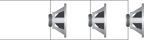
Figure 6-11    Speakers wired in parallel

Loudspeakers Wired in Parallel, Different Impedances

If loudspeakers wired in parallel have different impedances, you must use a different formula for finding the total impedance of the circuit. The formula for finding the circuit impedance for loudspeakers wired in parallel with differing impedance is as follows:

where:

•  Z_T is the total impedance of the loudspeaker circuit.

•  Z_1-N is the impedance of each individual loudspeaker.

If you have three loudspeakers wired in parallel, with the first rated at 4 ohms, the second rated at 8 ohms, and the third rated at 16 ohms, the circuit’s impedance is 2.29 ohms, or Z_T = 1/((1/4 ohms)+(1/8 ohms)+(1/16 ohms)).

Loudspeakers Wired in a Series and Parallel Combination

In a series/parallel loudspeaker circuit, groups of loudspeakers, called branches, are wired together in series. Typically, loudspeakers in the same branch have the same impedance. Each branch is connected to the positive and negative lines of the amplifier in parallel.

To calculate the total impedance of a series/parallel circuit, you must do the following:

•  Calculate the total impedance of each branch using the series circuit impedance formula, as described earlier.

•  Calculate the total circuit impedance of the circuit using the parallel circuit impedance formula, as described earlier.

Measuring Impedance

Before electrically testing the loudspeaker circuit, refer to your impedance calculations and compare it to readings from an impedance meter. An impedance meter is a piece of test equipment used to measure the true impedance in an entire loudspeaker or loudspeaker circuit. Most are portable and battery operated, similar to a multimeter.

When working with large systems, check the line impedance often. Do not wait until all the loudspeakers are wired to find out that one is bad. As you install a group of loudspeakers, test it to make sure there are no problems before you install the next group. Be sure to write down the final measured impedance. This final measurement will be useful for future system service and maintenance.

Moreover, always check the system load prior to connecting the loudspeakers to an amplifier. Too little impedance on the output of the amplifier will cause the amplifier to drive too much current into the loudspeakers and may cause the amplifier to fail.

To measure impedance, take the following steps:

1. Disconnect the wires from the amplifier.

2. Calibrate the meter by doing the following (analog meters only):

a. Connecting the test leads to the meter

b. Using the three range buttons and selecting the scale that is appropriate for your expected value for greatest accuracy

c. Holding the test leads together so the tips are touching, or pressing and holding the “zeroing” button

d. Rotating the calibration knob until the reading indicates 0

3. Connect one lead to each of the wires on the first loudspeaker in the chain. Polarity is not important.

4. Observe the reading and compare it with the expected reading. It should be within a certain tolerance; otherwise, there may be problems.

5. Reconnect the loudspeaker wires and power on the amplifier.

Transformers

Voltage can be manipulated in an electrical circuit by using transformers. Transformers are common electrical devices that are used in power supplies, audio/video circuits, and loudspeaker systems.

Transformers work by placing two coils against each other, usually wound around a common piece of iron. A coil may also be known as a winding. Basic physics explains that alternating current, such as audio signals, flowing through a coil will create a magnetic field.

The input coil is often referred to as the primary winding, and the output coil is the secondary winding.

The current is transferred by electromagnetic induction, a process that transfers a current from an input to an output coil. This means that the current from the source, flowing through the first coil, creates a magnetic field.

Because the two coils in electromagnetic induction are not physically connected to each other, the input and output are “isolated” from each other. This is where the term isolation transformer comes from.

Transformers can increase or decrease the voltage in a circuit; they can also keep it the same. If the ratio of turns in the input and output coils are 1 to 1, the voltage output will be the same as the input, minus what is known as insertion loss.

You can use a 1:1 isolation transformer (Figure 6-12) to isolate one circuit (audio or video) from another to solve a ground loop problem, such as an audio hum or rolling lines in a video image.

Figure 6-12    A 1:1 transformer

If the ratio of turns in the input and output coils are 1 to 2, the voltage output will be doubled. This is known as a step-up transformer. A 1:2 step-up transformer (see Figure 6-13) has twice as many windings on the secondary side as it does on the primary side. With twice as many windings, twice as much voltage will be induced into the secondary side. In other words, the magnetic lines of force (flux) from the conductors on the primary side will cut across twice as many conductors on the secondary side. This means that the voltage will be induced across twice as many conductors as compared to the primary side.

Figure 6-13    A 1:2 step-up transformer

If the ratio of turns in the input and output coils are 2 to 1, the voltage output will be lowered by 1/2. This is known as a step-down transformer.

A 2:1 step-down transformer (see Figure 6-14) has half as many windings on the secondary side as opposed to the number of windings on the primary side. Even though the voltage will be carried on half as many windings, the power will be equal on both sides, minus a small amount of insertion loss. Instead, either the voltage will increase or the current will decrease.

Figure 6-14    A 2:1 step-down transformer

Specifying a Power Amplifier

Once loudspeaker locations have been determined, the next step is to calculate how much power is needed at the loudspeaker to provide adequate SPL at the listener location. This calculation would also include the necessary headroom appropriate to the application. Headroom is the difference in dB SPL between the peak and average-level performance of an audio system. For a speech application, the recommended value is 10 dB; for program audio, it’s as much as 20 dB.

To determine the power required at the loudspeaker, you need to know the following:

•  The sound pressure level required from the sound system at the listener position. For speech applications, this is typically 70 dB SPL.

•  The headroom required. For speech applications, 10 dB is considered adequate. For music applications, as much as 20 dB or more may be required.

•  Loudspeaker sensitivity. Typically this will be stated as SPL in decibels expected at a distance of 1 meter away from the loudspeaker with 1 watt applied.

•  Distance to the farthest listener from the loudspeaker.

Once you have this information, you can calculate the amount of power needed at the loudspeaker, also known as the electrical power required (EPR), or wattage at the loudspeaker. You calculate EPR using this formula:

where:

•  EPR is the amount of electrical power required at the loudspeaker.

•  L_P is the SPL required at distance D₂.

•  H is the headroom required.

•  L_S is the loudspeaker sensitivity reference, usually 3.28 feet (1 m).

•  D₂ is the distance from the loudspeaker to the farthest listener.

•  D_r is the distance reference value.

•  W_ref is the wattage reference value; assume a W_ref of 1, unless otherwise noted.

Headroom Requirements

A sound reinforcement system needs to be loud enough for the listeners to hear it. When choosing a loudspeaker, you must verify that the loudspeaker is sensitive enough to boost the sound signal with enough headroom.

System headroom is the difference between the audio system’s typical operation level and the maximum level the system can attain. If a sound system usually operates at +1 dBV but could operate as high as +20 dBV, then it has 19 dB of headroom. It is important to have enough headroom to handle momentary performance boosts.

As noted earlier, for a speech-only sound reinforcement system, 10 dB of headroom is appropriate. For a music reinforcement system, as much as 20 dB of headroom is needed to avoid clipping musical peaks.

Loudspeaker Sensitivity

Like microphones, loudspeakers are rated based on their ability to convert one energy form into another. This rating is called a sensitivity specification, and it defines the loudspeaker’s acoustic output signal level, given a reference input level. Put another way, sensitivity defines how efficiently a loudspeaker transduces—or converts—electrical energy into acoustic energy.

Given the same reference electrical input level into two different loudspeakers, a more sensitive loudspeaker would provide a higher acoustical energy output than a less sensitive loudspeaker.

Loudspeakers vary quite a bit when it comes to efficiency. Does this mean that lower-sensitivity loudspeakers are of lesser quality? Not at all. Like microphones, loudspeakers are designed and chosen to meet specific uses.

Power Amplifiers

Now that you know how many watts are needed at the listener position, you can specify the power amplifier. A power amplifier boosts the audio signal enough to move the loudspeakers.

Power amplifiers are designed to be connected to a specific load (impedance)—either a low-impedance load (typically 2 to 8 ohms) or a high-impedance load, such as with a distributed or constant-voltage loudspeaker system. The power amplifier’s specifications should tell you what kind of impedance load it can be connected to. Some power amplifiers have a switch that allows them to connect to various impedance loads. Other power amplifiers may require an internal or external transformer to function with a 70 V or 100 V load.

Specifying a Power Amplifier for Direct-Connection Audio

To specify a power amplifier for direct connection audio, follow these steps:

1. Determine the SPL at the listener position.

2. Add 10 dB for voice or 20 dB for music.

3. Find the loss over distance in dB by taking the 20log of the dB-SPL at the listener position (D₂) divided by the loudspeaker’s sensitivity in dB-SPL (D_r). Written another way, this is 20log(D₂/D_r).

4. Determine the power (watts) required at the loudspeaker using the EPR formula.

5. Round the result up to an amplifier value that can be readily purchased.

Specifying a Power Amplifier for Distributed Audio

This is a process for specifying a power amplifier for a distributed audio system. In this type of audio system, you need to specify your tap settings before you can determine your amplifier need.

1. Determine SPL at the listener position.

2. Add 10 dB for voice or 20 dB for music.

3. Find the loss over distance in dB by taking the 20log of the dB-SPL at the listener position (D₂) divided by the loudspeaker’s sensitivity in dB-SPL (D_r). Written another way, this is 20log(D₂/D_r).

4. Determine the power (watts) required at the loudspeaker using the EPR formula.

5. Select the appropriate tap value for the loudspeaker based on watts required.

6. Repeat steps 1–5 for each loudspeaker.

7. Sum the tap settings from all loudspeakers.

8. Increase the total tap settings by a factor of 1.5.

9. Round the result up to an amplifier value that can be readily purchased.

Microphones

If you’re designing an audio system, chances are it will include microphones. Clients use microphones to be heard—in presentations, conferences, or performances. In this section, you will learn about the special qualities of microphones and how they factor into AV systems. We’ll start by discussing the different types of microphones you might specify in a design.

Handheld Microphones

Handheld microphones are used mainly for speech or singing. Because they’re constantly moving, handheld microphones include internal shock-mounting to reduce handling noise. Handheld microphones can be held in the hand or mounted on a lectern or stand for hands-free operation.

Instrument, Lavalier, and Head Microphones

Lavalier and head microphones are worn by users. A lavalier (also called a lav or lapel microphone) is attached directly to clothing, such as a necktie or lapel (pictured in the following illustration).

A head microphone (also called a headmic), is a microphone that is attached to a small, thin boom and fitted around the ear (on the right).

Because size, appearance, and color are key considerations for these types of microphones, lavaliers and headmics are often electret microphones, a type of condenser microphone that can be powered with small batteries. We will discuss electret microphones later in this chapter. Lavaliers and head mics are usually worn by presenters and commonly used in television and theater productions.

Boundary and Gooseneck Microphones

Boundary microphones (sometimes known as pressure-zone microphones [PZMs]) are mounted directly against a hard surface, such as a conference table, wall, or ceiling. They rely on reflected sound from the surrounding surface and are also called surface-mount microphones. Keep in mind that the acoustically reflective properties of the mounting surface affect the microphones’ performance.

Although they can be much less obtrusive in a conference table than a gooseneck mic, boundary microphones may be subject to papers accidently being placed over them, laptop fans blowing on them, and more.

Mounting a microphone on a ceiling typically yields the poorest performance because the sound source is much farther away from the intended source and much closer to other noise sources, such as ceiling-mounted projectors, heating, ventilation, and air conditioning (HVAC) diffusers, and other devices.

Gooseneck microphones (as seen in the following illustration) are often used on lecterns and conference tables. Such microphones are attached to flexible or bendable stems, which come in varying lengths.

Shock mounts are available to isolate the microphone from table or lectern vibrations.

On a conference table, although goosenecks generally get the microphone closer to the source than a boundary microphone, they can create an undesirable appearance in the space or, in the case of videoconferencing, on camera. (Picture what’s sometimes called a gooseneck farm.)

Shotgun Microphones

Shotgun microphones are named for their physical shape, as well as their long and narrow polar pattern. A shotgun microphone is a long, cylindrical, highly sensitive, unidirectional microphone used to pick up sound from a great distance.

Most often used in film, television, and field production work, a shotgun microphone can be attached to a long pole called a fish pole or studio boom. The boom is often used by a boom operator (as seen in the following illustration) or fitted to the top of a camera.

Microphone Construction

Microphones come in two main versions, based on construction: dynamic and condenser. A dynamic microphone is a pressure-sensitive microphone with a moving-coil design that transduces sound into electricity using electromagnetic principles.

Dynamic microphones are economical, durable, and capable of handling high sound pressure levels. Unlike condenser microphones, they don’t require a source of power, often called phantom power.

Condenser microphones transduce sound into electricity using electrostatic principles. Condenser microphones are generally sensitive, which means you’ll get more electrical signal and higher sound quality from a condenser microphone than from a dynamic microphone. They are excellent for boardrooms or classrooms where you need to pick up quieter signals, such as a person talking.

Condensers aren’t as durable as dynamic microphones, however, and they do require phantom power.

Microphone Polar Response

One of the characteristics to consider when selecting a microphone is its polar response or pickup pattern. The pickup pattern describes the microphone’s directional capabilities—its ability to pick up the desired sound from a certain direction while rejecting unwanted sounds from other directions.

Pickup patterns are defined by the directions in which the microphone is most sensitive. These patterns help you determine which microphone type to use for a given purpose.

There will be occasions when you want a microphone to pick up sound from all directions (such as an interview), and there will be occasions when you do not want a microphone to pick up sounds from nearby sources surrounding it (such as people talking or papers rustling). The pickup pattern is also known as the polar pattern, or the microphone’s directionality.

Different types of pickup patterns include the following:

•  Omnidirectional    Sound pickup is uniform in all directions.

•  Cardioid (unidirectional)    Pickup is from the front of the microphone only (one direction) in a cardioid pattern. It rejects sounds coming from the side but mostly rejects sound from the rear of the microphone. The term cardioid refers to the heart-shaped polar plot.

•  Hypercardioid    A variant of cardioid. It’s more directional than a regular cardioid mic because it rejects more sound from the sides. The trade-off is that it will pick up some sound from directly behind the microphone.

•  Supercardioid    Provides better directionality than hypercardioid, with less rear pickup.

•  Bidirectional    Pickup is equal in opposite directions with little or no pickup from the sides. This is sometimes also referred to as a figure-eight pattern, referring to the shape of its polar plot.

Polar Plot

The polar plot is a graphical representation of a microphone’s directionality and electrical response characteristics (see Figure 6-15).

Figure 6-15    Polar plots of one microphone at 125 Hz, 2 kHz, and 8 kHz

Although a frequency-response graph shows the level of decibels at a given frequency, the polar plot shows the level of decibels by angle, or the pickup pattern of the microphone. Typically, microphone specifications will include several polar plots, each showing the pickup pattern at a different frequency.

Imagine a microphone in the center of the plot, pointing straight at 0 degrees. If you stood at the 0-degree point, you’d be standing right in front of the microphone. At the 180-degree point on the plot, you would be directly behind the microphone.

The polar plot shows the angles from which the microphone picks up and transduces sound at the highest voltage. It extends farthest toward the 0-degree point, which shows that the microphone is best at detecting sounds coming from directly in front of it. To the left and right of the 0-degree mark, the curve falls away. This means as you move farther to the left or right of this microphone, it “hears” you a little less well. In Figure 6-15, the microphone picks up no sound at all from directly behind at 2 kHz, though it picks up some sound from behind at 125 Hz and 8 kHz.

Polar plots help you select and position a microphone. For example, say you need a microphone to pick up audio in a conference room. You want people on all sides of the table to be heard, so you would choose a mic whose polar pattern displays even pickup in all directions in the frequency range of the human voice.

Microphone Frequency Response

The frequency-response specification is an important measure of a microphone’s performance. It defines the microphone’s electrical output level over the audible frequency spectrum, which in turn helps to determine how a microphone “sounds.”

Frequency response is a way of expressing a device’s amplitude response versus frequency characteristic, as shown in Figure 6-16. A frequency response is usually presented as a graph or plot of a device’s output on the vertical axis versus the frequency on the horizontal axis.

Figure 6-16    Microphone frequency response

A microphone’s frequency response gives the range of frequencies, from lowest to highest, that the microphone can transduce. It is often shown as a plot on a two-dimensional frequency response graph. A microphone’s frequency response graph shows the voltage of its output signal relative to the frequency of the sounds it picks up.

With directional microphones, the overall frequency response will be best directly into the front of the microphone. As you move off-axis from the front of the microphone, not only will the sound be reduced, but the frequency response will change.

Microphone Signal Levels

A microphone, regardless of the type, produces a signal level called mic level. Mic level is a low-level signal—only a few millivolts (abbreviated as mV to express one-thousandth of a volt). Table 6-2 shows the relative voltages of different signal levels.

Table 6-2    Comparing Signal Levels

Because mic level operates at only a few millivolts, it is prone to interference. A microphone preamplifier amplifies the mic level signal to line level for routing and processing. Line level is the strength of a regular audio signal and is used for all routing and processing between components. In a professional audio system, line level is about 1.23 volts (+4 dBu); consumer line level is 0.316 V (−10 dBV). When you see an RCA or phono connector, it often indicates a consumer-level signal.

Once the audio system has routed and processed the signal, it is sent to the power amplifier for final amplification up to loudspeaker level. The loudspeaker takes that amplified electrical signal and transduces the electrical energy into acoustical energy (see Figure 6-17).

Figure 6-17    Mic level to line level to loudspeaker level

Microphone Sensitivity

Another important performance criterion that characterizes a microphone is its sensitivity specification. Sensitivity defines how efficiently a microphone converts acoustic energy into electrical energy. It is expressed as decibels of voltage per pascal of sound pressure (dBV/PA).

For example, a microphone may have a sensitivity specification that reads as follows: −54.5 dBV/PA (1.85 mV) 1 Pa = 94 dB SPL. This means that with a reference level of 94 dB SPL into the microphone, it will produce a voltage level of −54.5 dBV (0.00185 V) out.

One pascal is equal to 94 dB SPL. If a microphone with the previous specification receives less than 94 decibels of sound pressure, it will output less than −54.5 dBV. Less acoustical energy in will result in less electrical energy out.

If you expose two different microphones to an identical sound input level, a more sensitive microphone provides a higher electrical output than a less sensitive microphone. Condenser microphones are usually more sensitive than dynamic microphones.

Does this mean that lower-sensitivity microphones mean lesser quality? Not at all. Microphones are designed and chosen for specific uses. A professional singer using a microphone up close can produce a high SPL. In contrast, a presenter speaking behind a lectern and a foot or two away from the microphone produces much less sound pressure. The singer needs a less sensitive microphone than the person talking.

For the singer, a dynamic microphone may be the best choice because it will typically handle the higher SPL produced by the singer without distortion while still providing more than adequate electrical output. The presenter would benefit from a more sensitive microphone, such as a condenser mic.

When determining microphone sensitivity, you will need to consider three factors.

•  Sound pressure level    The acoustic energy is at the microphone.

•  Electrical signal level    The goal is to have a line-level signal after the preamplification.

•  Matching levels    Can the signal level from the microphone/preamp combination be amplified to the line-level signal that the audio system (mixer) requires?

Microphone Pre-Amp Gain

Let’s say you need to choose a microphone for a new auditorium. Your sound source is a presenter located 2 feet (609.6 mm) away from the microphone, with a measured SPL of 72 dB. To route and process that signal, you need to amplify the microphone-level signal to line level (0 dBu). Most microphone preamplifiers will provide around 60 dB of amplification.

You have a choice between two microphones (remember, 1 Pascal = 94 dB SPL).

•  Dynamic Microphone A, with an equivalent voltage specification of −54.5 dBV/Pa (1.85 mV)

•  Condenser Microphone B, with an equivalent voltage specification of −35.0 dBV/Pa (17.8 mV)

In this scenario, your microphone specification sheets tell you that if you put 94 dB SPL into each microphone, –54.5 dBV and −35.0 dBV will be produced, respectively. You need to select a microphone that will provide an adequate signal level for the application. To do this, you need to know what the required microphone pre-amp gain is for each microphone. Refer to Figure 6-18 for the formula.

Figure 6-18    Microphone pre-amp gain formula

To calculate the pre-amp gain for your microphones, follow these steps:

1. Determine the level (in dB SPL) that is measured with an SPL meter at the microphone position. Record this at position 1.

2. Determine your microphone reference level (dB SPL). You will find this number on your microphone specification sheets. Record this at position 2.

3. Determine the microphone sensitivity value (dBV). This is the negative number indicated on the specification sheet. Record this at position 3.

4. Convert the dBV value from step 3 to dBu. The formula for this is 20log(dBu/dBV) = 20log(1/0.77) = 2.2 d. Record this value at position 4.

5. Record the output level required at position 5. This is generally 0 dBu or +4 dBu.

6. Now do the match: The pre-amp gain required is position 1 – 2 + 3 + 4 – 5.

In this example, the pre-amp gain required for Dynamic Microphone A is −74.29 dBu. The pre-amp gain required for Condenser Microphone B is −54.79 dBu.

Assuming you have a 60 dB gain in your microphone pre-amp, Dynamic Microphone A is not sensitive enough for this application. The closer you can get to 0 dBu, the better the microphone will be for the application. You need 83.5 dB, but you have only 74.29 dB gain, leaving you 9.21 dB short.

Does this make Dynamic Microphone A a bad mic? No. It is designed for a different application—speaking or singing at a much closer range than 2 feet (610 mm) and with much more acoustic input. In this case, the mixer’s preamplifier would normally be more than adequate to amplify Dynamic Microphone A’s signal to line level.

With a pre-amp gain of −54.79 dBu, Condenser Microphone B is sensitive enough for this application. The combination of the more sensitive microphone and the gain available from the microphone preamplifier in the mixer can take the mic level signal to the 60 dBu level needed for signal routing and processing.

Microphone Mixing and Routing

Aside from microphones amplified to line level, your audio system will include other sources, originating at line level. For professional audio line sources, little, if any, amplification will be required for routing and processing. Consumer line level may require some amplification.

An automatic microphone mixer is meant to control the number of open microphones (NOM) to the loudspeaker. The user can set NOM on the mixer, but generally it’s limited to one. The following are some of the settings where using an auto mixer would be ideal:

•  Conference rooms

•  Courtrooms

•  Meeting spaces

•  Live events with handheld microphones

In these settings, you have multiple people speaking and need a way to control the different line sources. The big question is, “How many people need to talk at any one time?”

If there are multiple people who need to speak, you can assign a NOM that reflects that number. However, keep in mind that the number of open microphones affects the chances of feedback in the system. The fewer microphones open, the fewer chances of feedback or extraneous noise coming through the loudspeaker.

There are two ways an auto mixer can limit the NOM in a design: gated or gain sharing. With gated sharing, each channel is set to an adjustable sound threshold that a microphone needs to surpass to be turned on. If it falls below that threshold, it is muted. The threshold must be set high enough to keep the channel from being opened by background noise yet low enough to open when someone is speaking. This creates a binary effect—each microphone is either on or off. But there is a chance that the system can’t pick up the first-spoken syllables of a low talker if not set correctly and varying levels from conference participants (soft to loud) can lead to choppy audio.

With gain sharing, the available gain is shared among all of the channels, and microphones with more signal get more gain. (Those with less receive less.) Because all the microphones are splitting gain depending on activity, pick up is gradual, resulting in smoother operation and greater sophistication than a gated design.

Microphone Placement: A Conference Table

Let’s say you need to place microphones around a conference table. Here are two possible options:

•  Six cardioid mics—one microphone per every two participants, with one each for the participants at the ends of the table (see Figure 6-19).

•  Two omnidirectional mics (see Figure 6-20). Although two omnimicrophones would seem to cover the participants, you must also consider the environment. Omnidirectional mics are equally sensitive to sounds coming from all directions, so ask yourself, for example, “Will there be a projector above the table?” and “How loud will background noise from the HVAC system be?”

Figure 6-19    A conference table with a cardioid microphone coverage pattern

Figure 6-20    A conference table with an ominidirectional microphone coverage pattern

Microphone Placement: The 3:1 Rule

When using multiple microphones, consider how the sound from a presenter will reach the microphones.

In Figure 6-21, each person has been given their own microphone. When a presenter speaks, their voice is picked up by three microphones. The microphone directly in front picks up the sound louder than the off-axis microphones do. In addition, because they are farther away, the sound that these two microphones pick up may be out of phase.

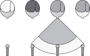
Figure 6-21    Each mic is 1 foot away from one presenter and 1 foot away from all other mics.

Let’s say the mics are separated by 1 foot and are 1 foot away from the person talking. The front mic picks up the talker at 65 dB SPL. What are the two mics picking up?

The outside mics are this far away:

C = √(12 + 12)

C = √(1 + 1)

C = √(2)

C = 1.41

The loss over distance is as follows:

dB = 20log(1.41/1)

dB = 2.98 or about 3 dB less (not very much)

In an analog mixer, the three microphones would be “mixed” together. The phase differences between the microphones create a comb-filter effect in the sound’s frequency response, which gives it a thin, hollow tone quality.

In Figure 6-22, the microphones are separated at a greater distance, this time at a ratio of 3:1. That is, the distance between each microphone is three times the distance between the microphone and a presenter.

Figure 6-22    Each mic is 3 feet away from each other and 1 foot away from one presenter.

By separating the microphones using the 3:1 rule, the outside microphones are this far away:

C = √(12 + 32)

C = √(1 + 9)

C = √(10)

C = 3.16

The loss over distance is as follows:

dB = 20log(3.16/1)

dD = 9.48 or about 10 dB less, which sounds half as loud

When the three microphones are mixed together in an analog mixer, the phase differences between the microphones will still affect the sound. However, the levels being mixed are greatly reduced because of the distance, which makes the comb filtering less noticeable.

Reinforcing a Presenter

If you need to mic only one specific person, you have a few options for reinforcing their voice.

Wireless lavalier microphones are effective for film or training presentations where the microphone needs to be “invisible.” The best position for a wireless lavaliere will be in the center of the chest, just below the hollow of the throat. You want to get the microphone as close to the presenter’s mouth as possible, but take care to avoid any positions that might cause unwanted contact.

An ear-worn microphone is another hidden microphone solution. Ear microphones should be placed about a quarter-inch (10 mm) away from the corner of the performer’s mouth. Do not position the element directly in front of the mouth because it will pick up “plosives” (Ps, Ds, and Ts) and breath sounds. Place the element so it does not directly contact or rub the cheek of the presenter.

If an ear microphone is not available, a lavalier placed along the center of the chest, as close as possible to the mouth, is best. Ask the presenter to tilt their chin down as low to the chest as they possibly can and place the microphone just below that point.

Handheld microphones will always give better gain before feedback when held as close to the mouth as possible. Advise presenters to hold the mic just below their chin.

Microphones and Clothing

When reinforcing (micing) a presenter, you need to consider the presenter’s clothing. Here are some examples:

•  If the presenter is wearing a suit, you may be able to hide the microphone inside the knot of a tie.

•  Avoid placing the microphone near silk. Silk blouses and ties can sound scratchy if they move against the microphone.

•  There are protective mounts that can be taped to the performer’s chest and prevent rustling noises from clothing.

•  If your project involves a wardrobe manager, working closely with that person may make microphone placement easier.

Polar Plots for Reinforcing a Presenter

When reinforcing a presenter with a lavalier microphone, you need to consider microphone placement and polar patterns. A lavalier microphone with a cardioid polar pattern will capture the presenter’s voice without capturing background noise from other directions (see Figure 6-23).

Figure 6-23    Proper placement of a cardioid lavalier microphone

This directional microphone is an excellent choice, but only if you know that the end users are all trained in how to place the microphone. For example, what if the user places the cardioid microphone off-center, on their lapel? What if they place the microphone upside down?

Instead of specifying a microphone with a cardioid polar pattern, consider specifying one with an omnidirectional polar pattern. An omnidirectional microphone will pick up the presenter’s voice, even if it is placed off-center or upside down (see Figure 6-24).

Figure 6-24    Proper placement of an omnidirectional lavalier microphone

Audio System Quality

Now that you’ve learned how humans perceive sound and how sound is measured, you need to ensure the quality of the audio system and how it functions in the space. For one thing, you need to determine whether the audio system will be stable by comparing a couple of calculations, namely, potential acoustic gain and needed acoustic gain. You also need to check your sound-reinforcement design to make sure it will be effective based on the client’s audio system needs.

Sound reinforcement is the combination of microphones, audio mixers, signal processors, power amplifiers, and loudspeakers that are used to electronically amplify and distribute sound.

To work properly, a sound system must accomplish three things.

•  It must be loud enough.

•  It must be intelligible.

•  It must remain stable.

Before we delve into PAG-NAG equations and a fundamental goal of audio system design—eliminating nasty feedback—let’s discuss further these three measures of audio system quality.

It Must Be Loud Enough

Can the listener hear the intended audio? If the answer is no, you have a problem. This may be a simple matter of changing the listener or loudspeaker location or increasing the volume. It may also be a sign of a much greater issue, such as unfriendly acoustics.

“Loud enough” depends on the application. Although sound systems encompass everything from conference rooms to rock ’n’ roll concerts, for now, at least, we’ll focus on the context of a typical boardroom, conference room, or lecture hall.

For each audio system, you need a target sound pressure level. For a typical speech reinforcement system, that level is around 60 to 65 dB SPL. That is the speech level of a human about 2 feet (0.6 meters) away. Through the audio system you’re designing, your goal is to replicate that conversational level with the audience. One key consideration in achieving this is the signal-to-noise (S/N) ratio and its effect on audio loudness.

Signal-to-noise ratio is the ratio, measured in decibels, between the audio (or video) signal and the noise accompanying the signal. In your design, look for an acoustic signal-to-noise (S/N) ratio of 25 dB. This means you should have 25 dB between the level of the sound system, your signal, and the level of the room’s background noise level.

Using a 25 dB S/N ratio, you can arrive at the required loudness of the audio system two different ways. First, imagine you’ve measured a background noise level of 55 dB SPL. Your system target level then needs to be 25 dB above that—80 dB SPL. But 80 dB SPL would be a loud level for conversation.

Coming at it from a different direction, start with your target. Say you want to achieve 65 dB SPL. Your background noise level should be 25 dB less than that—40 dB SPL. Think of this as the signal-to-noise level of the acoustic environment and design your acoustic space with that in mind.

It Must Be Intelligible

Intelligibility describes an audio system’s ability to produce a meaningful reproduction of sound. For example, an intelligible sound-reinforcement system can reproduce accurately the vowels and consonants of a source, which helps listeners identify words and sentence structure, giving the sound meaning.

In audio system design, intelligibility deals with the intensity and time arrival of the indirect sound. Reflected and reverberated sound energy arrives at the listener’s ear after direct sound, which comes directly from the loudspeaker. Late reflections sound like distinct echoes, and excessive reverberation masks intelligible speech.

Whether in amplified or unamplified speech presentation, the requirements of speech intelligibility are very much the same.

•  Speech loudness level    Average speech levels should be in the 60 to 65 dB range, if people with normal hearing are to understand it without effort. Under noisy conditions, the speech level should be raised accordingly.

•  Speech signal-to-noise ratio    For ease in listening, average speech levels should be at least 25 dB higher than the prevailing noise level. However, at elevated speech levels, in noisy environments, a somewhat lesser speech-to-noise ratio is possible. Typically, a 15 dB S/N ratio may suffice in situations where considerable noise is expected, such as live sports where there are spectators.

Normal face-to-face speech communication is about 60 to 65 dB SPL, but most speech reinforcement systems operate between 70 and 75 dB SPL. If the level of amplified speech increases beyond that range, to about 85 to 90 dB SPL, overall intelligibility won’t increase much, and most listeners will complain of excessive levels. Any louder, and intelligibility will diminish because listeners will feel oppressed by the high levels.

The direct-to-reflected sound ratio is a measure of the different energy in a space. It takes the level of direct sound—from source to listener—and compares it to the level of reflected sound, all of which arrives at the listener by an indirect pathway and determines the intelligibility.

Whether reflected sound is a problem or not comes down to two things.

•  How late did it arrive at the listener in relation to the direct sound?

•  At what energy level did that reflection arrive at the listener?

If the reflection arrives at the listener 50 to 80 milliseconds or later than the direct sound and at a sufficient energy level, it is considered an echo, and it adversely affects intelligibility.

It Must Remain Stable

Stability applies to audio systems that employ microphones in the same space. Can the client turn up the volume loud enough to be heard without causing feedback? If someone must make constant adjustments to eliminate feedback, chances are the system wasn’t designed properly.

To determine whether an audio system is stable, a designer calculates gain before feedback—how loud the loudspeakers get before the microphones pick them up. Gain before feedback is frequently referred to as potential acoustic gain, which you will learn about later in this chapter.

Gain before feedback is largely a design issue. It has to do with distance relationships between the source (such as a presenter) and the microphone, the microphone and the loudspeakers, and the loudspeakers and the listeners.

The designer must also determine the amount of gain—or amplification—required from the audio system to produce an adequate sound level. How loud do the loudspeakers need to be for listeners to hear the intended audio? This is known as needed acoustic gain, which you will also learn about later.

By comparing PAG to NAG, you can determine whether a system will be stable. If the system exhibits more potential acoustic gain than needed acoustic gain, it will be stable. But if its needs exceed its potential, either the client won’t be able to turn the volume up loud enough or feedback may occur.

PAG/NAG

As you learned earlier, the quality of an audio system can be summed up by three easily understood concepts: Is the audio loud enough? Can the audio be understood? Does the audio system operate in a stable manner?

To reiterate, audio system stability refers to the system’s ability to amplify sound from a microphone without feedback or distortion. Proper equipment selection and placement are significant contributors to system stability (think acoustic treatment, equalization, feedback suppression, and mix-minus), but controlling acoustic gain is also an important method. A sufficient PAG/NAG ratio will minimize the potential for feedback.

NAG is the gain the audio system requires to achieve an equivalent acoustic level at the farthest listener equal to what the nearest listener would hear without sound reinforcement. It tells the designer how much you need to increase the amplitude of a sound wave on a microphone for it to be equivalent to some closer location, where no amplification would be required. Again, NAG is relevant only for systems incorporating microphones that are being reinforced in the same space.

Before you can solve for NAG, you need to understand equivalent acoustic distance (EAD). EAD is the farthest distance one can go from the source without needing sound amplification or reinforcement to maintain good speech intelligibility. It is a design parameter dependent on the level of the presenter and the noise level in the room. A simple illustration of this principle is two people talking as one person backs away until they can no longer communicate clearly. The farthest distance at which they can still communicate clearly is the EAD.

For your calculations, the farthest listener in a space is at a position D₀ and should be in the same ambient noise situation as the EAD listener—the listener who can hear without amplification. Using the NAG formula, the resultant dB level indicates how many additional decibels of sound pressure are required for the farthest listener to hear as well as the EAD listener.

The purpose of the NAG calculation is to determine how much gain is needed to deliver the same level of sound to all the listeners in the space. The reference for the necessary sound level is determined by the EAD. Logically, excessive background noise level will cause the EAD to decrease.

The formula for NAG is as follows:

NAG = 20log(D₀/EAD)

The answer is in dB and indicates the amount of acoustical loss from the EAD position to the farthest listener. Designers use this formula to decide whether any equipment is necessary to overcome the loss over distance. Because you calculate NAG before equipment is employed, no equipment is represented in the NAG formula.

Figure 6-25 shows an EAD chart, which allows you to calculate the maximum physical distance where a talker and a listener could stand apart and easily be heard and understood without a sound system. For example, let’s say you are talking at a comfortable volume of 70 dBA at 2 feet (0.7 meters). If you look at the EAD chart where 2 feet (0.7 meters) on the x-axis meets 70 dBA on the y-axis, your plot would land within the “normal voice” range on the chart. Let’s say that you change the amount of decibels to 53 dB. By following the normal voice line along the chart, the EAD would need to be 16 feet (4.8 meters) to stay within the normal voice range.

Figure 6-25    Equivalent acoustical distance by distance (x-axis) and ambient noise level (y-axis)

PAG describes the ability of a system to amplify live sound without creating feedback. You will usually compare PAG to NAG for a given space. The potential of the system needs to exceed the need of listeners.

Whereas NAG is theoretical, PAG deals with actual equipment and comprises four distance factors in its calculation, as shown in Figure 6-26. The distance factors are as follows:

Figure 6-26    Distance variables from the NAG-PAG equations

•  D₀    The distance between the talker and the farthest listener

•  D₁    The distance between the closest loudspeaker to the microphone and the microphone

•  D₂    The distance between the loudspeaker closest to the farthest listener and the farthest listener

•  D_S    The distance between the sound source (talker) and the microphone

The formula for PAG is as follows:

PAG = 20log[(D₀ * D₁) / (D₂ * D_S)]

It is important to keep in mind that the PAG formula assumes you’re using an omnidirectional microphone and loudspeaker. A directional microphone could increase PAG by picking up the presenter’s voice and rejecting the loudspeaker’s power easier than an omnidirectional microphone could. A directional loudspeaker could increase PAG by aiming more of the power to the listener and away from the microphone. A directional loudspeaker could also reduce feedback potential by producing less room reverberation and reducing the reverberant level at the microphone.

But directional equipment isn’t always a good thing. As long as directional mics and speakers point away from each other, you’re fine. But if they point toward each other, it could be a worst-case scenario.

More Variables: NOM and FSM

Now that you’ve learned about PAG and NAG, you need to consider two other factors when ensuring audio system stability: number of open microphones (NOM) and feedback stability margin (FSM).

In speech-reinforcement or conferencing applications, NOM becomes an issue for a variety reasons. For example, each time the number of open microphones increases, the system gain also increases. In other words, each decibel of gain is a decibel closer to feedback. Similarly, every time the number of open microphones doubles, acoustic power doubles, so when you double the number of open microphones (one to two, two to four, etc.), you lose 3 dB before feedback. In conferencing applications, the level increases with each open microphone, which could introduce signal distortion.

FSM refers to how close the system is to actual feedback. Any system on the edge of feedback will produce a ringing behavior prior to actual feedback. The FSM in a carefully equalized system is typically 6 dB.

Putting NOM and FSM on the PAG side of a formula makes sense, because microphones and equalizers are pieces of equipment and PAG is relevant to equipment. Ultimately, you will compare PAG and NAG to determine whether an audio system will be stable and whether it can be built as designed. PAG must be greater than or equal to NAG.

PAG/NAG in Action

Now that you have learned about the NAG formula, the PAG formula, and how NOM and FSM affect them, you can put them all together in one formula.

Remember, for a sound system to be stable, PAG must be greater than or equal to NAG. Conversely, NAG must be less than or equal to PAG. Although this chapter presents NOM and FSM on the PAG side of the formula, you could also factor them into the NAG side. For our purposes, here is the formula:

NAG < PAG

This is also represented by the following complete formula:

20log (D₀/EAD) < 20log [(D₀ * D₁)/(D₂ * D_S)] – 10log (NOM) – FSM

Here’s how to solve the equation:

1. Document the EAD and the distances D₀, D₁, D₂, and D_S, for the presenter and farthest listener positions.

2. Document the number of active microphones (NOM).

3. Document the feedback stability margin (FSM).

4. Perform the NAG calculation using the formula given earlier.

5. Perform the PAG calculation using the formula given earlier.

6. Account for NOM and FSM, by subtracting 10log(NOM) − FSM from the PAG side of the equation.

7. Compare NAG to PAG. To have a stable sound system, NAG must be less than or equal to PAG.

If it helps, keep track of the various PAG/NAG variables in a table such as this:

Chapter Review

In this chapter, you learned how people perceive sound. You learned how sound is generated, moves through space, and interacts with the environment. Most importantly, you learned how to receive and process sound, as well as control its propagation to meet a client’s needs.

Upon completion of this chapter, you should be able to do the following:

•  Calculate the change in a sound and signal level using decibel equations

•  Calculate power and distance using the 10-log and 20-log functions

•  Relate a given sound pressure level measurement to human perception

•  Identify three qualities of an effective sound reinforcement system

•  Plot loudspeaker coverage in a room so that the SPL level is consistent within a range of 3 dB throughout a defined listener area

•  Specify a power amplifier for a sound reinforcement system by calculating the amount of wattage needed to achieve a target SPL at the listener position

•  Explain the purpose of the microphone preamplifier and identify the signal level used for routing and processing

•  Select the appropriate microphone for a given application by evaluating the environment

•  Determine whether a given audio system will be stable by comparing NAG and PAG calculations

Review Questions

The following questions are based on the content covered in this chapter and are intended to help reinforce the knowledge you have assimilated. These questions are not extracted from the CTS-D exam nor are they necessarily CTS-D practice exam questions. For an official CTS-D practice exam, download the Total Tester as described in Appendix D.

  1. When creating a schematic diagram of audio signal flow for a project, what must be included in the diagram?

A. Microphones, mixers, switchers, routers, and processors

B. Inputs, outputs, equipment rack locations, ceiling venting

C. Conduit runs, pull boxes, bends

D. Construction materials, wall panels, acoustic tiles

  2. Sound pressure level should always fall between __________.

A. −10 and 100 dB SPL

B. 0 and 140 dB SPL

C. 0 and 200 dB SPL

D. 10 and 140 dB SPL

  3. Using a 20-log decibel calculation and assuming a loudspeaker is generating 80 dB SPL at a distance of 22 feet (7 m) from the source, what would the level be at 88 feet (27 m) away?

A. 40 dB SPL

B. 52 dB SPL

C. 68 dB SPL

D. 72 dB SPL

  4. A presenter is speaking to a large audience. Listener #1 is 2 meters away from the presenter, and listener #2 is 15 meters away from the presenter. What is the expected gain in SPL at the listener #1 position? Hint: This is a 20-log problem.

A. −1.7

B. −7

C. −17.5

D. 17.5

  5. The threshold of human hearing is 0 dB SPL at what kHz?

A. 0 kHz

B. 1 kHz

C. 3 kHz

D. 10 kHZ

  6. Calculating for loudspeaker coverage takes into account which of the following?

A. Ceiling height, listeners’ ear height, and the speaker’s angle of coverage

B. Dispersal patterns, room dimensions, and number of speakers

C. Number of speakers, type of speakers, acoustic treatments

D. Number of listeners, type of audio, speaker power

  7. Assuming a loudspeaker coverage angle of 90 degrees, a mounted loudspeaker height of 12 feet (3.7 meters), and listeners who are seated, what is the diameter of coverage?

A. 9 feet (2.7 meters)

B. 15.4 feet (4.7 meters)

C. 16 feet (4.9 meters)

D. 16.4 feet (5 meters)

  8. How many watts are required at the loudspeaker with a sound pressure requirement of 70 dB SPL, a loudspeaker with a sensitivity of 88 dB SPL 1 w/1 m, 10 dB SPL of headroom, and a listener position of 14 feet (4267 mm) from the loudspeaker? Hint: You’ll need the EPR formula.

A. 2.89 watts

B. 4 watts

C. 4.33 watts

D. 5.12 watts

  9. A(n) __________ microphone picks up sound uniformly from all directions.

A. Bidirectional

B. Cardioid

C. Hypercardioid

D. Omnidirectional

10. PAG and NAG are important calculations for ensuring an audio system is:

A. Loud enough

B. Intelligible

C. Stable

D. All of the above

Answers

  1. A. When creating a schematic diagram of audio signal flow, you should include microphones, mixers, switchers, routers, and processors.

  2. B. Sound pressure level should always fall between 0 and 140 dB SPL.

  3. C. 68 dB SPL. To calculate the loss, because you’re calculating for a distance farther away, dB = 20 * log (D₁/D₂) = dB = 20 * log (22/88) = (12) dB. Therefore, 80 dB – 12 dB = 68 dB SPL.

  4. D. The gain is 17.5 SPL. dB = 20 * log (D₁/D₂) = 20 * log (15/2) = 20 * log(7.5) = 17.5.

  5. B. The threshold of human hearing is 0 dB SPL at 1 kHz.

  6. A. Calculating for loudspeaker coverage takes into account ceiling height, the listeners’ ear height, and the speaker’s angle of coverage.

  7. C. 16 feet (4.9 meters)

D = 2 * (H – h) * tan(C∠/2) = 2 * (12 − 4) * tan(90/2) = 2 * 8 * 1 = 16 feet

  8. A. 2.89 watts

First, calculate the exponent part of the equation.

L_p+ H − L_S + 20log (D₂ / D_r)

70 + 10 − 88 + 20log (14/3.28)

(80 − 88) + 12.6

(−8 + 12.26) = 4.6

Second, divide by 10.

4.6/10 = 0.46

Third, complete the exponent calculation.

EPR = 10^0.46

EPR = 2.89

Finally, multiply 2.89 by the reference value, which is 1 in this problem.

EPR = 2.89 * 1

EPR = 2.89

  9. D. An omnidirectional microphone picks up sound uniformly from all directions.

10. C. PAG and NAG are important calculations for ensuring an audio system is stable.