CHAPTER 14

Audio Design

In this chapter, you will learn about

•  The difference between analog and digital audio systems

•  How to compare and contrast analog and network audio transport

•  How to compare and contrast different digital signal processor (DSP) architectures

•  Different methods of signal metering and how to establish proper signal levels

•  Comparing input and output impedances and implementing correct equalization practices

•  Distinguishing between different types of audio processors and applying them to a design

•  Graphic and parametric equalizers

•  Applying crossover, feedback suppression, and noise-reduction filters to solve problems within an audio system

Analog technologies are so yesterday, right? No more limited dynamic range, clicks and pops from albums, flutter from tape machines, and other quality degradation. Not quite.

Humans are analog, as are microphones and loudspeakers. Communication starts with an analog voice into an analog transducer (a microphone), which converts it into an electrical signal. Eventually, that electrical signal is turned back into an analog waveform by a loudspeaker so it can be received by the ears of an analog human.

That said, what happens between the microphone element and the loudspeaker cone can be analog, digital, or both. Depending on the quality of the analog-to-digital, digital-to-analog converters, bit rates, compression rates, and so on, there can be a wide variety of what denotes “sound quality” in the digital domain.

In Chapter 6, you began to determine the parameters of a sound system design. You started by asking whether the client even needed a sound system, and then you quantified sound pressure levels, analyzed background noise, and more. If indeed you found it necessary to install a sound system, you mapped out loudspeaker locations based on coverage patterns, calculated the amount of power required at the loudspeakers, determined when to apply direct-connect or constant-voltage power amplifiers and loudspeakers, matched microphone sensitivities to the application, and explored whether the locations you chose for your loudspeakers and microphones resulted in a stable sound system.

Now it’s time to consider the processors and infrastructure between microphones and loudspeakers.

Analog vs. Digital Audio

When planning an audio system, a designer’s first decision is to choose between analog and digital. You can have a completely analog path from microphone to mixer to processors to power amplifier to loudspeakers. This method is proven and reliable. However, it is also subject to noise and signal degradation over distance. It also requires the use of single-function components, which can be limiting when compared to digital transport methods.

If you choose to stay analog, your system will have more termination points and need a larger conduit. All those termination points will require additional labor. You’ll need more space for infrastructure, and if you need to split analog signals in a point-to-multipoint configuration, you’ll need to specify transformers.

Digital audio can travel over category or fiber cable. When running these cable types, you can utilize smaller conduit than you would need for analog audio. Digital audio requires less rack space but generates more heat. And if your system needs a point-to-multipoint setup, a digital system is easier to implement.

Figure 14-1 shows an example of an analog audio system. This particular schematic requires 32 pairs of cables for 64 channels of audio, for a total of 4,600 ft (1.4 km) of cabling. It also requires conduit that is 3 in (76.2 mm) in diameter. With cable and conduit costs estimated at $44,700 and a labor estimate of $1,500, the total infrastructure cost for this analog system is $46,200.

Figure 14-1    Diagram of an analog audio system

Figure 14-2 is an example of a networked, digital audio configuration. Although it may look more complex, its infrastructure is actually much simpler than the analog example. This system requires network switches and a single pair of Cat 5 copper or fiber cables. These cables carry more channels over fewer wires. Using fiber in the existing cable tray reduces the infrastructure cost to less than $3,000.

Figure 14-2    Diagram of a networked, digital audio system

This type of infrastructure allows for more flexibility because the client can move microphones around the facility as needed, add extra loudspeakers, and locate the required DSPs in either a central location or distributed locations.

Audio Transport Methods

Analog and digital audio use the same physical transmission media for point-to-point connections. The following are three commonly used physical interconnection types, defined by international standard IEC 60958:

•  For professional audio, a Type I balanced, three-conductor, 110 ohm twisted pair with an XLR connector. This is an Audio Engineering Society/European Broadcasting Union (AES3) standard. There is another standard, AES-3id, which defines a 75 ohm BNC electrical variant of the balanced three-conductor twisted pair. Recently, more professional equipment has embraced this physical interconnection type, which uses the same cabling, patching, and infrastructure as analog or digital video that is common in the broadcast industry.

•  For consumer audio, Type II unbalanced, two-conductor, 75 ohm coax with a phono connector (RCA).

•  Also for consumer audio, a Type II optical fiber connection, typically plastic but occasionally glass, with an F05 connector. F05 connectors are more commonly known by their Toshiba brand name, TOSLINK.

Digital audio signals can be transmitted from one source to several endpoints over standard Ethernet networks. This point-to-multipoint transfer is sometimes referred to as audio over Ethernet (AoE). What’s the difference between AoE and voice over IP (VoIP)? While VoIP is a speech-only application, AoE offers full-bandwidth, high-quality audio (typically at a 48-kHz sampling rate) requiring high bit rates and sufficient bandwidth. With AoE, a lack of compression reduces processing time and adds no undesirable compression artifacts, which makes it suitable for real-time audio transport.

AoE uses regular Cat 5e cabling or better and Ethernet switches. You can also use fiber-optic cabling between switches. Standard Ethernet reduces cabling costs compared to analog systems. Infrastructure costs may also be lower—the equivalent number of analog channels would require larger conduit.

AoE offers easier signal rerouting, reliability (with redundant links), and less signal degradation over distance. However, some AoE options require special interfaces. The cost of these interfaces, plus the Ethernet switches, may ultimately offset any savings realized through reduced infrastructure.

There are many different AoE options, such as CobraNet, Dante, and EtherSound. Each protocol has its own capabilities and requirements. You will learn more about networked AV protocols in Chapter 16.

DSP Architectures

More often than not, even in the middle of an otherwise analog path, you will need a central digital signal processor. It could be all-inclusive, with the mixer, signal processors, and a small power amplifier. Or it could comprise just the mixer and signal processors, or even just the signal processors.

AV professionals configure DSP devices using either the manufacturer’s software interface or front-panel controls. System configurations and settings can be saved, copied, and password-protected. Specific presets can be recalled through a control system interface.

Designing around a single DSP device rather than multiple analog devices reduces the number of connections required and simplifies installation. On the other hand, too many DSPs in the signal path run the risk of introducing incompatibility among different formats. Moreover, using different sample rates and bit depths along the signal path can actually degrade audio quality.

Digital signal processors come in three basic varieties: flexible, fixed, and hybrid architecture.

•  Flexible    Flexible-architecture processors are characterized by a drag-and-drop graphical user interface (GUI). In the GUI depicted in Figure 14-3, audio functions such as mixers, equalizers, filters, and crossovers can be dragged from the processing library on the left and placed almost anywhere in any order along the signal chain on the right.

Figure 14-3    A drag-and-drop GUI for a digital signal processor

Flexible-architecture processors give you more freedom in your design. You can manage many functions within a single box and develop complex signal paths. They are an excellent choice for systems where complexity or multiple applications may come into play, such as large-scale paging systems in airports. However, flexible-architecture processors may be more costly on a per-channel basis than fixed or hybrid systems. In addition, they require more DSP power because memory register stacks must be allocated for any eventuality and code space cannot be optimized.

•  Fixed    Fixed-architecture processors handle one type of function. For example, they may handle compression/limiting, equalization, or signal routing. They are often easy to set up and operate and may be good for system upgrades because you configure them much as you would their analog counterparts. However, they are functionally limited and may not be scalable.

•  Hybrid    Fixed, multifunction (hybrid) processors allow you to adjust multiple functions. They operate along a predictable, known pathway and are fairly cost effective, although some are limited in their routing and setup options. Generally, however, this hybrid architecture offers flexibility in signal routing, specifically with respect to which inputs connect to which outputs. It also optimizes DSP processing power because memory stacks and registers can be tightly packed.

Note in Figure 14-4 the level of control in pairing inputs and outputs while also providing for other adjustments along each path. If you look at input 1 on the left, the signal goes to an invert switch and then a mute switch, a gain control, a delay, a noise reduction filter, a filtering setup, a feedback eliminator, and finally a compressor. From there, you see the matrix router, which allows you to route the inputs to the different mix buses. These mix buses route to the outputs on the right. The outputs have their own set of controls, including delay, filters, compressor, muting, gain, and so on.

Figure 14-4    The interface for a hybrid DSP

Signal Monitoring

Signal-level monitoring helps ensure that an audio system doesn’t clip the signal or add distortion. It also helps ensure that the signal level is high enough to achieve an adequate signal-to-noise ratio without actually adding noise. Signal levels that are too low decrease the system’s signal-to-noise ratio and can result in background hiss.

There are two types of meters typically used for signal monitoring. The first—and “standard”— indicator is the volume unit (VU) meter (Figure 14-5). The second is the peak program meter (PPM) (Figure 14-6).

Figure 14-5    A VU meter responds in a way that humans respond to loudness.

Figure 14-6    A PPM shows instantaneous peak levels and is useful for digital recording.

A VU meter indicates program material levels for complex waveforms. In essence, it is a voltmeter calibrated in decibels and referenced to a specific voltage connected across a 600 ohm load. A VU meter meets stringent standards regarding scale, dynamic characteristics, frequency response, impedance, sensitivity, harmonic distortion, and overload. It is commonly used to monitor broadcast signals.

A PPM responds much faster than a VU, showing peak levels instantaneously. It is useful for digital recording or when the level must not exceed 0 dB full scale (dBFS). Going above the full scale of a digital signal will cause clipping. You’ll often find a PPM in audio mixers.

Analog vs. Digital Signal Monitoring

Although analog audio line–level signals typically operate around 0 dBu or +4 dBu, they can be as much as +18 dBu to +28 dBu before distortion (clipping) occurs. Digital signals, on the other hand, have a hard limit—0 dBFS (full scale) represents the maximum level for a digital signal. At 0 dBFS, all the bits in the digital audio signal are equal to 1.

You can use the bit depth of an audio signal to calculate its dynamic range. The formula for the dynamic range of a digital audio signal is as follows:

dB = 20log (Ns/1)

where:

•  dB = The dynamic range of the signal

•  Ns = The number of possible signal states

To find the dynamic range of a 16-bit signal, first determine the number of possible states. You’ll recall that each bit has two states (0 or 1); therefore, 2¹⁶ yields 65,536 possible states.

•  dB = 20log (65,536)

•  dB = 20 (4.816479931)

•  dB = 96

A 16-bit system has a dynamic range of 96 dB.

Setting Up the System

When configuring a DSP, you may need to consider many common functions. We’ll go through some of these so you’re clear on what they can do and how you can set them to the recommended settings.

•  Input gain

•  Filters (input and output)

•  Equalization

•  Feedback suppression

•  Crossovers

•  Noise reduction

•  Dynamics

•  Compressors

•  Limiters

•  Gates

•  Delay

•  Routing

Where to Set Gain

Regardless of whether you’re working in the analog or digital domain, proper gain structure and signal monitoring are required. Although clipping an analog signal produces an undesirable and unpleasant distortion, digital clipping is annoying and harsh. Setting gain structure means making adjustments so that the system delivers the best performance and the user does not hear hiss, noise, or distortion from the loudspeakers.

Most mixers will produce +18 to +24 dBu output levels without clipping; 10 to 20 dB of headroom will support an emphatic talker or especially loud section of program material. With preamplifiers properly set and all other adjustments set at unity, the mixer’s output meter should be reading about 0 (analog) or about −18 to −20 dBFS (digital) under normal operating conditions.

There are several spots within an audio system where gain can be adjusted. Make sure to set the gain structure of each of these devices:

•  Microphone preamplifiers

•  Audio mixer

•  Processing devices (equalizer, compressor, limiter)

•  Preamplifiers in the mixer for microphone inputs

•  Amplifier

You do not necessarily have to set the gain structure of all of these devices in this order. You can set unity gain in your mixer first, for example, and then set it for the microphone preamplifiers. You just need to make sure you set gain in every item. The exception? You should set the input of the power amplifiers last.

Some DSPs are equipped with microphone inputs. Like their analog counterparts, these inputs will include a microphone preamplifier. This is the most important setting in terms of getting the maximum signal-to-noise (S/N) ratio from your system. As a guide, the following input types may require as much gain as listed here:

•  Handheld vocal microphone    35 dB minimum

•  Handheld presentation microphone    45 dB

•  Gooseneck microphone    45 dB

•  Boundary microphone    55 dB

•  Any microphone farther away    60 dB

•  Ceiling-mounted microphone    Greater than 60 dB

When using line level inputs, an unbalanced consumer line–level input may need as much as 12 dB of gain, while a balanced professional line–level input may need little or no gain. For best results, refer to manufacturers’ documentation for specifications on the amount of gain for each piece of equipment or microphone.

Poor Signal-to-Noise Ratio

DSPs can help you achieve an excellent S/N ratio in your audio system. A wide S/N ratio means your audience will hear much more signal than noise, which increases intelligibility. But first, let’s look at what happens when you do not have a wide S/N ratio. Figure 14-7 plots the amount of signal and noise generated by a microphone, a preamplifier, a mixer, DSP boxes, and an amplifier in an audio signal chain. The line along the bottom represents the noise. As you can see, the dynamic microphone at the beginning of this signal chain does not introduce any noise into the system, but each item afterward adds noise.

Figure 14-7    Poor signal-to-noise ratio

In this figure, instead of bringing the signal up to the line level (0 dBu) in the preamp, the gain was set too low, perhaps around −20 dBu. When the signal hits the amplifier, it needs to be turned up significantly to reach the desired sound pressure level (SPL) level. But do you see what also happens to the noise? It also increases significantly. In systems set like this, you will hear audible hiss from the loudspeakers.

Good Signal-to-Noise Ratio

Now let’s see what happens when the preamp is brought up to line level (0 dBu). As shown in Figure 14-8, you don’t need to turn up the amplifier nearly as much to reach the same SPL at the listening position. This means the noise will not be amplified nearly as drastically as it was in the previous example. This gives you a wide S/N ratio, and you probably will not hear hiss in this audio system.

Figure 14-8    Good signal-to-noise ratio

Figure 14-9 compares the two examples. Both systems end with the same SPL, but look at how much less you need to adjust at the amplifier when you set your gain structure at the preamplifier. This prevents too much noise or hiss from getting into your system, which makes the system intelligible and clear.

Figure 14-9    Comparing good and poor S/N ratios

Common DSP Settings

Before we dive into DSP settings, let’s go over several terms.

•  Threshold is the level at which a desired function becomes active. Generally speaking, a lower threshold level means it will activate earlier. The recommended starting threshold for most line-level (post preamp) functions is 0 dBu.

•  The attack time of an audio DSP determines how quickly volume will be reduced once it exceeds the threshold. If the attack time is too slow, then the sound will become distorted as the system adjusts.

•  The release time of an audio compressor determines how quickly the volume increases when an audio signal returns below the threshold.

•  Automatic gain control (AGC) is an electronic or logic feedback circuit that maintains a constant acoustic power (gain) output in response to input variables, such as signal strength or ambient noise level. AGC raises gain if the signal is too low or compresses the signal if it is too high. Its primary application is to capture weak signals for recording or transmission. Be careful with this DSP setting. It can create feedback if used on amplified inputs. When using AGC, start with a threshold set at 0 dB. This will help keep the gain centered at line level.

•  Ambient level control uses a reference microphone to measure a room’s noise level. It then automatically adjusts a system for noisier environments. It’s a function that’s useful in managing music in restaurants. The ambient level control will ensure that, no matter how loud the patrons are, the background music will remain a specified amount of dB above the ambient noise.

Compressor Settings

Let’s start our discussion of DSP settings with compressors. A compressor controls the dynamic range of a signal by reducing the part of the signal that exceeds the user-adjustable threshold. When the signal exceeds the threshold, the overall amplitude is reduced by a user-defined ratio, thus reducing the overall dynamic range.

Compressors represent a type of DSP that compensates for loud peaks in a signal level. All signal levels below a specified threshold will pass through the compressor unchanged, and all signals above the threshold will be compressed. In other words, compressors keep loud signals from being too loud. This reduces the variation between the highest and lowest signal levels, resulting in a compressed (smaller) dynamic range. Compressors are useful when reinforcing energetic presenters, who may occasionally raise their voice for emphasis. See Figure 14-10.

Figure 14-10    User interface for a compressor, which keeps loud signals from being too loud

The compressor threshold sets the point at which the automatic volume reduction kicks in. When the input goes above the threshold, the audio compressor automatically reduces the volume to keep the signal from getting too loud.

The compressor ratio is the amount of actual level increase above the threshold that will yield 1 dB in gain change after the compressor. For example, a 3:1 ratio would mean that for every 3 dB the gain increases above the threshold, the audience would hear only a 1 dB difference after the compressor. Likewise, if the level were to jump by 9 dB, the final level would jump only 3 dB.

You can also set the attack and release times on a compressor. Again, the attack time is how long it takes for the compressor to react after the compressor exceeds the threshold. The release time determines when the compressor lets go after the level settles below the threshold. Both of these functions are measured in milliseconds.

When setting a compressor, try starting with the following settings. You may have to make adjustments depending on the specific needs of your audio system, but these setting are a good place to start. For speech applications, such as conference rooms, boardrooms, try these settings:

•  Ratio    3:1

•  Attack    10 to 20 ms

•  Release    200 to 500 ms

•  Threshold    0

For these settings, if the initial input gain were set for a 0 dB level, it would take a 60 dB increase at the microphone to hit the +20 dB limit of input, which would result in clipping.

For music or multimedia applications, try these settings:

•  Ratio    6:1

•  Attack    10 to 20 ms

•  Release    200 to 500 ms

•  Threshold    0

Limiter Settings

Limiters are similar to compressors in that they are triggered by peaks or spikes in the signal level. See Figure 14-11. They are used to limit the impact of extreme sound pressure spikes, such as dropped microphones, phantom-powered mics that get unplugged without being muted, and equipment that’s not turned on or off in the correct order. With limiters, signals exceeding the threshold level are reduced at ratios of 10:1 or greater.

Figure 14-11    User interface for a limiter, which limits the impact of extreme sound pressure spikes

Limiters protect downstream gear by preventing severe clipping and overdriving amps and speakers. Many amplifiers have built-in limiters to protect themselves.

Always set the limiter’s threshold above the compressor’s threshold. Otherwise, the compressor will never engage. Here are some suggested settings for your limiter. You will need to adjust these values depending on the specific needs of the audio system.

•  Ratio    10:1 above the user-adjustable threshold.

•  Threshold    10 dB higher than the compressor’s threshold. If the compressor threshold is 0 dB, then the limiter’s threshold should be 10 dB.

•  Attack time    2 ms or more faster than the compressor’s attack time.

•  Release time    200 ms or less than the compressor’s release time.

Gate Settings

Gates mute the level of all signals below an adjustable threshold. This means that the signal levels must exceed the threshold setting before they are allowed to pass. This can be used to turn off unused microphones automatically. You can control when the gate activates by setting the gate’s attack and hold times. Gates are found in some automixers and are useful for noise control, such as from a noisy multimedia source. See Figure 14-12.

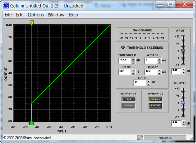
Figure 14-12    User interface for a gate, which mutes the level of signals below an adjustable threshold

When setting a gate, try the following settings. As with other DSP settings, you may need to make adjustments based on need.

•  Attack    Start with a relatively fast setting, such as 1 ms.

•  Release    Start at 50 ms.

•  Threshold    Your threshold setting depends on the gate’s position in the audio signal chain and the number of mics used. If it’s after the input gain and there is one mic, less than 0 dB is a good starting place. You may need to go lower than this if you are not getting a reliable start.

Expanders

An expander is an audio processor that comes in two forms: a downward expander or as part of what’s known as a compander.

Downward expanders increase the dynamic range by reducing—or attenuating—the level below the adjustable threshold setting. They increase gain if the signal is low, such as a presenter with a weak voice. This reduces unwanted background noise and is especially useful in a system using multiple open microphones.

Keep in mind that expanders are primarily intended for recording and transmission. When used in an amplified environment, expanders can push a system into painfully loud feedback.

Introduction to Equalization

Equalization is one of the most commonly used functions of a DSP. Equalizers, or EQs, are frequency controls that allow the user to boost (add gain) or cut (attenuate) a specific range of frequencies. The simplest equalizer comes in the form of the bass and treble tone controls found normally on your home stereo or surround receiver. The equalizer found on the input channel of a basic audio mixer may provide simple high-, mid-, and low-frequency controls.

Both the input and output signals of an audio system may be equalized. Input equalization is generally for tonality control—adjusting the tonal content so each input sounds similar. Output equalization is generally used for loudspeaker compensation—adjusting for “quirks” or characteristics of a loudspeaker’s response.

A parametric equalizer allows for the selection of a center frequency and the adjustment of the width—or Q—of the frequency range that will be affected. (The Q factor is the ratio of the height of the peak of the filter against the width of the filter at the 3 dB point; see the related Note.) This enables precise manipulation with minimal impact to the adjacent frequencies. In short, a parametric equalizer allows users to make many, large-scale adjustments to a signal with fewer filters. It offers greater flexibility than a graphic equalizer, which we will discuss later in this chapter.

Filters are classified by their rate of attenuation on the signal. This is described in terms of decibels per octave, where an octave represents a doubling of frequency. A first-order filter attenuates at a rate of 6 dB per octave.

A second-order filter attenuates at a rate of 12 dB per octave. A third-order filter attenuates at 18 dB per octave, a fourth-order filter attenuates at 24 dB per octave, and so on. Each order has 6 dB more roll-off than the one before it.

Pass Filters

A band-pass filter is a low Q filter that allows the user to eliminate the highs and lows of a frequency response. While rarely seen in professional audio gear, this type of filter is useful for tone control. Many car stereos use filters like these for bass, midrange, and treble control. Telephone lines also use band-pass filters because most telephone calls do not need to pick up a lot of bass or treble signals.

A low-pass filter is a circuit that allows signals below a specified frequency to pass unaltered while simultaneously attenuating frequencies above the specified limit. Low-pass filters are useful for eliminating hiss in a system. If you have a source with a lot of hiss, such as a low-cost consumer-level tape deck or cheap MP3 player, you can apply a low-pass filter to eliminate the high-frequency hiss.

A high-pass filter is a circuit that allows signals above a specified frequency to pass unaltered while simultaneously attenuating frequencies below the specified limit. High-pass filters are useful for removing low-frequency noise from a system, such as rumble from a heating, ventilation, and air conditioning (HVAC) system or the proximity effect on a microphone.

A shelving filter is similar to a low- or high-pass filter, except instead of removing frequency bands, it simply tapers off and flattens out the sound again. Such filters are useful when the user may want to boost or cut certain frequency bands without eliminating any sound. A boost shelf, for example, will let the user boost treble or bass in a car stereo.

Crossover Filters

Crossover filters are used for bi-amplified and tri-amplified systems. By using these filters, you can send low-, mid-, and high-range frequency bands to the appropriate, separate amplifiers. Such filters are extremely useful in large-scale concert systems for reproducing live music.

A crossover separates the audio signal into different frequency groupings and routes the appropriate material to the correct loudspeaker or amplifier to ensure that the individual loudspeaker components receive program signals that are within their optimal frequency range. Crossovers are either passive or active.

Crossover filters often use high-order, roll-off filters, often in the fourth- to eighth-order range. Bass amplifiers will often take the 250 Hz or lower range, while the high-pass filter will start at 4 KHz.

The crossover point between filters is often 3 dB. (In Figure 14-13, the crossover points are represented by the large dots between the filters.) In these areas, two different loudspeakers will reproduce that particular frequency band. Because each loudspeaker has a −3 dB cut, when they each play that sound, the sound pressure in that area will be doubled, and the audience will perceive that frequency as 0 dB.

Figure 14-13    Three crossover filters

Feedback-Suppression Filters

Feedback-suppression filters are a useful option for speech-only audio systems. They are tight-notch filters that can be used to eliminate specific bands of frequencies. (A notch filter “notches out,” or eliminates, a specific band of frequencies.) If you’ve identified a specific frequency band as a source of feedback, you can use a feedback-suppression filter to eliminate the problem.

If you have a fixed microphone in a room, such as a microphone bolted to a witness stand in a courthouse, you may find that the way the microphone interacts with reflections in the room causes feedback along specific frequencies. You can eliminate such problem areas with a feedback-suppression filter. To do so, follow these steps:

  1. Turn off all microphones except for the one you’re testing.

  2. Before you attempt the final system equalization, turn up the gain on the microphone and note the first three frequencies that cause consistent feedback.

  3. Construct three tight-notch filters at the input on those frequencies.

  4. Once you’ve created the filters, reset them and equalize the system.

Once the system has been equalized, you are ready to set your feedback-suppression filters. Simply reengage the feedback filters you identified and see whether they improve your operational-level system. Do this for every fixed microphone in your system.

Noise-Reduction Filters

A noise-reduction filter is a popular new algorithm that samples the noise floor and removes specific spectral content. It listens for noise from things such as HVAC systems, fans, other gear near microphones (such as laptops), and electronic noise. It then reduces that particular noise from the system.

The canceller depth will depend on the amount of noise present in the room. Quiet conference rooms with little or no noise may not need a noise-reduction filter, while rooms with heavy noise, such as a training room with a large audience and loud air conditioning, may need a severe noise-reduction filter. Try these settings as a starting point:

•  For eliminating computer and projector fan noise, start at 9 dB.

•  For eliminating heavy room noise, start at 12 dB.

Remember that the purpose of these filters is to remove spectral content. They are not perfect, and they will affect your room response.

Delays

A delay is the retardation of a signal. In the context of audio processing, it is an adjustment of the time in which a signal is sent to a destination, often to compensate for the distance between loudspeakers or for the differential in processing required between multiple signals. If a delay is an unintended byproduct of signal processing, it is usually referred to as latency.

Delays are used in sound systems for loudspeaker alignment—either to align components within a loudspeaker enclosure or array or to align supplemental loudspeakers with the main speakers.

Within a given loudspeaker enclosure, the individual components may be physically offset, causing differences in the arrival time from those components. This issue can be corrected either physically or by using delays to provide proper alignment.

Electronic delay is often used in sound reinforcement applications. For example, consider an auditorium with an under-balcony area. The audience seated underneath the balcony may not be covered well by the main loudspeakers. In this case, supplemental loudspeakers are installed to cover the portion of the audience seated underneath the balcony.

Although the electronic audio signal arrives at both the main and under-balcony loudspeakers simultaneously, the sound coming from these two separate locations would arrive at the audience underneath the balcony at different times and sound like an echo. This is because sound travels at about 1,130 feet per second (344 meters per second) under fairly normal temperature conditions (about 71 degrees Fahrenheit), much slower than the speed of the electronic audio signal.

In this example, an electronic delay would be used on the audio signal going to the under-balcony loudspeakers. The amount of delay would be set so that the sound both from the main loudspeakers and from the under-balcony loudspeakers arrive at the audience at the same time.

Delay can also be introduced to combat the Haas effect. The human ear has the ability to locate the origin of a sound with fairly high accuracy, based on where you hear the sound from first. Through the Haas effect—or sound precedence—you can distinguish the original source location even if there are strong echoes or reflections that may otherwise mislead you. A reflection could be 10 dB louder and you’d still correctly identify the direction of the original source.

When setting up a delay, designers can use this effect to their advantage. Rather than timing the delay of the loudspeakers to come out at the same time as the original source, add 15 ms to the delay setting (or 15 ft or 5 m). This will make the speaker generate the reinforced signal 15 ms later, which allows the listener to locate correctly the origin of the sound (the lecturer, band, and so on). Without the additional delay, the listener would perceive the source of the sound as the location of the loudspeaker, rather than the location of the original source. Just don’t exceed 25 ms. Longer might be perceived as echo and compromise intelligibility.

Graphic Equalizers

Instead of using parametric equalizers, some audio professionals prefer to use graphic equalizers. A graphic equalizer is an equalizer with an interface that resembles a graph comparing amplitude along the vertical axis and frequency along the horizontal axis. Graphic equalizers normally come in 2/3-octave or, more often, 1/3-octave filters sets. Filters are usually set on center frequencies defined by the International Organization for Standardization (ISO). Center frequencies and bandwidth are fixed for these filters, so named because the adjustments to the sliders offer a “graphic” representation of the frequency response. Active graphic equalizers can provide boost and cut capability.

The graphic equalizer in Figure 14-14 has 31 controllable filters. This type of display gives you fine control of dozens of specific frequencies, where you can grab any control and add precise amounts of boost or cut to that particular frequency.

Figure 14-14    A graphic equalizer

In Figure 14-14, the line that runs near each filter control represents the combined interaction between the filters. Do you see the bumpy, rippled area around 315 Hz? That is an area with phase interference because of the way the filters around that frequency are arranged. This represents a downside of using a graphic equalizer. Parametric equalizers will avoid these phase ripples because they use fewer, smoother filters. In addition, because they use fewer filters, parametric equalizers in DSPs tend to use less processing power than a graphic equalizer.

Chapter Review

Audio processing is a complex art, and doing it right takes practice. This chapter covered audio sources and destinations, analog versus digital audio, transport methods, DSP architecture types, signal monitoring, DSP functions, equalization, and filters. They’re all critical to an audio design that delivers what the client wants from a sound system.

Review Questions

The following questions are based on the content covered in this chapter and are intended to help reinforce the knowledge you have assimilated. These questions are not extracted from the CTS-D exam nor are they necessarily CTS-D practice exam questions. For an official CTS-D practice exam, download the Total Tester as described in Appendix D.

  1. Stereo loudspeaker systems typically use what type of signal?

A. Analog

B. RGBH

C. High gain

D. Low gain

  2. What is the advantage of converting an analog signal to digital?

A. Digital signals have more signal headroom.

B. Digital signals can address signal degradation, storage, and recording issues.

C. Digital signals carry audio and video feeds that analog will not.

D. Digital signals are more energy efficient to broadcast.

  3. When creating a schematic diagram of audio signal flow for a project, what must you include in the diagram?

A. Microphones, mixers, switchers, routers, and processors

B. Inputs, outputs, equipment rack locations, ceiling venting

C. Conduit runs, pull boxes, bends

D. Construction materials, wall panels, acoustic tiles

  4. Two types of meters typically used for signal monitoring are __________ and __________.

A. VU, PPM

B. VU, AES

C. dBU, PPM

D. EBU, SMPTE

  5. For a handheld vocal microphone, you might want set the input gain for at least __________.

A. 10 dB

B. 20 dB

C. 35 dB

D. 60 dB

  6. Which of the following is not a recommended compressor setting for speech applications?

A. Ratio: 3:1

B. Attack: 10 to 20 ms

C. Release: 20 to 50 ms

D. Threshold: 0

  7. Eighth-order filters are useful as __________.

A. Notch filters

B. Crossover filters

C. Low-pass filters

D. Shelving filters

  8. When setting a delay filter, it’s useful to know that sound travels at how many feet (meters) per second at about 70 degrees Fahrenheit?

A. 950 (390)

B. 1,001 (305)

C. 1,025 (312)

D. 1,130 (344)

Answers

  1. A. Stereo loudspeaker systems typically use analog signals.

  2. B. An advantage of converting an analog signal to digital is that digital signals can address signal degradation, storage, and recording issues.

  3. A. When creating a schematic diagram of audio signal flow, you should include microphones, mixers, switchers, routers, and processors.

  4. A. Two types of meters typically used for signal monitoring are VU (volume unit) and PPM (peak program meter).

  5. C. For a handheld vocal microphone, you might want set the input gain for at least 35 dB.

  6. C. The recommended release setting for speech applications is actually 200 to 500 ms.

  7. B. Eighth-order filters are useful as crossover filters.

  8. D. Sound travels at 1,130 feet (344 meters) per second at about 70 degrees Fahrenheit.