Protocol Processing
Our mental image of a musician is often associated with giving a recital, and our image of a researcher may involve his mulling over a problem. However, musicians spend more time in less glamorous tasks, such as practicing scales, and researchers spend more time than they wish on mundane chores, such as writing grants. Mastery of a vocation requires paying attention to many small tasks and not just to a few big jobs.
Similarly, tutorials on efficient protocol implementation often emphasize methods of avoiding data-touching overhead and structuring techniques to reduce control overhead. These, of course, were the topics covered in Chapters 5 and 6. This is entirely appropriate because the biggest improvements in endnode implementations often come from attention to such overhead.
However, having created a zero-copy implementation with minimal context switching — and there is strong evidence that modern implementations of network appliances have learned these lessons well – new bottlenecks invite scrutiny. In fact, a measurement study by Kay and Pasquale [KP93] shows that these other bottlenecks can be significant.
There are a host of other protocol implementation tasks that can become new bottlenecks. Chapters 7 and 8 have already dealt with efficient timer and demultiplexing implementations. This chapter deals briefly with some of the common remaining tasks: buffer management, checksums, sequence number bookkeeping, reassembly, and generic protocol processing.
The importance of these protocol-processing “chores” may be increasing, for the following reasons. First, link speeds in the local network are already at gigabit levels and are going higher. Second, market pressures are mounting to implement TCP, and even higher-level application tasks, such as Web services and XML, in hardware. Third, there is a large number of small packets in the Internet for which data manipulation overhead may not be the dominant factor.
This chapter is organized as follows. Section 9.1 delves into techniques for managing buffer, that is, techniques for fast buffer allocation and buffer sharing. Section 9.2 presents techniques for implementing CRCs (mostly at the link level) and checksums (mostly at the transport level). Section 9.3 deals with the efficient implementation of generic protocol processing, as exemplified by TCP and UDP. Finally, Section 9.4 covers the efficient implementation of packet reassembly.
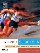
The techniques presented in this chapter (and the corresponding principles) are summarized in Figure 9.1.
9.1 BUFFER MANAGEMENT
All protocols have to manage buffers. In particular, packets travel up and down the protocol stack in buffers. The operating system must provide services to allocate and deallocate buffers. This requires managing free memory; finding memory of the appropriate size can be challenging, especially because buffer allocation must be done in real time. Section 9.1.1 describes a simple systems solution for doing buffer allocation at high speeds, even for requests of variable sizes.
If the free space must be shared between a number of connections or users, it may also be important to provide some form of fairness so that one user cannot hog all the resources. While static limits work, in some cases it may be preferable to allow dynamic buffer limits, where a process in isolation can get as many buffers as it needs but relinquishes extra buffers when other processes arrive. Section 9.1.2 describes two dynamic buffer-limiting schemes that can be implemented at high speeds.
9.1.1 Buffer Allocation
The classical BSD UNIX implementation, called mbufs, allowed a single packet to be stored as a linear list of smaller buffers, where a buffer is a contiguous area of memory.1 The motivation for this technique is to allow the space allocated to the packet to grow and shrink (for example, as it passes up and down the stack). For instance, it is easy to grow a packet by prepending a new mbuf to the current chain of mbufs. For even more flexibility, BSD mbufs come in three flavors: two small sizes (100 and 108 bytes) and one large size (2048 bytes, called a cluster).
Besides allowing dynamic expansion of a packet’s allocated memory, mbufs make efficient use of memory, something that was important around 1981, when mbufs were invented. For example, a packet of 190 bytes would be allocated two mbufs (wasting around 20 bytes), while a packet of 450 bytes would be allocated five mbufs (wasting around 50 bytes).
However, dynamic expansion of a packet’s size may be less important than it sounds because the header sizes for important packet paths (e.g., Ethernet, IP, TCP) are well known and can be preallocated. Similarly, saving memory may be less important in workstations today than increasing the speed of packet processing. On the other hand, the mbuf implementation makes accessing and copying data much harder because it may require traversing the list.
Thus very early on, Van Jacobson designed a prototype kernel that used what we called pbufs. As Jacobson put it in an email note [Jac93]: “There is exactly one, contiguous, packet per pbuf (none of that mbuf chain stupidity).”
While pbufs have sunk into oblivion, the Linux operating system currently uses a very similar idea [Cox96] for network buffers called sk_buf. These buffers, like pbufs, are linear buffers with space saved in advance for any packet headers that need to be added later. At times, this will incur wasted space to handle the worst-case headers, but the simpler implementation makes this worthwhile. Both sk_bufs and pbufs relax the specification of a buffer to avoid unnecessary generality (P7) and trade memory for time (P4b).
Given that the use of linear buffer sizes, as in Linux, is a good idea, how do we allocate memory for packets of various sizes? Dynamic memory allocation is a hard problem in general because users (e.g., TCP connections) deallocate at different times, and these deallocations can fragment memory into a patchwork of holes of different sizes.
The standard textbook algorithms, such as First-Fit and Best-Fit [WJea95], effectively stroll through memory looking for a hole of the appropriate size. Any implementor of a highspeed networking implementation, say, TCP, should be filled with horror at the thought of using such allocators. Instead, the following three allocators should be considered.
SEGREGATED POOL ALLOCATOR
One of the fastest allocators, due to Chris Kingsley, was distributed along with BSD 4.2 UNIX. Kingsley’s malloc() implementation splits all of memory into a set of segregated pools of memory in powers of 2. Any request is rounded up to its closest power of 2, a table lookup is done to find the corresponding pool list, and a buffer is allocated from the head of that list if available. The pools are said to be segregated because when a request of a certain size fails there is no attempt made to carve up available larger buffers or to coalesce contiguous smaller buffers.
Such carving up and coalescing is actually done by a more classical scheme called the buddy system (see Wilson et al. [WJea95] for a thorough review of memory allocators). Refraining from doing so clearly wastes memory (P4b, trading memory for speed). If all the requests are for exactly one pool size, then the other pools are wasted. However, this restraint is not as bad as it seems because allocators using the buddy system have a far more horrible worst case.
Suppose, for example, that all requests are for size 1 and that every alternate buffer is than deallocated. Then, using the buddy system, memory degenerates into a series of holes of size 1 followed by an allocation of size 1. Half of memory is unused, but no request of size greater than 2 can be satisfied. Notice that this example cannot happen with the Kingsley allocator because the size-1 requests will only deplete the size-1 pool and will not affect the other pools. Thus trafficking between pools may help improve the expected memory utilization but not the worst-case utilization.
LINUX ALLOCATOR
The Linux allocator [Che01], originally written by Doug Lea, is sometimes referred to as dlmalloc(). Like the Kingsley allocator, the memory is broken into pools of 128 sizes. The first 64 pools contain memory buffers of exactly one size each, from 16 through 512 bytes in steps of 8. Unlike the case of power-of-2 allocation, this prevents more than 8 bytes of waste for the common case of small buffers. The remaining 64 pools cover the other, higher sizes, spaced exponentially.
The Linux allocator [Che01] does merge adjacent free buffers and promotes the coalesced buffer to the appropriate pool. This is similar to the buddy system and hence is subject to the same fragmentation problem of any scheme in which the pools are not segregated. However, the resulting memory utilization is very good in practice.
A useful trick to tuck away in your bag of tricks concerns how pools are linked together. The naive way would be to create separate free lists for each pool using additional small nodes that point to the corresponding free buffer. But since the buffer is free, this is obvious waste (P1). Thus the simple trick, used in Linux and possibly in other allocators, is to store the link pointers for the pool free lists in the corresponding free buffers themselves, thereby saving storage.
The Lea allocator uses memory more efficiently than the Kingsley allocator but is more complex to implement. This may not be the best choice for a wire-speed TCP implementation that desires both speed and the efficient use of memory.
BATCH ALLOCATOR
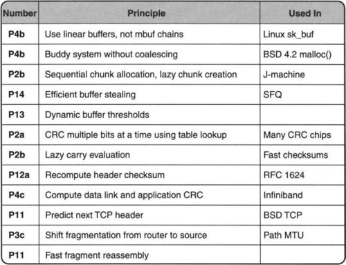
One alternative idea for memory allocation, which has an even simpler hardware implementation than Kingsley’s allocator, leverages batching (P2c). The idea, shown in Figure 9.2, is for the allocator to work in large chunks of memory. Each chunk is allocated sequentially. A pointer Curr is kept to the point where the last allocation terminated. A new request of size B is allocated after Curr, and Curr increases to Curr + B. This is extremely fast, handles variable sizes, and does not waste any memory — up to the point, that is, when the chunk is used up.
The idea is that when the chunk is used up, another chunk is immediately available. Of course, there is no free lunch — while the second chunk is being used, some spare chunk must be created in the background. The creation of this spare chunk can be done by software, while allocates can easily be done in hardware. Similar ideas were presented in the context of the MIT J-machine [DCea87], which relied on an underlying fast messaging service.
Creating a spare chunk can be done in many ways. The problem, of course, is that deallocates may not be done in the same order as allocates, thus creating a set of holes in the chunks that need somehow to be coalesced. Three alternatives for coalescing present themselves. If the application knows that eventually all allocated buffers will be freed, then using some more spare chunks may suffice to ensure that before any chunk runs out some chunk will be completely scavenged. However, this is a dangerous game.
Second, if memory is accessed through a level of indirection, as in virtual memory, and the buffers are allocated in virtual memory, it is possible to use page remapping to gather together many scattered physical memory pages to appear as one contiguous virtual memory chunk. Finally, it may be worth considering compaction. Compaction is clearly unacceptable in a general-purpose allocator like UNIX, where any number of pieces of memory may point to a memory node. However, in network applications using buffers or other treelike structures, compaction may be feasible using simple local compaction schemes [SV00].
9.1.2 Sharing Buffers
If buffer allocation was not hard enough, consider making it harder by asking also for a fairness constraint.2 Imagine that an implementation wishes to fairly share a group of buffers among a number of users, each of whom may wish to use all the buffers. The buffers should be shared roughly equally among the active users that need these buffers. This is akin to what in economics is called Pareto optimality and also to the requirements for fair queuing in routers studied in Chapter 14. Thus it is not surprising that the following buffer-stealing algorithm was invented [McK91] in the context of a stochastic fair queuing (SFQ) algorithm.
BUFFER STEALING
One way to provide roughly Pareto optimality among users is as follows. When all buffers are used up and a new user (whose allocated buffers are smaller than the highest current allocation) wishes one more buffer, steal the extra buffer from the highest buffer user. It is easy to see that even if one user initially grabs all the buffers when other users become active, they can get their fair share by stealing.
The problem is that a general solution to the problem of buffer stealing uses a heap. A heap has O(log n) cost, where n is the number of users with current allocations. How can this be made faster?
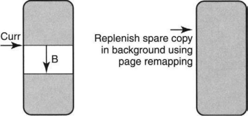
Once again, as is often the case in algorithmics versus algorithms, the problem is caused by reading too much into the specification. If allocations keep changing in arbitrary increments and the algorithm wishes always to find the highest allocation, a logarithmic heap implementation is required. However, if we can relax the specification (and this seems reasonable in practice) to assume that a user steals one buffer at a time, then the allocated amounts change not in arbitrary amounts but only by + 1 or –1. This observation results in a constant-time algorithm (the Mckenney algorithm, Figure 9.3), which also assumes that buffer allocations fall in a bounded set. For each allocation size i, the algorithm maintains a list of processes that have size exactly i. The algorithm maintains a variable called Highest that points to the highest amount allocated to any process.
When a process P wishes to steal a buffer, the algorithm finds a process Q with the highest allocation at the head of the list pointed to by Highest. While doing so, process P gains a buffer and Q loses a buffer. The books are updated as follows.
When process P gets buffer i + 1, P is removed from list i and added to list i + 1, updating Highest if necessary. When process Q loses buffer i + 1, Q is removed from list i + 1 and added to list i, updating Highest = i if the Highest list becomes empty.
Notice this could become arbitrarily inefficient if P and Q could change their allocations by sizes larger than 1. If Q could reduce its allocation by, say, 100 and there are no other users with the same original allocation, then the algorithm would require stepping through 100 lists, looking for the next possible value of highest. Because the maximum amount an allocation can change by is 1, the algorithm moves through only one list. In terms of algorithmics, this is an example of the special opportunities created by the use of finite universes (P14 suggests the use of bucket sorting and bitmaps for finite universes).
DYNAMIC THRESHOLDS
Limiting access by any one flow to a shared buffer is also important in shared memory switches (Chapter 13). In the context of shared memory switches, Choudhury and Hahne describe an algorithm similar to buffer stealing that they call Pushout. However, even using the buffer-stealing algorithm due to McKenney [McK91], Pushout may be hard to implement at high speeds.
Instead, Choudhury and Hahne [CH98] propose a useful alternative mechanism called dynamic buffer limiting. They observe that maintaining a single threshold for every flow is either overly limiting (if the threshold is too small) or unduly dangerous (if the threshold is too high). Using a static value of threshold is no different from using a fixed window size for flow control. But TCP uses a dynamic window size that adapts to congestion. Similarly, it makes sense to exploit a degree of freedom (P13) and use dynamic thresholds.
Intuitively, TCP window flow control increases a connection’s window size if there appears to be unused bandwidth, as measured by the lack of packet drops. Similarly, the simplest way to adapt to congestion in a shared buffer is to monitor the free space remaining and to increase the threshold proportional to the free space. Thus user i is limited to no more than cF bytes, where c is a constant and F is the current amount of free space. If c is chosen to be a power of 2, this scheme only requires the use of a shifter (to multiply by c) and a comparator (to compare with cF). This is far simpler than even the buffer-stealing algorithm.
Choudhury and Hahne recommend a value of c = 1. This implies that a single user is limited to taking no more than half the available bandwidth. This is because when the user takes half, the free space is equal to the user allocation and the threshold check fails. Similarly, if c = 2, any user is limited to no more than 2/3 of the available buffer space. Thus unlike buffer stealing, this scheme always holds some free space in reserve for new arrivals, trading slightly suboptimal use of memory for a simpler implementation.
Now suppose there are two users and that c = 1. One might naively think that since each user is limited to no more than half, two active users are limited to a quarter. The scheme does better, however. Each user now can take 1/3, leaving 1/3 free. Next, if two new users arrive and the old users do not free their buffers, the two new users can get up to 1/9 of the buffer space.
Thus, unlike buffer stealing, the scheme is not fair in a short-term sense. However, if the same set of users is present for sufficiently long periods, the scheme should be fair in a longterm sense. In the previous example, after the buffers allocated to the first two users are deallocated, a fairer allocation should result.
9.2 CYCLIC REDUNDANCY CHECKS AND CHECKSUMS
Once a TCP packet is buffered, typically a check is performed to see whether the packet has been corrupted in flight or in a router’s memory. Such checks are performed by either checksums or cyclic redundancy checks (CRCs). In essence, both CRCs and checksums are hash functions H on the packet contents. They are designed so that if errors convert a packet P to corrupted packet P′, then H(P) ≠ H(P′) with high probability.
In practice, every time a packet is sent along a link, the data link header carries a link level CRC. But in addition, TCP computes a checksum on the TCP data. Thus a typical TCP packet on a wire carries both a CRC and a checksum. While this may appear to be obvious waste (P1), it is a consequence of layering. The data link CRC covers the data link header, which changes from hop to hop. Since the data link header must be recomputed at each router on the path, the CRC does not catch errors caused within routers. While this may seem unlikely, routers do occasionally corrupt packets [SP00] because of implementation bugs and hardware glitches.
Given this, the CRC is often calculated in hardware by the chip (e.g., Ethernet receiver) that receives the packet, while the TCP checksum is calculated in software in BSD UNIX. This division of labor explains why CRC and checksum implementations are so different. CRCs are designed to be powerful error-detection codes, catching link errors such as burst errors. Checksums, on the other hand, are less adept at catching errors; however, they tend to catch common end-to-end errors and are much simpler to implement in software.
The rest of this section describes CRC and then checksum implementation. The section ends with a clever way, used in Infiniband implementations, to finesse the need for software checksums by using two CRCs in each packet, both of which can easily be calculated by the same piece of hardware.
9.2.1 Cyclic Redundancy Checks
The CRC “hash” function is calculated by dividing the packet data, treated as a number, with a fixed generator G. G is just a binary string of predefined length. For example, CRC-16 is the string 11000000000000101, of length 17; it is called CRC-16 because the remainder added to the packet turns out to be 16 bits long.
Generators are easier to remember when written in polynomial form. For example, the same CRC-16 in polynomial form becomes x16 + x15 + x2 + 1. Notice that whenever xi is present in the generator polynomial, position i is equal to 1 in the generator string. Whatever CRC polynomial is picked (and CRC-32 is very common), the polynomial is published in the data link implementation specification and is known in advance to both receiver and sender.
A formal description of CRC calculation is as follows. Let r be the number of bits in the generator string G. Let M be the message whose CRC is to be calculated. The CRC is simply the remainder c of 2r−1M (i.e., M left-shifted by r – 1 bits) when divided by G. The only catch is the division is mod-2 division, which is illustrated next.
Working out the mathematics slightly, 2r–1M = k.G + c. Thus 2r−1M + c = k.G because addition is the same as subtraction in mod-2 arithmetic, a fact strange but true. Thus, even ignoring the preceding math, the bottom line is that if we append the calculated CRC c to the end of the message, the resulting number divides the generator G.
Any bit errors that cause the sent packet to change to some other packet will be caught as long as the resulting packet is not divisible by G. CRCs, like good hash functions, are effective because common errors based on flipping a few bits (random errors) or changing any bit in a group of contiguous bits (burst errors) are likely to create a packet that does not divide G. Simple analytical properties of CRCs are derived in Tanenbaum [Tan81].
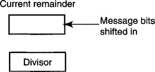
For the implementor, however, what matters is not why CRC works but how to implement it. The main thing to learn is how to compute remainders using mod-2 division. The algorithm uses a simple iteration in which the generator G is progressively “subtracted” from the message M until the remainder is “smaller” than the generator G. This is exactly like ordinary division except that “subtraction” is now exclusive-OR, and the definition of whether a number is “smaller” depends on whether its most significant bit (MSB) is 0.
More precisely, a register R is loaded with the first r bits of the message. At each stage of the iteration, the MSB of R is checked. If it is 1, R is “too large” and the CRC string G is “subtracted” from R. Subtraction is done by exclusive-OR (EX-OR) in mod-2 arithmetic. Assuming that the MSB of the generator is always 1, this zeroes out the MSB of R. Finally, if the MSB of R is already 0, R is “small enough” and there is no need to EX-OR.
A single iteration completes by left-shifting R so that the MSB of R is lost, and the next message bit gets shifted in. The iterations continue until all messages are shifted in and the MSB of register R is 0. At this point register R contains the required checksum.
For example, let M = 110 and G = 111. Then 2r–1M = 11000. Then the checksum c is calculated as shown in Figure 9.4. In the first step of Figure 9.4, the algorithm places the first 3 bits (110) of the shifted message in R. Since the MSB of 110 is 1, the algorithm hammers away at R by EX-ORing R with the generator G = 111 to get 001. The first iteration completes by shifting out the MSB and (Figure 9.4, topmost vertical arrow) shifting in the fourth message bit, to get R = 010.
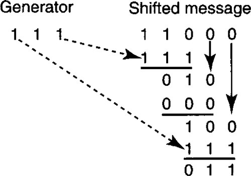
In the second iteration, the MSB of R is 0 and so the algorithm desists. This is represented in Figure 9.4 by computing the EX-OR of R with 000 instead of the generator. As usual, the MSB of the result is shifted in, and the last message bit, also a zero, is shifted in to get R = 100. Finally, in the third iteration, because the MSB of R is 1, the algorithm once again EX-ORs R with the generator. The algorithm terminates at this point because the MSB of R is 0. The resulting checksum is R without the MSB, or 11.
NAIVE IMPLEMENTATION
Cyclic redundancy checks have to be implemented at a range of speeds from 1 Gbit/sec to slower rates. Higher-speed implementations are typically done in hardware. The simplest hardware implementation would mimic the foregoing description and use a shift register that shifts in bits one at time. Each iteration requires three basic steps: checking the MSB, computing the EX-OR, and then shifting.
The naive hardware implementation shown in Figure 9.5 would require three clock cycles to shift in a bit; doing a comparison for the MSB in one cycle and the actual EX-OR in another cycle and the shift in the third cycle. However, a cleverer implementation can be used to shift in one bit every clock cycle by combining the test for MSB, the EX-OR, and the shift into a single operation.
IMPLEMENTATION USING LINEAR FEEDBACK SHIFT REGISTERS
In Figure 9.6 the remainder R is stored as five separate 1-bit registers, R4 through R0, instead of a single 5-bit register, assuming a 6-bit generator string. The idea makes use of the observation that the EX-OR needs to be done only if the MSB is 1; thus in the process of shifting left the MSB, we can feed back the MSB to the appropriate bits of the remainder register. The remaining bits are EX-ORed during their shift to the left.
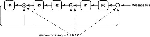
Notice that in Figure 9.6, an EX-OR gate is placed to the right of register i if bit i in the generator string (see dashed lines) is set. The reason for this rule is as follows. Compared to the simple iterative algorithm, the hardware of Figure 9.6 effectively combines the left shift of iteration J together with the MSB check and EX-OR of iteration J + 1. Thus the bit that will be in position i in iteration J + 1 is in position i – 1 in iteration J.
If this is grasped (and this requires shifting one’s mental pictures of iterations), the test for the MSB (i.e., bit 5) in iteration J + 1 amounts to checking MSB – 1 (i.e., bit 4 in R4) in iteration J. If bit 4 is 1, then an EX-OR must be performed with the generator. For example, the generator string has a 1 in bit 2, so R2 must be EX-ORed with a 1 in iteration J + 1. But bit 2 in iteration J + 1 corresponds to bit 1 in iteration J. Thus the EX-OR corresponding to R2 in iteration J + 1 can be achieved by placing an EX-OR gate to the right of R2: The bit that will be placed in R2 is EX-ORed during its transit from R1.
Notice that the check for MSB has been finessed in Figure 9.6 by using the output of R4 as an input to all the EX-OR gates. The effect of this is that if the MSB of iteration J + 1 is 1 (recall that this is in R4 during iteration J), then all the EX-ORs are performed. If not, and if the MSB is 0, no EX-ORs are done, as desired; this is the same as EX-ORing with zero in Figure 9.4.
The implementation of Figure 9.6 is called a linear feedback shift register (LFSR), for obvious reasons. This is a classical hardware building block, which is also useful for the generation of random numbers for, say, QoS (Chapter 14). For example, random numbers using, say, the Tausworth implementation can be generated using three LFSRs and an EX-OR.
FASTER IMPLEMENTATIONS
The bottleneck in the implementation of Figure 9.6 is the shifting, which is done one bit at a time. Even at one bit every clock cycle, this is very slow for fast links. Most logic on packets occurs after the bit stream arriving from the link has been deserialized3 into wider words of, say, size W. Thus the packet-processing logic is able to operate on W bits in a single clock cycle, which allows the hardware clock to run W times slower than the interarrival time between bits.
Thus to gain speed, CRC implementations have to shift W bits at a time, for W > 1. Suppose the current remainder is r and we shift in W more message bits whose value as a number is, say, n. Then in essence the implementation needs to find the remainder of (2W ·r + n) in one clock cycle.
If the number of bits in the current remainder register is small, the remainder of 2w ·r can be precomputed (P2a) for all r by table lookup. This is the basis of a number of software CRC implementations that shift in, say, 8 bits at a time. In hardware, it is faster and more space efficient to use a matrix of XOR gates to do the same computation. The details of the parallel implementation can be found in Albertengo and Riccardo [AR90], based on the original idea described by Sarwate [Sar88].
9.2.2 Internet Checksums
Since CRC computation is done on every link in the Internet, it is done in hardware by link chips. However, the software algorithm, even shifting 8 bits at a time, is slow. Thus TCP chose to use a more efficient error-detection hash function based on summing the message bits. Just as accountants calculate sums of large sets of numbers by column and by row to check for errors, a checksum can catch errors that change the resulting sum.
It is natural to calculate the sum in units of the checksum size (16 bits in TCP), and some reasonable strategy must be followed when the sum of the 16-bit units in the message overflows the checksum size. Simply losing the MSB will, intuitively, lose information about 16-bit chunks computed early in the summing process. Thus TCP follows the strategy of an end-around carry. When the MSB overflows, the carry is added to the least significant bit (LSB). This is called one’s complement addition.
The computation is straightforward. The specified portion of each TCP packet is summed in 16-bit chunks. Each time the sum overflows, the carry is added to the LSB. Thus the main loop will naively consist of three steps: Add the next chunk; test for carry; if carry, add to LSB. However, there are three problems with the naive implementation.
• Byte Swapping: First, in some machines, the 16-bit chunks in the TCP message may be stored byte-swapped. Thus it may appear that the implementation has to reverse each pair of bytes before addition.
• Masking: Second, many machines use word sizes of 32 bits or larger. Thus the naive computation may require masking out 16-bit portions.
• Check for Carry: Third, the check for carry after every 16-bit word is added can potentially slow down the loop as compared to ordinary summation.
All three problems can be solved by not being tied to the reference implementation (P8) and, instead, by fitting the computation to the underlying hardware (P4c). The following ideas and Figure 9.7 are taken from Partridge [Par93].
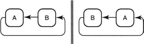
• Ignore byte order: Figure 9.7 shows that swapping every word before addition on a byte-reversed machine is obvious waste (P1). The figure shows that whether or not AB is stored byte reversed as BA, any carry from the MSB of byte B still flows to the LSB of byte A. Similarly, in both cases, any carry from the MSB of byte A flows to the LSB of byte B. Thus any 1’s-complement addition done on the byte-reversed representation will have the same answer as in the original, except byte reversed. This in turn implies that it suffices to add in byte-reversed form and to do a final byte reversal only at the end.
• Use natural word length: If a machine has a 32 -or 64-bit word, the most natural thing to do is to maintain the running sum in the natural machine word size. All that happens is that carries accumulate in the higher-order 16 bits of the machine word, which need to be added back to the lower 16 bits in a final operation.
• Lazy carry evaluation: Using a larger word size has the nice side effect of allowing lazy evaluation (P2b) of carry checking. For example, using a 32-bit word allows an unrolled loop that checks for carries only after every 16 additions [Ste94], because it takes 16 additions in the worst case to have the carry overflow from bit 32.
In addition, as noted in Chapter 5, the overhead of reading in the checksum data into machine registers can be avoided by piggybacking on the same requirement for copying data from the network device into user buffers, and vice versa.
HEADER CHECKSUM
Finally, besides the TCP and UDP checksums on the data, IP computes an additional 1’s complement checksum on just the IP header. This is crucial for network routers and other hardware devices that need to recompute Internet checksums.
Hardware implementations of header checksum can benefit from parallel and incremental computation. One strategy for parallelism is to break up the data being checksummed into W 16-bit words and to compute W different 1 ’s-complement sums in parallel, with a final operation to fold these W sums into one 16-bit checksum. A complete hardware implementation of this idea with W = 2 is described in Touch and Parham [TP96].
The strategy for incremental computation is defined precisely in RFC 1624 [Rij94]. In essence, if a 16-bit field m in the header changes to m′, the header checksum can be recalculated by subtracting m and adding in m′ to the older checksum value. There is one subtlety, having to do with the two representations of zero in 1’s-complement arithmetic [Rij94], that is considered further in the exercises.
9.2.3 Finessing Checksums
The humble checksum’s reason for existence, compared to the more powerful CRC, is the relative ease of checksum implementation in software. However, if there is hardware that already computes a data link CRC on every data link frame, an obvious question is: Why not use the underlying hardware to compute another checksum on the data? Doing otherwise results in extra computation by the receiving processor and appears to be obvious waste (P1). Once again, it is only obvious waste when looking across layers; at each individual layer (data link, transport) there is no waste.
Clearly, the CRC changes from hop to hop, while the TCP checksum should remain unchanged to check for end-to-end integrity. Thus if a CRC is to be used for both purposes, two CRCs have to be computed. The first is the usual CRC, and the second should be on some invariant portion of the packet that includes all the data and does not change from hop to hop.
One of the problems with exploiting the hardware (P4c) to compute the equivalent of the TCP checksum is knowing which portion of the packet must be checksummed. For example, TCP and UDP include some fields of the IP header4 in order to compute the end-to-end checksum. The TCP header fields may also not be at a fixed offset because of potential TCP and IP options. Having a data link hardware device understand details of higher-layer headers seems to violate layering.
On the other hand, all the optimizations that avoid data copying and described in Chapter 5 also violate layering in a similar sense. Arguably, it does not matter what a single endnode does internally as long as the protocol behavior, as viewed externally by a black-box tester, meets conformance tests. Further, there are creative structuring techniques (P8, not being tied to reference implementations) of the endnode software that can allow lower layers access to this form of information.
The Infiniband architecture [AS00] does specify that end system hardware compute two CRCs. The usual CRC is called the variant CRC; the CRC on the data, together with some of the header, is called the invariant CRC. Infiniband transport and network layer headers are simpler than those of TCP, and thus computing the invariant portion is fairly simple.
However, the same idea could be used even for a more complex protocol, such as TCP or IP, while preserving endnode software structure. This can be achieved by having the upper layers pass information about offsets and fields (P9) to the lower layers through layer interfaces. A second option to avoid passing too many field descriptions is to precompute the pseudoheader checksum/CRC as part of the connection state [Jac93] and instead to pass the precomputed value to the hardware.
9.3 GENERIC PROTOCOL PROCESSING
Section 9.1 described techniques for buffering a packet, and Section 9.2 described techniques to efficiently compute packet checksums. The stage is now set to actually process such a packet. The reader unfamiliar with TCP may wish first to consult the models in Chapter 2.
Since TCP accounts for 90% of traffic [Bra98] in most sites, it is crucial to efficiently process TCP packets at close to wire speeds. Unfortunately, a first glance at TCP code is daunting. While the TCP sender code is relatively simple, Stevens [Ste94] says:
TCP input processing is the largest piece of code that we examine in this text. The function tcp_input is about 1100 lines of code. The processing of incoming segments is not complicated, just long and detailed.
Since TCP appears to be complex, Greg Chesson and Larry Green formed Protocol Engines, Inc., in 1987, which proposed an alternative protocol called XTP [Che89]. XTP was carefully designed with packet headers that were easy to parse and streamlined processing paths. With XTP threatening to replace TCP, Van Jacobson riposted with a carefully tuned implementation of TCP in BSD UNIX that is well described in Stevens [Ste94]. This implementation was able to keep up with even 100-Mbps links. As a result, while XTP is still used [Che89], TCP proved to be a runaway success.
Central to Jacobson’s optimized implementation is a mechanism called header prediction [Jac93]. Much of the complexity of the 1100 lines of TCP receive processing comes when handling rare cases. Header prediction provides a fast path through the thicket of exceptions by optimizing the expected case (P11).
TCP HEADER PREDICTION
The first operation on receiving a TCP packet is to find the protocol control block (PCB) that contains the state (e.g., receive and sent sequence numbers) for the connection of which the packet is a part. Assuming the connection is set up and that most workstations have only a few concurrent connections, the few active connection blocks can be cached. The BSD UNIX code [Ste94] maintains a one-behind cache containing the PCB of the last segment received; this works well in practice for workstation implementations.
After locating the PCB, the TCP header must be processed. A good way to motivate header prediction, found in Partridge [Par93], comes from looking at the fields in the TCP header, as shown in Figure 9.8.
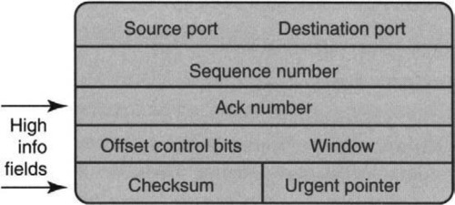
After a connection is set up, the destination and source ports are fixed. Since IP networks work hard to send packets in order, the sequence number is likely to be the next in sequence after the last packet received. The control bits, often called flag bits, are typically off, with the exception of the ack bit, which is always set after the initial packet is sent. Finally, most of the time the receiver does not change its window size, and the urgent pointer is irrelevant. Thus the only two fields whose information content is high are the ack number and checksum fields.
Motivated by this observation, header prediction identifies the expected case as one of two possibilities: receiving a pure acknowledgment (i.e., the received segment contains no data) or receiving a pure data packet (i.e., the received segment contains an ack field that conveys no new information). In addition, the packet should also reflect business as usual in the following precise sense: No unexpected TCP flags should be set, and the flow control window advertised in the packet should be no different from what the receiver had previously advertised. In pseudocode (simplified from Ref. Jac93):
IF (No unexpected flags) AND (Window in packet is as before)
AND (Packet sequence number is the next expected) THEN
IF (Packet contains only headers and no data)
Do Ack Processing
/* Release acked bytes, stop timers, awaken process */
ELSE IF (Packet does not ack anything new) /* pure data */
Copy data to user buffer while checksumming;
Update next sequence number expected;
Send Acks if needed and release buffer;
ENDIF
ELSE /* header prediction failed -- take long path */
...
Clearly, this code is considerably shorter than the complete TCP receive processing code. However, some of the checks can be made more efficient by leveraging off the fact that most machines can do efficient comparisons in units of a machine word size (P4a, exploit locality).
For example, consider the TCP flags contained in the control bits of Figure 9.8. There are six flags, each encoded as a bit: SYN, FIN, RESET, PUSH, URG, ACK. If it is business as usual, all the flags must be clear, with the exception of ACK, which must be set, and PUSH, which is irrelevant. Checking for each of these conditions individually would require several instructions to extract and compare each bit.
Instead, observe that the flags field is the fourth word of the TCP header and that the window size is contained in the last 16 bits. In the header prediction code, the sender precomputes (P2a) the expected value of this word by filling in all the expected values of the flag and using the last advertised value of the window size.
The expected value of the fourth TCP header word is stored in the PCB entry for the connection. Given this setup, the first two checks in the pseudocode shown earlier can be accomplished in one stroke by comparing the fourth word of the TCP header in the incoming packet with the expected value stored in the PCB. If all goes well, and tests indicate they often do, the expected value of the fourth field is computed only at the start of the connection. It is this test that explains the origin of the name header prediction: A portion of the header is being predicted and checked against an incoming segment.
The pseudocode described earlier is abstracted from the implementation by Jacobson in a research kernel [Jac93] that claims to do TCP receiving processing in 30 Sun SPARC instructions! The BSD UNIX code given in Stevens [Ste94] is slightly more complicated, having to deal with mbufs and with the need to eliminate other possibilities, such as the PAWS test [Ste94].
The discussion so far has been limited to TCP receive processing because it is more complex than sending a TCP segment. However, a dual of header prediction exists for the sender side. If only a few fields change between segments, the sender may benefit from keeping a template TCP (and IP) header in the connection block. When sending a segment, the sender need only fill in the few fields that change into the template. This is more efficient if copying the TCP header is more efficient than filling in each field. Caching of sending packet headers is implemented in the Linux kernel.
Before finishing this topic, it is worth recalling Caveat Q8 and examining how sensitive this optimization is to the system environment. Originally, header prediction was targeted at workstations. The underlying assumption (that the next segment is for the same connection and is one higher in sequence number than the last received segment) works well in this case.
Clearly, the assumption that the next segment is for the same connection works poorly in a server environment. This was noted as early as Jacobson [Jac93], who suggested using a hash of the port numbers to quickly locate the protocol control block. McKenney and Dove confirmed this by showing that using hashing to locate the PCB can speed up receive processing by an order of magnitude in an OLTP (online transaction processing) environment
The FIFO assumption is much harder to work around. While some clever schemes can be used to do sequence number processing for out-of-order packets, there are some more fundamental protocol mechanisms in TCP that build on the FIFO assumption. For example, if packets can be routinely misordered, TCP receivers will send duplicate acknowledgments. In TCP’s fast retransmit algorithm [Ste94], TCP senders use three duplicate acknowledgments to infer a loss (see Chapter 14).
Thus lack of FIFO behavior can cause spurious retransmissions, which will lower performance more drastically as compared to the failure of header prediction. However, as TCP receivers evolve to do selective acknowledgment [FMM+99], this could allow fast TCP processing of out-of-order segments in the future.
9.3.1 UDP Processing
Recall that UDP is TCP without error recovery, congestion control, or connection management. As with TCP, UDP allows multiplexing and demultiplexing using port numbers. Thus UDP allows applications to send IP datagrams without the complexity of TCP. Although TCP is by far the dominant protocol, many important applications, such as videoconferencing, use UDP. Thus it is also important to optimize UDP implementations.
Because UDP is stateless, header prediction is not relevant: One cannot store past headers that can be used to predict future headers. However, UDP shares with TCP two potentially time-consuming tasks: demultiplexing to the right protocol control block, and checksumming, both of which can benefit from TCP-style optimizations [PP93].
Caching of PCB entries is more subtle in UDP than in TCP. This is because PCBs may need to be looked up using wildcarded entries for, say, the remote (called foreign) IP address and port. Thus there may be PCB 1 that specifies local port L with all the other fields wildcarded, and PCB 2 that specifies local port L and remote IP address X. If PCB 1 is cached and a packet arrives destined for PCB 2, then the cache can result in demultiplexing the packet for the wrong PCB. Thus caching of wildcarded entries is not possible in general; address prefixes cannot be cached for purposes of route lookup (Chapter 11), for similar reasons.
Partridge and Pink [PP93] suggest a simple strategy to get around this issue. A PCB entry, such as PCB 1, that can “hide” or match another PCB entry is never allowed to be cached. Subject to this restriction, the UDP implementation of Partridge and Pink [PP93] caches both the PCB of the last packet received and the PCB of the last packet sent. The first cache handles the case of a train of received packets, while the second cache handles the common case of receiving a response to the last packet sent. Despite the cache restrictions, these two caches still have an 87% hit rate in the measurements of Partridge and Pink [PP93].
Finally, Partridge and Pink [PP93] also implemented a copy-and-checksum loop for UDP as in TCP. In the BSD implementation, UDP’s sosend was treated as a special case of sending over a connected socket. Instead, Partridge and Pink propose an efficient special-purpose routine that first calculates the header checksum and then copies the data bytes to the network buffer while updating the checksum. (Some of these ideas allowed Cray machines to vectorize the checksum loop in the early 1990s.) With similar optimizations used for receive processing, Partridge and Pink report that the checksum cost is essentially zero for CPUs that are limited by memory access time and not processing.
9.4 REASSEMBLY
Both header prediction for TCP and even the UDP optimizations of Partridge and Pink [PP93] assume that the received data stream has no unusual need for computation. For example, TCP segments are assumed not to contain window size changes or to have flags set that need attention. Besides these, an unstated assumption so far is that the IP packets do not need to be reassembled.
Briefly, the original IP routing protocol dealt with diverse links with different maximum packet sizes or Maximum Transmission Units (MTUs) by allowing routers to slice up IP packets into fragments. Each fragment is identified by a packet ID, a start byte offset into the original packet, and a fragment length. The last fragment has a bit set to indicate it is the last. Note that an intermediate router can cause a fragment to be itself fragmented into multiple smaller fragments. IP routing can also cause duplicates, loss, and out-of-order receipt of fragments.
At the receiver, Humpty Dumpty (i.e., the original packet) can be put together as follows. The first fragment to arrive at the receiver sets up the state that is indexed by the corresponding packet ID. Subsequent fragments are steered to the same piece of state (e.g., a linked list of fragments based on the packet ID). The receiver can tell when the packet is complete if the last fragment has been received and if the remaining fragments cover all the bytes in the original packets length, as indicated by each fragment’s offset. If the packet is not reassembled after a specified time has elapsed, the state is timed out.
While fragmentation allows IP to deal with links of different MTU sizes, it has the following disadvantages [KM87]. First, it is expensive for a router to fragment a packet because it involves adding a new IP header for fragment, which increases the processing and memory bandwidth needs. Second, reassembly at endnodes is considered expensive because determining when a complete packet has been assembled potentially requires sorting the received fragments. Third, the loss of a fragment leads to the loss of a packet; thus when a fragment is lost, transmission of the remaining fragments is a waste of resources.
The current Internet strategy [KM87] is to shift the fragmentation computation in space (P3c) from the router and the receiver to the sender. The idea behind the so-called path MTU scheme is that the onus falls on the sender to compute a packet size that is small enough to pass through all links in the path from sender to receiver. Routers can now refuse to fragment a packet, sending back a control message to the receiver. The sender uses a list of common packet sizes (P11, optimizing the expected case) and works its way down this list when it receives a refusal.
The path MTU scheme nicely illustrates algorithmics in action by removing a problem by moving to another part of the system. However, a misconception has arisen that path MTU has completely removed fragmentation in the Internet. This is not so. Almost all core routers support fragmentation in hardware, and a significant amount of fragmented traffic has been observed [SMC01] on Internet backbone links many years after the path MTU protocol was deployed.
Note that the path MTU protocol requires the sender to keep state as to the best current packet size to use. This works well if the sender uses TCP, but not if the sender uses UDP, which is stateless. In the case of UDP, path MTU can be implemented only if the application above UDP keeps the necessary state and implements path MTU. This is harder to deploy because it is harder to change many applications, unlike changing just TCP. Thus at the time of writing, shared file system protocols such as NFS, IP within IP encapsulation protocols, and many media player and game protocols run over UDP and do not support path MTU. Finally, many attackers compromise security by splitting an attack payload across multiple fragments. Thus intrusion detection devices must often reassemble IP fragments to check for suspicious strings within the reassembled data.
Thus it is worth investigating fast reassembly algorithms because common programs such as NFS do not support the path MTU protocol and because real-time intrusion detection systems must reassemble packets at line speeds to detect attacks hidden across fragments. The next section describes fast reassembly implementations at receivers.
9.4.1 Efficient Reassembly
Figure 9.9 shows a simple data structure, akin to the one used in BSD UNIX, for reassembling a data packet. Assume that three fragments for the packet with ID 1080 have arrived. The fragments are sorted in a list by their starting offset number. Notice that there are overlapping bytes because the first fragment contains bytes 1–10, while the second contains 2–21.
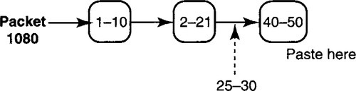
Thus if a new fragment with packet ID 1080 arrives containing offsets 25–30, the implementation will typically search through the list, starting from the head, to find the correct position. The correct position is between start offsets 2 and 40 and so is after the second list item.
Each time a fragment is placed in the list, the implementation can check during list traversal if all required bytes have been received up to this fragment. If so, it continues checking to the end of the list to see if all bytes have been received and the last fragment has the last fragment bit set. If these conditions are met, then all required fragments have arrived; the implementation then traverses the list again, copying the data of each fragment into another buffer at the specified offset, potentially avoiding copying overlapping portions.
The resulting implementation is quite complex and slow and typically requires an extra copy. Note that to insert a fragment, one has to locate the packet ID’s list and then search within the list. This requires two linear searches. Is IP reassembly fundamentally hard?
Oddly enough, there exists a counterexample reassembly protocol that has been implemented in hardware at gigabit speeds: the ATM AAL-5 cell reassembly protocol [Par93], which basically describes how to chop up IP packets into 53-byte ATM cells while allowing reassembly at the cells into packets at the receiver. What makes the AAL-5 reassembly algorithm simple to implement in hardware is not the fixed-length cell (the implementation can be generalized to variable-length cells) but the fact that cells can only arrive in FIFO order.
If cells can arrive only in FIFO order, it is easy to paste each successive cell into a buffer just after where the previous cell was placed. When the last cell arrives carrying a last cell bit (just as in IP), the packet’s CRC is checked. If the CRC computes, the packet is successfully reassembled. Note that ATM does not require any offset fields because packets arrive in order on ATM virtual circuits.
Unlike ATM cells, IP datagrams can arrive (theoretically) in any order, because IP uses a datagram (post office) model as opposed to a virtual circuit (telephony) model. However, we have just seen that header prediction, and in fact the fast retransmission algorithm, depends crucially on the fact that in the expected case, IP segments arrive in order (P11, optimizing the expected case). Combining this observation with that of the AAL-5 implementation suggests that one can obtain an efficient reassembly algorithm, even in hardware, by optimizing for the case of FIFO arrival of fragments, as shown in Figure 9.10.
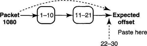
Figure 9.10 maintains the same sorted list as in Figure 9.9 but also keeps a pointer to the end of the list. Optimizing for the case that fragments arrive in order and are nonoverlapping, when a fragment containing bytes 22–30 arrives, the implementation checks the ending byte number of the last received fragment (stored in a register, equal to 21) against the start offset of the new fragment. Since 22 is 21 + 1, all is well. The new end byte is updated to the end byte of the new fragment (30), and the pointer is updated to point to the newly arrived fragment after linking it at the end of the list. Finally, if the newly arriving fragment is a last fragment, reassembly is done.
Compared to the implementation in Figure 9.9, the check for completion as well as the check to find out where to place a fragment takes constant and not linear time. Similarly, one can cache the expected packet ID (as in the TCP or UDP PCB lookup implementations) to avoid a list traversal when searching for the fragment list. Finally, using data structures such as pbufs instead of mbufs, even the need for an extra copy can be avoided by directly copying a received fragment into the buffer at the appropriate offset.
If the expected case fails, the implementation can revert to the standard BSD processing. For example, Chandranmenon and Varghese [CV98a], which describe this expected-case optimization in which the code keeps two lists and directly reuses the existing BSD code (which is hard to get right!) when the expected case fails. The expected case is reported by Chandranmenon and Varghese [CV98a] as taking 38 SPARC instructions, which is comparable with Jacobson’s TCP estimates.
As with header prediction, it is worth applying Caveat Q8 and examining the sensitivity of this optimization of this implementation to the assumptions. Actually, it turns out to be pretty bad. This is because measurements indicate that many recent implementations, including Linux, have senders send out fragments in reverse order! Thus fragments arrive in reverse order 9% of the time [SMC01].
This seemingly eccentric behavior is justified by the fact that it is only the last fragment that carries the length of the entire packet; by sending it first the sender allows the receiver to know what length buffer to allocate after the first fragment is received, assuming the fragments arrive in FIFO order. Note that the FIFO assumption still holds true. However, Figure 9.10 has a concealed but subtle additional assumption: that fragments will be sent in offset order. Before reading further, think how you might modify the implementation of Figure 9.10 to handle this case.
The solution, of course, is to use the first fragment to decide which of two expected cases to optimize for. If the first fragment is the first fragment (offset 0), then the implementation uses the mode described in Figure 9.10. If the first fragment is the last (last bit set), the implementation jumps to a different state, where it expects fragments in reverse order. This is just the dual of Figure 9.10, where the next fragment should have its last byte number to be 1 less (as opposed to 1 more) than the start offset of the previous fragment. Similarly, the next fragment is expected to be pasted at the start of the list and not the end.
9.5 CONCLUSIONS
This chapter describes techniques for efficient buffer allocation, CRC and checksum calculation, protocol processing such as TCP, and finally reassembly.
For buffer allocation, techniques such as the use of segregated pools and batch allocation promise fast allocation with potential trade-offs: the lack of storage efficiency (for segregated pools) versus the difficulty of coalescing noncontiguous holes (for batch allocation). Buffer sharing is important to use memory efficiently and can be done by efficiently stealing buffers from large users or by using dynamic thresholds.
For CRC calculation, efficient multibit remainder calculation finesses the obvious waste (P1) of calculating CRCs one bit at a time, even using LFSR implementations. For checksum calculation, the main trick is to fit the computation to the underlying machine architecture, using large word lengths, lazy checks for carries, and even parallelism. The optimizations for TCP, UDP, and reassembly are all based on optimizing simple expected cases (e.g., FIFO receipt, no errors) that cut through a welter of corner cases that the protocol must check for but rarely occur. Figure 9.1 presents a summary of the techniques used in this chapter together with the major principles involved.
Beyond the specific techniques, there are some general lessons to be gleaned. First, when considering the buffer-stealing algorithm, it is tempting to believe that finding the user with the largest buffer allocation requires a heap, which requires logarithmic time. However, as with timing wheels in Chapter 7, Mckenney’s algorithm exploits the special case that buffer sizes only increase and decrease by 1.
The general lesson is that for algorithmics, special cases matter. Theoreticians know this well; for example, the general problem of finding a Hamiltonian cycle [CLR90] is hard for general graphs but is trivial if the graph is a ring. In fact, the practitioner of algorithmics should look for opportunities to change the system to permit special cases that permit efficient algorithms.
Second, the dynamic threshold scheme shows how important it is to optimize one’s degrees of freedom (P13), especially when considering dynamic instead of static values for parameters. This is a very common evolutionary path in many protocols: for example, collision-avoidance protocols evolved from using fixed backoff times to using dynamic backoff times in Ethernet; transport protocols evolved from using fixed window sizes to using dynamic window sizes to adjust to congestion; finally, the dynamic threshold scheme of this chapter shows the power of allowing dynamic buffer thresholds.
Third, the discussion of techniques for buffer sharing shows why algorithmics — at least in terms of abstracting common networking tasks and understanding a wide spectrum of solutions for these tasks — can be useful. For example, when writing this chapter it became clear that buffer sharing is also part of many credit-based protocols, such as Ozveren et al. [OSV94] (see the protocol in Chapter 15) — except that in such settings a sender is allocating buffer space at a distant receiver. Isolating the abstract problem is helpful because it shows, for instance, that the dynamic threshold scheme of Choudhury and Hahne can provide finer grain buffer sharing than the technique of Ozveren et al. [OSV94].
Finally, the last lesson from header prediction and fast reassembly is that attempts to design new protocols for faster implementation can often be countered by simpler implementations. In particular, arguing that a protocol is “complex” is often irrelevant if the complexities can be finessed in the expected case.
As a second example, a transport protocol [SN89] was designed to allow efficient sequence number processing for protocols that used large windows and could handle out-of-order delivery. The protocol embedded concepts such as chunks of contiguous sequence numbers into the protocol for this purpose. Simple implementation tricks described in the patent [TVHS92] can achieve much the same effect, using large words to effectively represent chunks without redesigning the protocol.
Thus history teaches that attempts to redesign protocols for efficiency (as opposed to more functionality) should be viewed with some scepticism.
9.6 EXERCISES
1. Dynamic Buffer Thresholds and Credit-Based Flow Control: Read the credit-based protocol described in Chapter 15. Consider how to modify the buffer-sharing protocol of Chapter 15 to use dynamic thresholds. What are some of the possible benefits? This last question is ideally answered by a simulation, which would make it a longer-term class project.
2. Incremental Checksum Computation: RFC 1141 states that when an IP header with checksum H is modified by changing some 16-bit field value (such as the TTL field) m to a new value m′, then the new checksum should become H + m + m′, where X denotes the 1’s complement of X. While this works most of the time, the right equation, described in RFC 1624, is to compute (H + m + m’): This is slightly more inefficient but correct. This should show that tinkering with the computation can be tricky and requires proofs.
To see the difference between these two implementations, consider an example given in RFC 1624 with an IP header in which a 16-bit field m = 0x5555 changes to m′ = 0x3285. The 1’s-complement sum of all the remaining header bytes is 0xCD7A. Compute the checksum both ways and show that they produce different results. Given that these two results are really the same in 1’s complement notation (different representations of zero), why might it cause trouble at the receiver?
3. Parallel Checksum Computation: Figure out how to modify checksum calculation in hardware so as to work on W chunks of the packet in parallel and finally to fold all the results.
4. Hardware Reassembly: Suppose the FIFO assumption is not true and fragments arrive out of order. In this problem your assignment is to design an efficient hardware reassembly scheme for IP fragments subject to the restrictions stated in Chapter 2. One idea you could exploit is to have the hardware DMA engine that writes the fragment to a buffer also write a control bit for every word written to memory. This only adds a bit for every 32 bits.
When all the fragments have arrived, all the bits are set. You could determine whether all bits are set by using a summary tree, in which all the bits are leaves and each node has 32 children. A node’s bit is set if all its children’s bits are set. The summary tree does not require any pointers because all node bit positions can be calculated from child bit positions, as in a heap. Describe the algorithms to update the summary tree when a new fragment arrives. Consider hardware alternatives in which packets are stored in DRAM and bitmaps are stored in SRAM, as well as other creative possibilities.