3.18.3.1 Distance based triangulation

Denote to be the Euclidean distance between the position of the nth sensor and the (unknown) source location r, namely, . may be estimated from the sensor observations for certain type of sensors such as laser or infrared light. One may write down N quadratic equations:

(18.2)

Subtracting both sides of each pair of successive equations above to eliminate the unknown term , it leads to linear equations

(18.3)

These linear systems of equations may be expressed in a matrix form:

(18.4)

In general, the accuracy of the distance estimate may be compromised by estimation errors. Thus, a more realistic model should include an estimation noise term:

(18.5)

where e is a zero-mean, uncorrelated random noise vector such that

Then r may be estimated using weighted least square method that seeks to minimize a cost function

The leads to

(18.6)

3.18.3.2 Angle based triangulation

Denote to be incidence angle from the source into the nth sensor using the north direction as the reference direction. We further assume that the angle is positive along the clock-wise direction. Referring to Figure 18.1, it is easily verified that

(18.7)

Rearranging terms and collecting all N equations, one has

(18.8)

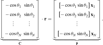
Or, in matrix formation:

(18.9)

Similar to Eq. (18.5), the observation p may be contaminated with noise. As such, the source location may be obtained via a weighted least square estimate. For the sake of notation simplicity, one may use e to denote the noise vector as in Eq. (18.5). Then, the weighted least square estimation of r becomes:

(18.10)

3.18.3.3 Triangulation: generalizations

In Sections 3.18.3.1 and 3.18.3.2, single target triangulation localization algorithms for distance measurements and incidence angle measurements have been discussed. Both of these situations lead to an over-determined linear systems of Eqs. (18.5) and (18.9). Therefore, when both distance measurements and incidence angle measurements are available, these two equations may be combined and solved jointly.

When there are two or more sources (targets), a number of issues will need to be addressed. First of all, when a sensor receives signals emitted from two or more sources simultaneously, it may not be able to distinguish one signal from another if these signals overlap in time, space and frequency domains. This is the traditional signal (source) separation problem[20–23]. Secondly, even individual sources may be separated by individual sensors, which of the signals received by different sensors correspond to the same source is not always easy to tell. This is the so called data association problem [24,25]. A comprehensive survey of these two issues is beyond the scope of this chapter.

As discussed earlier, while localization may be accomplished via triangulation, the measurements of sensor to source distance or source to sensor incidence angle must be estimated based on received signals. The mathematical model of the received source signals, known as the signal propagation model will be surveyed in the next section.

Attenuation: The amplitude of the source signal often attenuates rapidly as source to sensor distance increases. Hence, examining relative attenuation of signal strength provides an indirect way to estimate source to sensor distance. For a point source, the rate of attenuation is often inversely proportional to . The communication channel between the sensor and the source may also be frequency selective such that the attenuation rates are different from different frequency bands. For example, high frequency sound often attenuate much faster than low frequency sound. Thus the amplitude waveform as well as the energy of the source signal at the sensor may be distorted. If the signal propagation is subject to multi-path distortion, the attenuation rate may also be affected. Yet another factor that affects the measured amplitude of received signal is the sensor gain. Before the received analog signal is to be digitized, its magnitude will be amplified with adaptive gain control to ensure the dynamic range of the analog-to-digital converter (ADC) is not saturated. Furthermore, the signal strength attenuation may not be uniform over all directions, and the point source assumption may not be valid at short distance.

Time delay: Denote to be the signal propagation speed in the corresponding medium, the time for the source signal traveling to the sensor can be evaluated as

(18.12)

However, the time delay due to signal propagation may be impacted by non-homogeneous mediums. The consequence may be refraction or deflection of signal propagation and the accuracy of time delay estimation may be compromised.

Phase distortion: The nonlinear phase distortion due to frequency selective channel property may also distort the morphology of the signal waveform, making it difficult to estimate any phase difference between received signals at different sensors.

Noise: While the source signal travels to each sensor, it may suffer from (additive) channel noise or interferences by other sources. It is often assumed that the background noise observed at each sensor is a zero-mean, un-correlated, and wide-sense stationary random process, having Gaussian distribution. Moreover, the background noise processes at different sensors are assumed to be statistically independent to each other. Such assumptions may need to be modified for situations when the background noise also include high energy impulsive noise or interferences.

3.18.4.0.1 Received signal strength indicator (RSSI)

A popular simplified model concerns only amplitude attenuation:

(18.14)

Here the propagation delay, phase distortion, and noise are all ignored. Instead, is used to denote the sensor gain of the nth sensor. Thus, one may write

(18.15)

Averaging over a short time interval centered at the sampling time t, one may express the energy of the received signal during this short period as

(18.16)

where is the received signal energy at time t at sensor , and

It is assumed that the K source signals are statistically, mutually independent, such that

Moreover, the background noise is also independent to the signal, besides being . random variables such that

and

(18.17)

Here is a random variable with a distribution. However, as discussed in [19], for practical purposes, can be modeled as a Gaussian random variable with a positive mean value and variance .

Equations (18.15) or (18.16) are often used in source localization algorithms that are based on Received Signal Strength Indicator (RSSI) [26,27] to infer the target location.

3.18.4.1 Time delay estimation

Time delay estimation [28,29] has a long history of signal processing applications [30–32]. It is assumed that

(18.18)

If can be estimated accurately, the source to sensor distance may be estimated using Eq. (18.12). Thus, the key issue is to estimate .

If the original source signal and the received signal are both available, then the time delay may be estimated using a number of approaches.

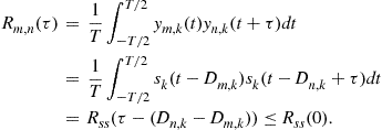
Assume and are both zero-mean white sense stationary random processes over a time interval , the cross-correlation between them is defined as

(18.19)

Substituting in Eq. (18.18) into Eq. (18.19), and assume if and otherwise, one has

(18.20)

Therefore, a maximum likelihood estimate of the time delay will be

(18.21)

There is a fundamental difficulty in applying Eq. (18.21) to estimate source to sensor signal propagation delay: may not be available at the sensor. This is often the case when the source is non-cooperative such as an intruder. On the other hand, if the source is cooperative, it may transmit a signal that consists of a time stamp. If the clocks at the sensor and at the source are synchronized as in the case of the global positioning system (GPS) [1], the sensor can compare the receiving time stamp against the sending time stamp and deduce the transit time without using cross correlation.

In some applications, the direction of the source is known but the distance between the source and the sensor is to be measured. Then, a round trip signal propagation delay may be estimated using cross-correlation method by emitting a signal from the sensor toward the source and bounding back to the sensor. Then, both the transmitted signal and received signal will be available at the sensor and above cross-correlation method may be applied to estimate the source to sensor distance.

In general, when is unavailable at the sensor, a difference of time of arrival from the same source at different sensors will allow one to estimate the incidence angle of source signal. This is the Time Difference of Arrival (TDoA) feature mentioned in literatures [33,34]. With TDoA, a Generalized Cross Correlation (GCC) [28] may be applied to estimate .

Ideally, one would hope and . As such, one computes the cross correlation

(18.22)

Thus,

(18.23)

With the presence of channel noise and channel model , Knapp and Carter [28] proposed to pre-filter and to improve the accuracy of the TDOA estimate by enhancing the signal to noise ratio (SNR) of estimate. Specifically, denote and respectively as the Fourier transform of the received signal and , and also denote and respectively as the spectrum of the pre-filters for and , the GCC is defined as:

(18.24)

Once is estimated, one has the following relation:

(18.25)

Hence TDOA provides a relative distance measure from the source to two different sensors. We note by passing that Eq. (18.25) defines a parabolic trajectory for potential target location r.

3.18.4.2 Angle of arrival estimation

For narrow band source signal, if sensors are fully synchronized, phase difference between received sensor signals may be used to estimate the incidence angle of source signal.

Assume a point source emitting a narrow band (single harmonic) signal described in Eq. (18.11). Under a far field assumption, that is

(18.26)

the waveform of the source signal can be modeled as a plane wave such that the incidence angle of the source to each of the sensor nodes will be identical. This makes it easier to represent the time difference of arrival as a steering vector which is a function of the incidence angle and the sensor array geometry.

Again, let north be a reference direction of the incidence angle which increases along the clock-wise direction. Then a unit vector along the incidence angle can be expressed as . The time difference of arrival between sensor nodes m and N can be expressed as:

(18.27)

Substitute the expression of a narrow band signal as shown in Eq. (18.11) into the expression of received signal described in Eq. (18.18), one has

(18.28)

where is the frequency response of evaluated at and is independent of , and under the far field assumption Eq. (18.26). Assume , then the received signal of all N sensors may be represented by

(18.29)

where

is a steering vector with respect to a narrow band source with incidence angle using the signal received at the Nth sensor as a reference. It represents the phase difference of the received sensor signals with respect to a plane wave traveling at an incidence angle . With K narrow band sources, the received signal vector than may be expressed as:

(18.30)

where

and

Equation (18.30) is the basis of many array signal processing algorithms [3,35,36] such as MUSIC [37]. Specifically, the covariance matrix of may be decomposed into two parts:

(18.31)

where and are the signal and noise covariance matrix respectively. In particular, has a rank equal to K. In practice, one would estimate the covariance matrix from received signal and perform eigenvalue decomposition:

(18.32)

where are the largest K eigenvalues and columns of are corresponding eigenvectors. The K dimensional subspace spanned by columns of the matrix is called the signal subspace. On the other hand, are the remaining eigenvalues. The dimensional subspace spanned by columns of the matrix is called the noise subspace. Define

(18.33)

as a generic steering vector, the MUSIC method evaluates the function

(18.34)

This MUSIC spectrum then will show high peaks at .

3.18.5.1 Bayesian source localization based on RSSI

For convenience of discussion, let us rewrite Eq. (18.16) here after a linear transformation of the random variables

(18.35)

Then,

(18.36)

or in matrix notation

(18.37)

Since is a normalized Gaussian random vector with zero mean and identity matrix as its covariance, the likelihood function that z is observed at N sensors, given the K source signal energy and source locations can be expressed as:

(18.38)

A maximum likelihood (ML) estimate of may be obtained by maximizing L or equivalently, minimizing the negative log likelihood function

(18.39)

Setting the gradient of against equal to 0, one may express the estimate of the source signal energy vector as

(18.40)

where is the pseudo inverse of the H matrix. Substituting Eq. (18.40) into Eq. (18.39), one has

(18.41)

Equation (18.41) is significant in several ways: (a) The number of unknown parameters is reduced from to assuming that the dimension of is 2. (b) To minimize , the source locations should be chosen such that the (normalized) energy vector z falls within the subspace spanned by columns of the H matrix as close as possible. In [19], this property is leveraged to derive a multi-resolution projection method for solving the source locations.

In deriving the ML estimates of source locations, no prior information about source locations is used. If, as in a tracking scenario, the prior probability of source locations, is available, then the a posterior probability may be expressed as:

(18.42)

Maximizing above expression then will lead to the Bayesian estimate of the source locations and corresponding source emitted energies during .

3.18.5.2 Non-linear least square source localization using RSSI

Assume a scenario of a single source (). If one ignores the noise energy term, Eq. (18.16) can be expressed as (using notation in Eq. (18.35))

(18.43)

Based on this approximated distance, the source location r and the source energy S may be estimated.

3.18.5.3 Source localization using time difference of arrival

Denote

(18.49)

Substituting Eq. (18.49) into Eq. (18.25) with , one has

(18.50)

Squaring both sides of above equation for both indices m and n,

Subtracting both sides of above equations, it yields (for )

Restricting , one may express above into a matrix format:

(18.51)

The source location r may be solved from above equation using least square estimate subject to the constraint quadratic equality constraint according to Eq. (18.49):

(18.52)

3.18.5.4 Source localization using angle of arrival

When there is only a single source in the sensing field, the angle based triangulation method discussed in Section 3.18.3.2 can be applied to estimate the source location. With more than one sources, a data correspondence problem must be resolved. Such a problem has been addressed in terms of N-Ocular stereo[38].

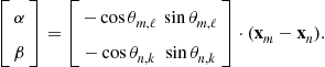
Assume that each of the nth sensor detects K distinct incidence angles from the K sources. Thus, there are incidence angles . If at the nth sensor, it receives a source signal with incidence angle , then the source location may be expressed as

(18.53)

Similarly, for the mth sensor, for the th incidence angle, the source location is at

Therefore, if these two sources are the same source (e.g., ), then one must have a valid solution, namely, , and to the following linear system of equations:

(18.54)

The solution can be represented expressively as:

(18.55)

If both and are positive, then is a potential source location. Since it is derived from observation of two sensors, it is called a bi-ocular solution. Otherwise, the solution will be discarded. Substituting the pairs angles into Eq. (18.55), one may obtain up to valid solutions which are candidates for the K possible source locations, assuming there is no occlusion. The collection of these solutions will be denoted by indicating they are consistent with two sensor observations.

Now for a third sensor at with incidence angles , one may test if any of the potential solutions in , lies in any of the K incidence rays originated from . This is easily accomplished by evaluating

(18.56)

If the resulting , then the candidate solution r will be promoted into a tri-ocular solution set for being consistent with 3 sensor observations. Repeat above procedure until is obtained or when the size of the solution set reduces to K. Then the procedure is terminated and the K source positions are obtained.

Two issues will need to be addressed when applying above procedures: (a) A false matching solution may be obtained where many incidence rays intersect but no source exists. Fortunately, each incidence ray passing through a false matching position should have two or more matching points. Thus, a false matching solution may be identified if every incidence rays passing through it have more than one matching point. (b) The azimuth incidence angle estimates may be inaccurate. Hence the intersections may not coincide at the same position. Several remedies of this problem have been discussed in [38]. In practice, one may partition the sensing field into mesh grids whose size roughly equal to the angle estimation accuracy. The position of a potential N-ocular solution then will be registered with the corresponding mesh grid rather than a specific point. A mesh grid will be included into if there are m intersections fall within its range.

3.18.6.1 Dynamic and observation models

Statistically, tracking is modeled as a sequential Bayesian estimation problem of a dynamic system whose states obey a Markov model. In the context of source localization and tracking, the dynamic system that describes a single target moving in a 2D plane has the form

(18.57)

where is the time duration between t and , and is a zero mean Gaussian random number with variance which models the acceleration.

Signal received at N sensors as a function of source location and source signal gives the observation model. Examples of observation model include Eqs. (18.15) and (18.18). These nonlinear models may be expressed as:

(18.58)

where the observation noise is a zero mean Gaussian random variable with variance . Sometimes, intermediate observation model, such as sensor to source distance estimate Eq. (18.12), Eq. (18.25), or source signal incidence angle estimate such as Eq. (18.53).

In general, the sensor observation , or the intermediate measurements are highly nonlinear equations of the source position and speed . Alternatively, one may apply methods discussed in this chapter to estimate based only on current observation , and express a derived observation equation as:

(18.59)

3.18.6.2 Sequential Bayesian estimation

The state transition described in Eqs. (18.57) and (18.58) can be described by a Markov chain model such that

and

As such, it is easily verified that

(18.60)

Denote to be the observations up to time t, and to be the conditional probability of given . Given the state estimation (location and speed of the source) at previous time step , the dynamic model Eq. (18.57) allows the prediction of the location and speed of the source at time t:

(18.61)

where

(18.62)

has a normal distribution. Similarly,

(18.63)

Applying Bayesian rule, one has

(18.64)

3.18.6.3 Kalman filter

Based on the sequential Bayesian formulation, one may deduce the well-known Kalman filter for the linear observation model (Eq. (18.59)). Specifically, the Kalman filter computes the mean and covariance matrix of the probability distribution

where

See Vol. 1, Chapter 2, Continuous-Time Signals and Systems

See Vol. 1, Chapter 3, Discrete-Time Signals and Systems

See Vol. 1, Chapter 4, Random Signals and Stochastic Processes

See Vol. 1, Chapter 11, Parametric Estimation

See Vol. 1, Chapter 19 A Tutorial Introduction to Monte Carlo Methods

See this volume, Chapter 5, Distributed Signal Detection

See this volume, Chapter 7, Geolocation—Maps, Measurements, Models, and Methods

See this volume, Chapter 19, Array Processing in the Face of Nonidealities

References

1. Daly P. Electron Commun Eng J. 1993;5:349–357.
2. Parkinson BW, Spilker JJ, eds. Global Positioning System: Theory and Applications. vol. 1. American Institute of Astronautics and Aeronautics 1996.
3. Owsley NL. In: Haykin S, ed. Array Signal Processing. Englewood-Cliffs, NJ: Prentice-Hall; 1991.
4. Zhou S, Willett P. IEEE Trans Signal Process. 2007;55:3104–3115.
5. Valin P, Jouan A, Bosse E. In: Bellingham, WA, USA, Orlando, FL, USA: Society of Photo-Optical Instrumentation Engineers; 1999;126–138. Proc SPIE-1999 Sensor Fusion: Architectures, Algorithms, and Applications III. vol. 3719.
6. Duckworth GL, Frey ML, Remer CE, Ritter S, Vidaver G. In: The International Society for Optical Engineering 1995;16–29. Proc SPIE. vol. 2344.
7. Friedrich C, Wegler U. Geophys Res Lett. 2005;32:L14312.
8. Gajewski D, Sommer K, Vanelle C, Patzig R. Geophysics. 2009;74:WB55–WB61.
9. J. Zhao, Seismic signal processing for near-field source localization, Ph.D. Dissertation, University of California, Los Angeles, 2007.
10. Ramirez RR. Scholarpedia. 2008;3(11):1073.
11. B.C. Basu, S.A. Pentland, in: Proceedings of ICASSP’01, vol. 5, pp. 3361–3364.
12. Aarabi P, Mahdavi A. In: Proceedings of ICASSP’02. IEEE 2002;273–276.
13. Chen JC, Yao K, Hudson RE. IEEE Signal Process Mag. 2002;19:30–39.
14. Chen J, Hudson RE, Yao K. IEEE Trans Signal Process. 2002;50:1843–1854.
15. Hu YH, Sheng X, Li D. In: IEEE Workshop on Multimedia Signal Processing. St. Thomas, Virgin Island: IEEE; 2002.
16. Li D, Hu YH. EURASIP J Appl Signal Process. 2003;321–337.
17. Sheng X, Hu YH. In: Proceedings of the International Symposisum on Information Processing in Sensor Networks (IPSN’03). Palo Alto, CA: Springer-Verlag; 2003;285–300.
18. Sheng X, Hu YH. In: Montreal, Canada: IEEE; 2004;972–975. Proceedings of ICASSP’04. vol. 3.
19. Sheng X, Hu YH. IEEE Trans Signal Process. 2005;53:44–53.
20. Amari S, Cichocki A, Yang HH. In: Proceedings of Advances in Neural Information Processing Systems (NIPS’96). MIT Press 1996;757–763.
21. Cardoso JF. Proc IEEE. 1998;86:2009–2025.
22. Douglas SC. In: Hu YH, Hwang JN, eds. Handbook of Neural Network Signal Processing. Boca Raton, FL: CRC Press; 2001; Chapter 7.
23. Gelle G, Colas M, Delaunay G. Mech Syst Signal Process. 2000;14:427–442.
24. Chang K-C, Chong C-Y, Bar-Shalom Y. IEEE Trans Automatic Control. 1986;31:889–897.
25. M. Ito, S. Tsujimichi, Y. Kosuge, in: Proceedings of the International Conference on Industrial Electronics, Control and Instrumentation, New Orleans, LA, vol. 3, pp. 1260–1264.
26. Savarese C, Rabaey JM, Beutel J. In: Proceedings of ICASSP’2001. Salt Lake City, UT: IEEE; 2001;2676–2679.
27. Seshadri V, Zaruba G, Huber MA. In: Proceedings of the International Conference on Pervasive Computing and Communications (PerCom’05). IEEE 2005;75–84.
28. Knapp CH, Carter GC. IEEE Trans Acoust Speech Signal Process. 1976;24:320–327.
29. Carter GC, ed. Coherence and Time Delay Estimation. IEEE Press 1993.
30. Chan YT, Hattin RV, Plant JB. IEEE Trans Acoust Speech Signal Process. 1978;26:217–222.
31. Tung TL, Yao K, Reed CW, Hudson RE, Chen D, Chen JC. In: The International Society for Optical Engineering 1999;220–233. Proceedings of SPIE. vol. 3807.
32. Benesty J, Chen J, Huang Y. IEEE Trans Speech Audio Process. 2004;1542:509–519.
33. Gustafsson F, Gunnarsson F. In: IEEE 2003;553–556. Proceedings of ICASSP’03. vol. 6.
34. Yang L, Ho KC. IEEE Trans Signal Process. 2009;57:4598–4615.
35. Krim H, Viberg M. IEEE Signal Process Mag. 1996;1583:67–94.
36. Tuncer E, Friedlander B, eds. Classical and Modern Direction-of-Arrival Estimation. Academic Press 2010.
37. Stoica P, Nehorai A. IEEE Trans, Acoust Speech Signal Process. 1989;37:720–741.
38. Sogo T, Ishiguro H, Trivedi MM. In: Proceedings of IEEE Workshop Omnidirectional Vision. IEEE 2000;153–160.
39. Julier SJ, Uhlmann JK. Proc IEEE. 2004;92:401–422.
40. Arulampalam M, Maskell S, Gordon N, Clapp T. IEEE Trans Signal Process. 2002;50:174–188.
41. Sheng X, Hu YH. In: Proceedings of 4th International Symposium on Information Processing in Sensor Networks (IPSN ’05). Los Angeles, CA: IEEE; 2005.