
Applications of Array Signal Processing
A. Lee Swindlehurst*, Brian D. Jeffs†, Gonzalo Seco-Granados‡ and Jian Li§, *Department of Electrical Engineering and Computer Science, University of California, Irvine, CA, USA, †Department of Electrical and Computer Engineering, Brigham Young University, Provo, UT, USA, ‡Department of Telecommunications and Systems Engineering, Universitat Autònoma de Barcelona, Bellaterra, Barcelona, Spain, §Department of Electrical and Computer Engineering, University of Florida, Gainesville, FL, USA, [email protected], [email protected], [email protected], [email protected]
Abstract
Array Signal Processing (ASP) refers to the collection and manipulation of data obtained from multiple spatially distributed sensors or antennas, in an effort to extract information about the sources of signals present in the data. As discussed in this chapter, such problems arise in many different fields, including radar, sonar, medicine, astronomy, communications, positioning, acoustics, etc. Typical ASP applications entail estimation of the source locations or extraction of source waveforms in the presence of strong interference and noise. A common mathematical model can be used to describe the data in most of these applications, a fact which has led to a significant cross-fertilization of ideas and algorithms that can be applied to ASP problems. The focus of this chapter is on describing many of the various ASP applications that have been studied in the literature, with a particular emphasis on explaining the assumptions made by researchers studying these problems and demonstrating how these assumptions lead to the common data model or something similar. Examples from radar, radio astronomy, sonar, biomedical imaging, acoustics and chemical sensors are given, and key references are provided for each topic to allow the reader to explore the applications in more detail.
Keywords
Array signal processing; Antenna arrays; Radar; Space-time adaptive processing; MIMO radar; Interference; Jamming; Clutter; Beamforming; Radio astronomy; Imaging; Array calibration; Spatial filtering; Global positioning system (GPS); Global navigation satellite system (GNSS); Positioning; Navigation; Direction-of-arrival (DOA) estimation; Direction finding; Long-term evolution (LTE); MIMO; Diversity; Spatial multiplexing; Equalization; Channel estimation; Space-time coding; Multi-user MIMO; WiMAX; Precoding; Ultrasound; Electroencephalography (EEG); Magnetoencephalography (MEG); Electrocorticography (ECoG); Sonar; Towed arrays; Radio frequency propagation; Acoustic propagation; Hydrophones; Microphones; Matched field processing; Acoustic vector sensors; Electromagnetic vector sensors; Microphone arrays; Source localization; Source separation; Chemical sensor arrays
3.20.1 Introduction and background
The principles behind obtaining information from measuring an acoustic or electro-magnetic field at different points in space have been understood for many years. Techniques for long-baseline optical interferometry were known in the mid-19th century, where widely separated telescopes were proposed for high-resolution astronomical imaging. The idea that direction finding can be performed with two acoustic sensors has been around at least as long as the physiology of human hearing has been understood. The mathematical duality observed between sampling a signal either uniformly in time or uniformly in space is ultimately just an elegant expression of Einstein’s theory of relativity. However, most of the technical advances in array signal processing have occurred in the last 30 years, with the development and proliferation of inexpensive and high-rate analog-to-digital (A/D) converters together with flexible and very powerful digital signal processors (DSPs). These devices have made the chore of collecting data from multiple sensors relatively easy, and helped give birth to the use of sensor arrays in many different areas.
Parallel to the advances in hardware that facilitated the construction of sensor array platforms were breakthroughs in the mathematical tools and models used to exploit sensor array data. Finite impulse response (FIR) filter design methods originally developed for time-domain applications were soon applied to uniform linear arrays in implementing digital beamformers. Powerful data-adaptive beamformers with constrained look directions were conceived and applied with great success in applications where the rejection of strong interference was required. Least-mean square (LMS) and recursive least-squares (RLS) time-adaptive techniques were developed for time-varying scenarios. So-called “blind” adaptive beamforming algorithms were devised that exploited known temporal properties of the desired signal rather than its direction-of-arrival (DOA).
For applications where a sensor array was to be used for locating a signal source, for example finding the source’s DOA, one of the key theoretical developments was the parametric vector-space formulation introduced by Schmidt and others in the 1980s. They popularized a vector space signal model with a parameterized array manifold that helped connect problems in array signal processing to advanced estimation theoretic tools such as Maximum Likelihood (ML), Minimum Mean-Square Estimation (MMSE) the Likelihood Ratio Test (LRT) and the Cramér-Rao Bound (CRB). With these tools, one could rigorously define the meaning of the term “optimal” and performance could be compared against theoretical bounds. Trade-offs between computation and performance led to the development of efficient algorithms that exploited certain types of array geometries. Later, concerns about the fidelity of array manifold models motivated researchers to study more robust designs and to focus on models that exploited properties of the received signals themselves.
The driving applications for many of the advances in array signal processing mentioned above have come from military problems involving radar and sonar. For obvious reasons, the military has great interest in the ability of multi-sensor surveillance systems to locate and track multiple “sources of interest” with high resolution. Furthermore, the potential to null co-channel interference through beamforming (or perhaps more precisely, “null-steering”) is a critical advantage gained by using multiple antennas for sensing and communication. The interference mitigation capabilities of antenna arrays and information theoretic analyses promising large capacity gains has given rise to a surge of applications for arrays in multi-input, multi-output (MIMO) wireless communications in the last 15 years. Essentially all current and planned cellular networks and wireless standards rely on the use of antenna arrays for extending range, minimizing transmit power, increasing throughput, and reducing interference. From peering to the edge of the universe with arrays of radio telescopes to probing the structure of the brain using electrode arrays for electroencephalography (EEG), many other applications have benefited from advances in array signal processing.
In this chapter, we explore some of the many applications in which array signal processing has proven to be useful. We place emphasis on the word “some” here, since our discussion will not be exhaustive. We will discuss several popular applications across a wide variety of disciplines to indicate the breadth of the field, rather than delve deeply into any one or try to list them all. Our emphasis will be on developing a data model for each application that falls within the common mathematical framework typically assumed in array processing problems. We will spend little time on algorithms, presuming that such material is covered elsewhere in this collection; algorithm issues will only be addressed when the model structure for a given application has unique implications on algorithm choice and implementation. Since radar and wireless communications problems are discussed in extensive detail elsewhere in the book, our discussion of these topics will be relatively brief.
3.20.2 Radar applications
We begin with the application area for which array signal processing has had the most long-lasting impact, dating back to at least World War II. Early radar surveillance systems, and even many still in use today, obtain high angular resolution by employing a radar dish that is mechanically steered in order to scan a region of interest. While such slow scanning speeds are suitable for weather or navigation purposes, they are less tolerable in military applications where split-second decisions must be made regarding targets (e.g., missiles) that may be moving at several thousand miles per hour. The advent of electronically scanned phased arrays addressed this problem, and ushered in the era of modern array signal processing.
Phased arrays are composed of from a few up to several thousand individual antennas laid out in a line, circle, rectangle or even randomly. Directionality is achieved by the process of beamforming: multiplying the output of each antenna by a complex weight with a properly designed phase (hence the term “phased” array), and then summing these weighted outputs together. The conventional “delay-and-sum” beamforming scheme involves choosing the weights to phase delay the individual antenna outputs such that signals from a chosen direction add constructively and those from other directions do not. Since the weights are applied electronically, they can be rapidly changed in order to focus the array in many different directions in a very short period of time. Modern phased arrays can scan an entire hemisphere of directions thousands of times per second. Figures 20.1 and 20.2 show examples of airborne and ground-based phased array radars.


Figure 20.2 The phased array used for targeting the Patriot surface-to-air missile system, composed of over 5000 individual elements.
For scanning phased arrays, a fixed set of beamforming weights is repeatedly applied to the antennas over and over again, in order to provide coverage of some area of interest. Techniques borrowed from time-domain filter design such as windowing or frequency sampling can be used to determine the beamformer weights, and the primary trade-off is beamwidth/resolution versus sidelobe levels. Adaptive weight design is required if interference or clutter must be mitigated. In principle, the phased array beamformer can be implemented with either analog or digital hardware, or a combination of both. For arrays with a very large number of antennas (e.g., the Patriot radar has in excess of 5000 elements), analog techniques are often employed due to the hardware and energy expense required in implementing a separate RF receive chain for each antenna. Hybrid implementations are also used in which analog beamforming over subsets of the array is used to create a smaller number of signal streams, which are then processed by a digital beamformer. This is a common approach, for example, in shipborne radar systems, where the targets of interest (e.g., low altitude cruise missiles) are typically located near the horizon. In such systems, analog beamforming with vertically-oriented strips of antennas are used to create a set of narrow azimuthal beams whose outputs can be flexibly combined using digital signal processing.
In this section, we will briefly discuss the two radar array applications that have received the most attention in the signal processing literature: space-time adaptive processing (STAP) and MIMO radar. Since these are discussed in detail elsewhere in the book, our discussion will not be comprehensive. While STAP and MIMO radar applications are typically used in active radar systems, arrays are also useful for passive radars, such as those employed in radio astronomy. We will devote a separate section to array signal processing for radio astronomy and discuss this application in much more detail, since it is not addressed elsewhere in the book.
3.20.2.1 Space-time adaptive processing
In many tactical military applications, airborne surveillance radars are tasked with providing location and tracking information about moving objects both on the ground and in the air. These radars typically use pulse-Doppler techniques since measuring the velocity of the objects of interest (or “targets”) is a key to accurately tracking them. As depicted in Figure 20.3, even when the targets are airborne, the transmit mainbeam and sidelobes will still illuminate the ground, especially when the radar look-direction is at a negative elevation angle (the targets may be below the radar platform). This means that the radar returns will contain significant energy from ground reflections, referred to as clutter. In addition, since pulse-Doppler techniques require an active radar, the frequency support of the radar signal is known, and an adversary can employ strong jamming to further mask the target returns. Often, the target signal is many tens of dB (e.g., 50 or more) weaker than the combination of jamming and clutter.

The difficulty of the situation is revealed by Figure 20.4, which shows the angle-Doppler power spectrum of data that contains a target together with clutter and jamming at a particular range. The jamming signal is due to a point source, so it is confined to a single arrival angle, but the jamming signal extends across the entire bandwidth of the data. The clutter energy lies on a ridge that cuts across the angle-Doppler space in a direction that is a function of the heading, altitude and velocity of the radar, and the current range bin of interest. Clutter in front of the radar will have a positive Doppler, and that behind it will be negative (as seen in Figure 20.3). Compared with the clutter and jamming, the target signal is weak and cannot be distinguished from the background due to the limited dynamic range of the receiver. Doppler filtering alone is not sufficient to reveal the target, since the jamming signal cuts across the entire bandwidth of the signal. On the other hand, using spatial filtering (beamforming) to null the jammer will still leave most of the clutter untouched. What is needed is a two-dimensional space-time filter. The process of designing and applying such a filter is referred to as space-time adaptive processing (STAP).

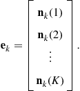
To better place STAP in the context of array signal processing problems, consider Figure 20.5 which depicts how data is organized in an M-antenna pulse-Doppler radar. The radar transmits a series of Kpulses separated in time by a fixed pulse repetition interval (PRI). In order to focus sufficient energy to obtain a measurable return from a target, the transmitted pulse is typically a very spatially focused signal steered towards a particular azimuth and elevation angle or look direction. However, the mathematical description of the STAP process can be described independently of this assumption. In between the pulses, the radar collects the returns from each of the M antennas, which are sampled after the received data is passed through a pulse-compression matched filter. Each sample corresponds to the aggregate contribution of scatterers (clutter and targets, if such exist) at a particular range together with any noise, jamming or other interference that may be present. The range for a given sample is given by the speed of light multiplied by half the time interval between transmission of the pulse and the sampling instant. Suppose we are interested in a particular range bin r. As shown in the figure, we will let
 (20.1)
![]() (20.2)
(20.2)
represent the ![]() vector of returns from the array after pulse t and the
vector of returns from the array after pulse t and the ![]() matrix of returns from all K pulses for range bin r, respectively.
matrix of returns from all K pulses for range bin r, respectively.

Alternatively, as shown in Figure 20.6, the data can be viewed as forming a cube over M antennas, K pulses, and B total range bins. Each range bin corresponds to a different slice of the data cube. Data from adjacent range bins ![]() will be used to counter the effect of clutter and jamming in the range bin of interest, which we index with
will be used to counter the effect of clutter and jamming in the range bin of interest, which we index with ![]() . The time required to collect the data cube for a given look direction is referred to as a coherent processing interval (CPI). If the radar employs multiple look directions, a separate CPI is required for each. Assuming the target, clutter and jamming are stationary over different CPIs, data from these CPIs can be combined to perform target detection and localization. However, in our discussion here we will assume that data from only a single CPI is available to determine the presence or absence of a target in range bin r.
. The time required to collect the data cube for a given look direction is referred to as a coherent processing interval (CPI). If the radar employs multiple look directions, a separate CPI is required for each. Assuming the target, clutter and jamming are stationary over different CPIs, data from these CPIs can be combined to perform target detection and localization. However, in our discussion here we will assume that data from only a single CPI is available to determine the presence or absence of a target in range bin r.

If a target is present in the data set ![]() , then the received signal can be modeled as
, then the received signal can be modeled as
 (20.3)
where ![]() is the amplitude of the return from the ith scatterer (
is the amplitude of the return from the ith scatterer (![]() corresponds to the target),
corresponds to the target), ![]() are the azimuth and elevation angles of the ith scatterer,
are the azimuth and elevation angles of the ith scatterer, ![]() is the corresponding Doppler frequency,
is the corresponding Doppler frequency, ![]() is the response of the M-element receive array to a signal from direction
is the response of the M-element receive array to a signal from direction ![]() is the signal transmitted by the jth jammer,
is the signal transmitted by the jth jammer, ![]() denote the DOA of the jth jammer signal,
denote the DOA of the jth jammer signal, ![]() represents the number of distinct clutter sources,
represents the number of distinct clutter sources, ![]() the number of jammers, and
the number of jammers, and ![]() corresponds to any remaining background noise and interference. We have also defined
corresponds to any remaining background noise and interference. We have also defined ![]() to contain all received signals except that of the target. Note that the above model assumes the relative velocity of the radar and all scatterers is constant over the CPI, so that the Doppler effect can be described as a complex sinusoid.
to contain all received signals except that of the target. Note that the above model assumes the relative velocity of the radar and all scatterers is constant over the CPI, so that the Doppler effect can be described as a complex sinusoid.
Technically, the amplitude and Doppler terms ![]() and
and ![]() will also depend on the azimuth and elevation angles of the ith scatterer since the Doppler frequency is position-dependent and the strength of the return is a function of the transmit beampattern in addition to the intrinsic radar cross section (RCS) of the scatterer. This is clear from Figure 20.7, which shows the geometry of the airborne radar with respect a clutter patch on the ground at some range r. The Doppler frequency for the given clutter patch at azimuth
will also depend on the azimuth and elevation angles of the ith scatterer since the Doppler frequency is position-dependent and the strength of the return is a function of the transmit beampattern in addition to the intrinsic radar cross section (RCS) of the scatterer. This is clear from Figure 20.7, which shows the geometry of the airborne radar with respect a clutter patch on the ground at some range r. The Doppler frequency for the given clutter patch at azimuth ![]() and elevation
and elevation ![]() can be determined from the following equations:
can be determined from the following equations:
![]() (20.4)
(20.4)
![]() (20.5)
(20.5)
![]() (20.6)
(20.6)
where ![]() denotes the earth’s radius, H is the altitude of the radar, and
denotes the earth’s radius, H is the altitude of the radar, and ![]() is the angle between the velocity vector of the radar and the clutter patch. To simplify the notation, we have dropped the explicit dependence of
is the angle between the velocity vector of the radar and the clutter patch. To simplify the notation, we have dropped the explicit dependence of ![]() and
and ![]() on
on ![]() . While the highest Doppler frequencies obviously occur for small
. While the highest Doppler frequencies obviously occur for small ![]() (forward- or rear-looking radar), the fact that
(forward- or rear-looking radar), the fact that ![]() changes relatively slowly for small
changes relatively slowly for small ![]() compared with
compared with ![]() near
near ![]() means that the Doppler spread of the clutter for a forward- or rear-looking radar will be smaller than that for the side-looking case.
means that the Doppler spread of the clutter for a forward- or rear-looking radar will be smaller than that for the side-looking case.

Figure 20.7 Geometry for determining the Doppler frequency due to a ground clutter patch at range r.
Rather than working with the data matrix ![]() , for STAP it is convenient to vectorize the data as follows:
, for STAP it is convenient to vectorize the data as follows:
 (20.7)
where ![]() is defined similarly to
is defined similarly to ![]() for the clutter and jamming, and where
for the clutter and jamming, and where
![]() (20.8)
(20.8)
 (20.9)
The ![]() vector
vector ![]() is the space-time snapshot associated with the given range bin (r) of interest. To detect whether or not a target signal was present in
is the space-time snapshot associated with the given range bin (r) of interest. To detect whether or not a target signal was present in ![]() , one may be tempted to use a minimum-variance distortionless response (MVDR) space-time filter of the form
, one may be tempted to use a minimum-variance distortionless response (MVDR) space-time filter of the form
 (20.10)
apply it to ![]() for various choices of
for various choices of ![]() , which then should lead to a peak in the filter output when
, which then should lead to a peak in the filter output when ![]() corresponds to the parameters of the target. The problem with this approach is that we will not have enough data available to estimate the covariance
corresponds to the parameters of the target. The problem with this approach is that we will not have enough data available to estimate the covariance ![]() ; if the target signal is only present in this range bin, then with a single CPI we only have a single snapshot that possesses this covariance.
; if the target signal is only present in this range bin, then with a single CPI we only have a single snapshot that possesses this covariance.
Fortunately, an alternative approach exists, since it can be shown via the matrix inversion lemma (MIL) that the optimal MVDR space-time filter is proportional to another vector that can be more readily estimated:
![]() (20.11)
(20.11)
which depends on the covariance ![]() of the clutter and jamming. In particular, STAP relies on the assumption that the statistics of the clutter and jamming in range bins near the one in question are similar, and can be used to estimate
of the clutter and jamming. In particular, STAP relies on the assumption that the statistics of the clutter and jamming in range bins near the one in question are similar, and can be used to estimate ![]() . For example, let
. For example, let ![]() represent a set containing the indices of
represent a set containing the indices of ![]() target-free range bins near r (since the target signal may leak into range bins immediately adjacent to bin r, these are typically excluded), then a sample estimate of
target-free range bins near r (since the target signal may leak into range bins immediately adjacent to bin r, these are typically excluded), then a sample estimate of ![]() may be formed as
may be formed as
![]() (20.12)
(20.12)
where ![]() is the space-time snapshot from range bin k. The
is the space-time snapshot from range bin k. The ![]() samples that compose
samples that compose ![]() are referred to as secondary data vectors.
are referred to as secondary data vectors.
Implementation of the space-time filter in (20.11) using a covariance estimate such as (20.12) is referred to as the “fully adaptive” STAP algorithm. The number ![]() of secondary data vectors chosen to estimate
of secondary data vectors chosen to estimate ![]() is a critical parameter. If it is too small, a poor estimate will be obtained; if it is too large, then the assumption of statistical similarity may be strained. Another critical parameter is the rank of
is a critical parameter. If it is too small, a poor estimate will be obtained; if it is too large, then the assumption of statistical similarity may be strained. Another critical parameter is the rank of ![]() . While in theory
. While in theory ![]() may be full rank, in practice its effective rank
may be full rank, in practice its effective rank ![]() is typically much smaller than its dimension MK, since the clutter and jamming are usually orders of magnitude stronger than the background noise. According to Brennan’s rule [1], the value of
is typically much smaller than its dimension MK, since the clutter and jamming are usually orders of magnitude stronger than the background noise. According to Brennan’s rule [1], the value of ![]() for a uniform linear array is
for a uniform linear array is ![]() , where
, where ![]() is a factor that depends on the speed of the array platform and the pulse repetition frequency (PRF), and is usually between
is a factor that depends on the speed of the array platform and the pulse repetition frequency (PRF), and is usually between ![]() and
and ![]() . The rank of
. The rank of ![]() for non-linear array geometries will be greater, although no concise formula exists in the general case. Factors influencing the rank of
for non-linear array geometries will be greater, although no concise formula exists in the general case. Factors influencing the rank of ![]() include the beamwidth and sidelobes of the transmit pulse (narrower pulses and lower sidelobes mean smaller
include the beamwidth and sidelobes of the transmit pulse (narrower pulses and lower sidelobes mean smaller ![]() ), the presence of intrinsic clutter motion (e.g., leaves on trees in a forest) or clutter discretes (strong specular reflectors), and whether the radar is forward- or side-looking (the Doppler spread of the clutter and hence
), the presence of intrinsic clutter motion (e.g., leaves on trees in a forest) or clutter discretes (strong specular reflectors), and whether the radar is forward- or side-looking (the Doppler spread of the clutter and hence ![]() is much smaller in the forward-looking case).
is much smaller in the forward-looking case).
The rank of ![]() is important in determining the minimum value for
is important in determining the minimum value for ![]() required to form a sufficiently accurate sample estimate. A general rule of thumb is that the number of required samples is on the order of
required to form a sufficiently accurate sample estimate. A general rule of thumb is that the number of required samples is on the order of ![]() . Even when these many stationary secondary range bins are available,
. Even when these many stationary secondary range bins are available, ![]() may still be much smaller than MK, and
may still be much smaller than MK, and ![]() will not be invertible. In such situations, a common remedy is to employ a diagonal loading factor
will not be invertible. In such situations, a common remedy is to employ a diagonal loading factor ![]() , and use the MIL to simplify calculation of the inverse:
, and use the MIL to simplify calculation of the inverse:
![]() (20.13)
(20.13)
![]() (20.14)
(20.14)
Another approach is to use a pseudo-inverse based on principal components.
Still, the computation involved in implementing the fully adaptive STAP algorithm is often prohibitive. The dimension MK of ![]() is often in the hundreds, and computational costs add up quickly when one realizes the STAP filtering must be performed in multiple range bins for each look direction. Most of the STAP research in recent years has been aimed at reducing the computational load to more reasonable levels. Two main classes of approaches have been proposed: (1) partially adaptive STAP and (2) parametric modeling. In the partially adaptive approach, the dimensions of the space–time data slice are reduced by means of linear transformations in space or time or both:
is often in the hundreds, and computational costs add up quickly when one realizes the STAP filtering must be performed in multiple range bins for each look direction. Most of the STAP research in recent years has been aimed at reducing the computational load to more reasonable levels. Two main classes of approaches have been proposed: (1) partially adaptive STAP and (2) parametric modeling. In the partially adaptive approach, the dimensions of the space–time data slice are reduced by means of linear transformations in space or time or both:
![]() (20.15)
(20.15)
Techniques for choosing the transformation matrices include beamspace methods, Doppler binning, PRI staggering, etc. The classical moving target indicator (MTI) approach can be thought of as falling in this class of algorithms for the special case where ![]() is one-dimensional. The dimension reduction achieved by partially adaptive methods not only reduces the computational load, but it improves the numerical conditioning and decreases the required secondary sample support as well.
is one-dimensional. The dimension reduction achieved by partially adaptive methods not only reduces the computational load, but it improves the numerical conditioning and decreases the required secondary sample support as well.
The parametric approach is based on the observation that in (20.14), as ![]() , we have
, we have
![]() (20.16)
(20.16)
Thus, the effect of ![]() is to approximately project the space-time signal vector onto the space orthogonal to the clutter and jamming. While
is to approximately project the space-time signal vector onto the space orthogonal to the clutter and jamming. While ![]() could be used to define this subspace, a more efficient approach has been proposed based on vector autoregressive (VAR) filtering. To see this, note from (20.3) and (20.7) that the clutter and jamming vector
could be used to define this subspace, a more efficient approach has been proposed based on vector autoregressive (VAR) filtering. To see this, note from (20.3) and (20.7) that the clutter and jamming vector ![]() for range bin k over the full CPI can be partitioned into samples for each individual pulse within the CPI:
for range bin k over the full CPI can be partitioned into samples for each individual pulse within the CPI:
 (20.17)
The VAR approach assumes that the clutter and jamming obey the following model for each pulse t:
![]() (20.18)
(20.18)
where L is typically assumed to be small (e.g., less than 5–7) and each matrix ![]() is
is ![]() for some chosen value of
for some chosen value of ![]() . The matrix coefficients of the VAR can be estimated for example by solving a standard least-squares problem of the form
. The matrix coefficients of the VAR can be estimated for example by solving a standard least-squares problem of the form
 (20.19)
where
 (20.20)
and the constraint ![]() is used to prevent a trivial solution. The matrix
is used to prevent a trivial solution. The matrix ![]() will approximately span the subspace orthogonal to
will approximately span the subspace orthogonal to ![]() , and based on (20.16) a suitable space-time filter would be given by
, and based on (20.16) a suitable space-time filter would be given by
![]() (20.21)
(20.21)
where
![]() (20.22)
(20.22)
This approach is referred to as the space-time autoregressive (STAR) filter. An example of the performance of the STAR filter is given in Figure 20.8 for a case with ![]() and
and ![]() . These results are for the same data set that generated the unfiltered angle-Doppler spectrum in Figure 20.4. Note that the clutter and jamming have been removed, and the target is plainly visible. Similar results were obtained in this case with the fully adaptive STAP method with diagonal loading, but required a value of
. These results are for the same data set that generated the unfiltered angle-Doppler spectrum in Figure 20.4. Note that the clutter and jamming have been removed, and the target is plainly visible. Similar results were obtained in this case with the fully adaptive STAP method with diagonal loading, but required a value of ![]() near 60.
near 60.

3.20.2.2 MIMO radar
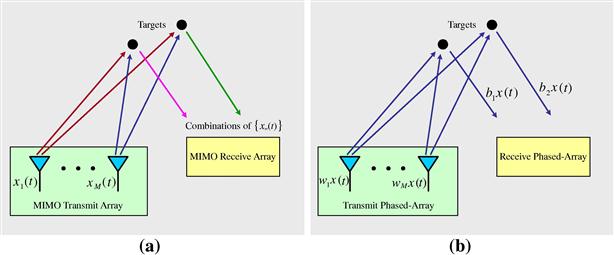
Multi-input multi-output (MIMO) radar is beginning to attract a significant amount of attention from researchers and practitioners alike due to its potential of advancing the state-of-the-art of modern radar. Unlike a standard phased-array radar, which transmits scaled versions of a single waveform, a MIMO radar system can transmit via its antennas multiple probing signals that may be chosen quite freely (see Figure 20.9). This waveform diversity enables superior capabilities compared with a standard phased-array radar. For example, the angular diversity offered by widely separated transmit/receive antenna elements can be exploited for enhanced target detection performance. For collocated transmit and receive antennas, the MIMO radar paradigm has been shown to offer many advantages including long virtual array aperture sizes and the ability to untangle multiple paths. Array signal processing plays critical roles in reaping the benefits afforded by the MIMO radar systems. In our discussion here, we focus on array signal processing for MIMO radar with collocated transmit and receive antennas.
An example of a UAV equipped with a MIMO radar system is shown in Figure 20.10, where the transmit array is sparse and the receive array is a filled (half-wavelength inter-element spacing) uniform linear array. When the transmit antennas transmit orthogonal waveforms, the virtual array of the radar system is a filled array with an aperture up to M times that of the receive array, where M is the number of transmit antennas. Many advantages of MIMO radar with collocated antennas result directly from this significantly increased virtual aperture size. For example, for small aerial vehicles (with medium or short range applications), a conventional phased-array system could be problematic since it usually weighs too much, consumes too much power, takes up too much space, and is too expensive. In contrast, MIMO radar offers the advantages of reduced complexity, power consumption, weight and cost by obviating phase shifts and affording significantly increased virtual aperture size.

Some typical examples of array processing in MIMO radar include transmit beampattern synthesis, transmit and receive array design, and adaptive array processing for diverse MIMO radar applications. We briefly describe these array processing examples in MIMO radar.
3.20.2.2.1 Flexible transmit beampattern synthesis
The probing waveforms transmitted by a MIMO radar system can be designed to approximate a desired transmit beampattern and also to minimize the cross-correlation of the signals reflected from various targets of interest—an operation that would hardly be possible for a phased-array radar.
The recently proposed techniques for transmit narrowband beampattern design have focused on the optimization of the covariance matrix ![]() of the waveforms. Instead of designing
of the waveforms. Instead of designing ![]() , we might think of directly designing the probing signals by optimizing a given performance measure with respect to the matrix
, we might think of directly designing the probing signals by optimizing a given performance measure with respect to the matrix ![]() of the signal waveforms. However, compared with optimizing the same performance measure with respect to the covariance matrix
of the signal waveforms. However, compared with optimizing the same performance measure with respect to the covariance matrix ![]() of the transmitted waveforms, optimizing directly with respect to
of the transmitted waveforms, optimizing directly with respect to ![]() is a more complicated problem. This is so because
is a more complicated problem. This is so because ![]() has more unknowns than
has more unknowns than ![]() and the dependence of various performance measures on
and the dependence of various performance measures on ![]() is more intricate than the dependence on
is more intricate than the dependence on ![]() .
.
There are several recent methods that can be used to efficiently compute an optimal covariance matrix ![]() , with respect to several performance metrics. One of the metrics consists of choosing
, with respect to several performance metrics. One of the metrics consists of choosing ![]() , under a uniform elemental power constraint (i.e., under the constraint that the diagonal elements of
, under a uniform elemental power constraint (i.e., under the constraint that the diagonal elements of ![]() are equal), to achieve the following goals:
are equal), to achieve the following goals:
a. Maximize the total spatial power at a number of given target locations, or more generally, match a desired transmit beampattern.
b. Minimize the cross-correlation between the probing signals at a number of given target locations.
Another beampattern design problem is to choose ![]() , under the uniform elemental power constraint, to achieve the following goals:
, under the uniform elemental power constraint, to achieve the following goals:
It can be shown that both design problems can be efficiently solved in polynomial time as a semi-definite quadratic program (SQP).
We comment in passing on the conventional phased-array beampattern design problem in which only the array weight vector can be adjusted and therefore all antennas transmit the same differently-scaled waveform. We can readily modify the MIMO beampattern designs for the case of phased-arrays by adding the constraint that the rank of ![]() is one. However, due to the rank-one constraint, both of these originally convex optimization problems become non-convex. The lack of convexity makes the rank-one constrained problems much harder to solve than the original convex optimization problems. Semi-definite relaxation (SDR) is often used to obtain approximate solutions to such rank-constrained optimization problems. The SDR is obtained by omitting the rank constraint. Hence, interestingly, the MIMO beampattern design problems are the SDRs of the corresponding phased-array beampattern design problems.
is one. However, due to the rank-one constraint, both of these originally convex optimization problems become non-convex. The lack of convexity makes the rank-one constrained problems much harder to solve than the original convex optimization problems. Semi-definite relaxation (SDR) is often used to obtain approximate solutions to such rank-constrained optimization problems. The SDR is obtained by omitting the rank constraint. Hence, interestingly, the MIMO beampattern design problems are the SDRs of the corresponding phased-array beampattern design problems.
We now provide a numerical example below, where we have used a Newton-like algorithm to solve the rank-one constrained design problems for phased-arrays. This algorithm uses SDR to obtain an initial solution, which is the exact solution to the corresponding MIMO beampattern design problem. Although the convergence of the said Newton-like algorithm is not guaranteed, we did not encounter any apparent problem in our numerical simulations.
Consider the beampattern design problem with ![]() transmit antennas. The main-beam is centered at
transmit antennas. The main-beam is centered at ![]() , with a 3 dB width equal to
, with a 3 dB width equal to ![]()
![]() . The sidelobe region is
. The sidelobe region is ![]() . The minimum-sidelobe beampattern design is shown in Figure 20.11a. Note that the peak sidelobe level achieved by the MIMO design is approximately 18 dB below the mainlobe peak level. Figure 20.11b shows the corresponding phased-array beampattern obtained by using the additional constraint
. The minimum-sidelobe beampattern design is shown in Figure 20.11a. Note that the peak sidelobe level achieved by the MIMO design is approximately 18 dB below the mainlobe peak level. Figure 20.11b shows the corresponding phased-array beampattern obtained by using the additional constraint ![]() . The phased-array design fails to provide a proper mainlobe (it suffers from peak splitting) and its peak sidelobe level is much higher than that of its MIMO counterpart. We note that, under the uniform elemental power constraint, the number of degrees of freedom (DOF) of the phased-array that can be used for beampattern design is equal to only
. The phased-array design fails to provide a proper mainlobe (it suffers from peak splitting) and its peak sidelobe level is much higher than that of its MIMO counterpart. We note that, under the uniform elemental power constraint, the number of degrees of freedom (DOF) of the phased-array that can be used for beampattern design is equal to only ![]() ; consequently, it is difficult for the phased-array to synthesize a proper beampattern. The MIMO design, on the other hand, can be used to achieve a much better beampattern due to its much larger number of DOF, viz.
; consequently, it is difficult for the phased-array to synthesize a proper beampattern. The MIMO design, on the other hand, can be used to achieve a much better beampattern due to its much larger number of DOF, viz. ![]() .
.

Figure 20.11 Minimum sidelobe beampattern designs, under the uniform elemental power constraint, when the 3 dB main-beam width is ![]() . (a) MIMO and (b) phased-array.
. (a) MIMO and (b) phased-array.
The radar waveforms are generally desired to possess constant modulus and excellent auto- and cross-correlation properties. Consequently, the probing waveforms can be synthesized in two stages: at the first stage, the covariance matrix ![]() of the transmitted waveforms is optimized, and at the second stage, a signal waveform matrix
of the transmitted waveforms is optimized, and at the second stage, a signal waveform matrix ![]() is determined whose covariance matrix is equal or close to the optimal
is determined whose covariance matrix is equal or close to the optimal ![]() , and which also satisfies some practically motivated constraints (such as constant modulus or low peak-to-average-power ratio (PAR) constraints). A cyclic algorithm for example, can be used for the synthesis of such an
, and which also satisfies some practically motivated constraints (such as constant modulus or low peak-to-average-power ratio (PAR) constraints). A cyclic algorithm for example, can be used for the synthesis of such an ![]() , where the synthesized waveforms are required to have good auto- and cross-correlation properties in time.
, where the synthesized waveforms are required to have good auto- and cross-correlation properties in time.
3.20.2.2.2 Array design
For a phased-array radar system, the transmission of coherent waveforms allows for a narrow mainbeam and, thus, a high signal-to-noise ratio (SNR) upon reception. When the locations of targets in a scene are unknown, phase shifts can be applied to the transmitting antennas to steer the focal beam across an angular region of interest. In contrast, MIMO radar systems, by transmitting different, possibly orthogonal waveforms, can be used to illuminate an extended angular region over a single processing interval, as we have demonstrated above.
Waveform diversity permits higher degrees of freedom, which enables the MIMO radar system to achieve increased flexibility for transmit beampattern design. The assumptions used in the discussions above are that the positions of the transmitting antennas, which also affect the shape of the beampattern, are fixed prior to the construction of ![]() followed by the synthesis of
followed by the synthesis of ![]() . At the receiver, sparse, or thinned, array design has been the subject of an abundance of literature during the last 50 years. The purpose of sparse array design has been to reduce the number of antennas (and thus reduce the cost) needed to produce desirable spatial receiving beampatterns. The ideas behind sparse receive array methodologies can be extended to that of sparse, MIMO array design. For example, cyclic algorithms can be used to approximate desired transmit and receive beampatterns via the design of sparse antenna arrays. These algorithms can be seen as extensions to iterative receive beampattern designs.
. At the receiver, sparse, or thinned, array design has been the subject of an abundance of literature during the last 50 years. The purpose of sparse array design has been to reduce the number of antennas (and thus reduce the cost) needed to produce desirable spatial receiving beampatterns. The ideas behind sparse receive array methodologies can be extended to that of sparse, MIMO array design. For example, cyclic algorithms can be used to approximate desired transmit and receive beampatterns via the design of sparse antenna arrays. These algorithms can be seen as extensions to iterative receive beampattern designs.
3.20.2.2.3 Adaptive array processing at radar receivers
Adaptive array processing plays a vital role at radar receivers, including those of MIMO radar. Conventional data-independent algorithms, such as the delay-and-sum approach for array processing, suffer from poor resolution and high sidelobe level problems. Data-adaptive algorithms, such as MVDR (Capon) receivers, have been widely used in radar receivers. These adaptive signal processing algorithms offer much higher resolution and lower sidelobe levels than the data-independent approaches. However, these algorithms can be sensitive to steering vector errors and also require a substantial number of snapshots to determine the second-order statistics (covariance matrices). To mitigate these problems, diagonal loading has been used extensively in practical applications to make adaptive algorithms feasible. However, too much diagonal loading makes the adaptive algorithm degenerate into data-independent methods, and the diagonal loading level may be hard to determine in practice. Parametric methods tend to be sensitive to data model errors and are not as widely used as the aforementioned data-adaptive algorithms.
In MIMO radar, adaptive array processing is essential, especially because many of the simple tricks used to achieve the longer virtual arrays, such as randomized antenna switching (also called randomized time-division multiple access (R-TDMA)) and slow-time code-division multiple access (ST-CDMA), provide sparse random sampling. Because of such sampling, the high sidelobe level problem suffered by data-independent approaches are exacerbated. Moreover, most of the radar signal processing problems encountered in practice do not have multiple snapshots. In fact, in most practical applications, only a single data measurement snapshot is available for adaptive signal processing. For example, in synthetic aperture radar (SAR) imaging, just a single phase history matrix is available for SAR image formation. Moreover the phase history matrix may not be uniformly sampled. In MIMO radar applications, including MIMO-radar-based space-time adaptive processing (STAP), synergistic MIMO SAR imaging and ground moving target indication (GMTI), and untangling multiple paths for diverse radar operations such as those encountered by MIMO over-the-horizon radar (OTHR), we essentially have just a single snapshot available at the radar receiver, especially in a heterogeneous clutter environment.
Fortunately, the recent advent of iterative adaptive algorithms, such as the iterative adaptive approach (IAA) and sparse learning via iterative minimization (SLIM), obviate the need of multiple snapshots and the uniform sampling requirements but retain desirable properties, including high resolution, low sidelobe level, and robustness against data model errors, of the conventional adaptive array processing methods. Moreover, for uniformly sampled data, various fast implementation strategies of these algorithms have been devised to exploit the Toeplitz matrix structures. These iterative adaptive algorithms are particularly suited for signal processing at radar receivers. They can also be used in diverse other applications, such as in sonar, radio astronomy, and channel estimation for underwater acoustic communications.
3.20.3 Radio astronomy
Radio astronomy is the study of our universe by passive observation of extra-terrestrial radio frequency emissions. Sources of interest for astronomers include (among others) radio galaxies, pulsars, supernova remnants, synchrotron radiation from excited material in a star’s magnetic field, ejection jets from black holes, narrowband emission and absorption lines from diffuse elemental or chemical compound matter that can be assayed by their characteristic spectral structure, and continuum thermal black body radiation emitted by objects ranging from stars to interstellar dust and gasses. The radio universe provides quite a different and complementary view to that which is visible to more familiar optical telescopes. Radio astronomy has enabled a much fuller understanding of the structure of our universe than would have been possible with visible light alone. With Doppler red shifting, the spectrum of interest ranges from as low as the shortwave regime near 10 MHz, to well over 100 GHz in the millimeter and submillimeter bands, and there are radio telescopes either in use or under development to cover much of this spectrum.
From the earliest days of radio astronomy, detecting faint deep space sources has pushed available technology to extreme performance limits. Early progress was driven by improvements in hardware with relatively straightforward signal processing and detection techniques. With the advent of large synthesis arrays, signal processing algorithms increased in sophistication. More recently, interest in phased array feeds (PAFs) has opened a new frontier for array signal processing algorithm development for radio astronomical observations.
Radio astronomy presents unique challenges as compared to typical applications in communications, radar, sonar, or remote sensing:
• Low SNR: Deep space signals are extremely faint. SNRs of ![]() are routine.
are routine.
• Radiometric detection: A basic observational mode in radio astronomy is “on-source minus off-source” radiometric detection where the source level is well below the noise floor and can only be seen by differencing with a noise only estimate. This requires stable power estimates of (i) system noise plus weak signal of interest (SOI) and (ii) noise power alone with the sensor steered off the SOI. The standard deviation of the noise power estimate determines the minimum detectable signal level, so that long integration times (minutes to hours) are required.
• Low system temperatures: With cryogenically cooled first stage low noise amplifiers, system noise temperatures can be as low as 15 K at L-band, including LNA noise, waveguide ohmic losses, downstream receiver noise, and spillover noise from warm ground observed beyond the rim of a dish reflector.
• Stability: System gain fluctuations increase the receiver output variance and place a limit on achievable sensitivity that cannot be overcome with increased integration time. High stability in gain, phase, noise, and beamshape response over hours is required to enable long term integrations to tease out detection of the weakest sources.
• Bandwidth: Some scientific observations require broad bandwidths of an octave or more. Digital processing over such large bandwidths poses serious computational burdens.
• Radio frequency interference (RFI): Observations in RFI environments outside protected frequency bands are common. Interference levels below the noise floor may be as problematic as strong interferers, since they are hard to identify and attenuate. Cancelation approaches also cause pattern rumble which limits sensitivity.
3.20.3.1 Synthesis imaging
Radio astronomical synthesis imaging uses interferometric techniques and some of the world’s largest sensor arrays to form high resolution images of the distribution of radio sources in deep space. Figure 20.12 presents two examples of the beautiful high resolution detail revealed by synthesis imaging from the Very Large Array (VLA) in New Mexico, and Figure 20.13 shows the VLA with its antennas configured in a compact central core configuration. The key to this technology is coherent cross-correlation processing (i.e., interferometry) of RF signals seen by pairs of widely separated antennas (up to 10s of kilometers and more). Each such antenna typically consists of a high gain dish reflector of 12–45 m diameter which serves as a single element in the larger array. At lower frequencies, in order to avoid difficulties of physically steering the large aperture needed for high gain, array elements may themselves be built up as electronically steered beamforming aperture array “stations” using clusters of fixed bare antennas without a reflector (for example, the LOFAR array). Whether implemented with a collection of large dish telescopes, or with a beamforming array, these elements of the full imaging array provide a sparse spatial sampling of the wavefront that would have been observed by a much larger, imaginary “synthetic” encompassing dish. Though the array cannot match the collecting areas of the synthesized aperture, the long “baseline” distances between antennas yield spatial imaging resolution comparable to that of the encompassing dish aperture which inscribes the baseline vectors. Exploiting the earth’s rotation over time relative to the distant celestial sky patch being observed fills in sampling gaps between sparse array elements.

Figure 20.12 VLA images of radio sources not visible to optical astronomy. (a) An early image of the gas jet structures in Cygnus A (ejected from the spinning core of the radio galaxy in the constellation Cygnus) seen at 5.0 GHz 1983 by Perley, Carilli, and Dreher. (b) Supernova remnant Cassiopeia A, 1994 composite of 1.4, 4.0, and 8.4 GHz images, by Rudnick, Delaney, Keohane, Koralesky, and Rector. Credits: National Radio Astronomy Observatory/Associated Universities, Inc./National Science Foundation.

Figure 20.13 The central core of the Very Large Array (VLA) in compact configuration. Credit: Dave Finely, National Radio Astronomy Observatory/Associated Universities, Inc./National Science Foundation.
There are a number of aspects of synthesis imaging arrays that are distinct from many other array signal processing applications. Due to wide separation there is no mutual coupling and noise is truly independent across the array. The large scale, long baselines, and critical dependence on phase relationships require very long coherent signal transport or precision time stamping of data sets using atomic clock references. Each array element is itself a high gain, highly directive antenna with a sizable aperture. Precision array calibration is required, but due to large scale hardware this cannot be done in a laboratory or on an antenna range. Self calibration methods are employed that use known point-source deep space objects in the field of view to properly phase the array. Array geometry is sparse with either random-like or log-scaled spacing. Extreme stability is required due to the need for coherent integration over hours, and bandwidths of interest can cover and octave or more.
3.20.3.1.1 The imaging equation
While the signals of interest are broadband, processing typically takes place in frequency subchannels so that narrowband models can typically be used. Further, since deep space sources are typically seen through line-of-sight propagation, multipath scattering is limited and occurs only locally as reflections off antenna support structures. Thus the propagation channel can be considered to be memoryless (zero delay spread). The synthesis imaging equations relate the observed cross correlation between pairs of array elements to the expected electromagnetic source intensity spatial distribution over a patch of the celestial sphere. Figure 20.14 illustrates the geometry, signal definitions, and coordinate systems for one of the baseline pairs of antennas used to develop the imaging equations.

Consider the electric field ![]() observed by the array at frequency
observed by the array at frequency ![]() due to a narrowband plane wave signal arriving from the direction pointed to by the unit length 3-space vector
due to a narrowband plane wave signal arriving from the direction pointed to by the unit length 3-space vector ![]() . We consider only the quasi monochromatic case where a single radiation frequency
. We consider only the quasi monochromatic case where a single radiation frequency ![]() is observed by subband processing. To simplify discussion, polarization effects are not considered so
is observed by subband processing. To simplify discussion, polarization effects are not considered so ![]() is treated as a scalar rather than vector quantity, though working synthesis arrays typically have dual polarized antennas and receiver systems to permit studying source polarization. Since distance is indeterminate to the array, in our model the observed
is treated as a scalar rather than vector quantity, though working synthesis arrays typically have dual polarized antennas and receiver systems to permit studying source polarization. Since distance is indeterminate to the array, in our model the observed ![]() and its corresponding intensity distribution
and its corresponding intensity distribution ![]() are projected without time or phase shifting onto a hypothetical far-field celestial sphere that is interior to the nearest observed object. The goal of synthesis imaging is to estimate
are projected without time or phase shifting onto a hypothetical far-field celestial sphere that is interior to the nearest observed object. The goal of synthesis imaging is to estimate ![]() from observations of sensor array
from observations of sensor array ![]() .
.
Define the image coordinate axes ![]() to be fixed on the celestial sphere and centered in the imaging field of view patch. Since
to be fixed on the celestial sphere and centered in the imaging field of view patch. Since ![]() is unit length, we may use these coordinates to express it as
is unit length, we may use these coordinates to express it as ![]() . Let
. Let ![]() point to the
point to the ![]() origin, thus
origin, thus ![]() . For small values of p and q, such as being contained within a field-of-view limited by the narrow beamwidth of array antennas,
. For small values of p and q, such as being contained within a field-of-view limited by the narrow beamwidth of array antennas, ![]() . Time delays
. Time delays ![]() are inserted in the signal paths for receiver outputs
are inserted in the signal paths for receiver outputs ![]() to compensate for the differential propagation times of a plane wave originating from the
to compensate for the differential propagation times of a plane wave originating from the ![]() origin. The most distant antenna is arbitrarily designated as the
origin. The most distant antenna is arbitrarily designated as the ![]() element, and
element, and ![]() . Thus the array is co-phased for a signal propagating along
. Thus the array is co-phased for a signal propagating along ![]() .
.
Receiver output voltage signal ![]() , is given by the superposition of scaled electric field contributions from across the full celestial sphere surface S, plus local sensor noise:
, is given by the superposition of scaled electric field contributions from across the full celestial sphere surface S, plus local sensor noise:
![]() (20.23)
(20.23)
where ![]() represents the known antenna element directivity pattern and downstream receiver gain terms,
represents the known antenna element directivity pattern and downstream receiver gain terms, ![]() is the phase shift due to differential geometric propagation distances for a source from
is the phase shift due to differential geometric propagation distances for a source from ![]() relative to a co-phased source from
relative to a co-phased source from ![]() as shown in Figure 20.14, and
as shown in Figure 20.14, and ![]() is the noise seen in the mth array element. For simple imaging algorithms, it is assumed that all elements (e.g., dish antennas) have identical spatial response patterns and that each is steered mechanically or electronically to align its beam mainlobe with
is the noise seen in the mth array element. For simple imaging algorithms, it is assumed that all elements (e.g., dish antennas) have identical spatial response patterns and that each is steered mechanically or electronically to align its beam mainlobe with ![]() , so
, so ![]() does not depend on m and sources outside the elemental beams are strongly attenuated. The beamwidth defined by
does not depend on m and sources outside the elemental beams are strongly attenuated. The beamwidth defined by ![]() determines the maximum imaging field of view, or patch size. Considering the full array, (20.23) can be expressed in vector form as:
determines the maximum imaging field of view, or patch size. Considering the full array, (20.23) can be expressed in vector form as:
![]() (20.24)
(20.24)
where ![]() .
.
Consider the vector distance between two array elements, ![]() , where
, where ![]() is the location of the mth antenna. This is known as an interferometric “baseline,” and it plays a critical role in synthesis imaging. Longer baselines yield higher resolution images by increasing the synthetic array aperture diameter, and using more antennas provides more distinct baseline vectors which will be shown to more fully sample the image in the angular spectrum domain. In the following all functions of element position depend only on such vector differences, so it is convenient to define a relative coordinate system
is the location of the mth antenna. This is known as an interferometric “baseline,” and it plays a critical role in synthesis imaging. Longer baselines yield higher resolution images by increasing the synthetic array aperture diameter, and using more antennas provides more distinct baseline vectors which will be shown to more fully sample the image in the angular spectrum domain. In the following all functions of element position depend only on such vector differences, so it is convenient to define a relative coordinate system ![]() in the vicinity of the array to express the difference as
in the vicinity of the array to express the difference as ![]() . Align
. Align ![]() with
with ![]() , and w with
, and w with ![]() . Scale these axes so distance is measured in wavelengths, i.e., so that a unit distance corresponds to one wavelength
. Scale these axes so distance is measured in wavelengths, i.e., so that a unit distance corresponds to one wavelength ![]() , where c is the speed of light. In this coordinate system we have by simple geometry
, where c is the speed of light. In this coordinate system we have by simple geometry
![]() (20.25)
(20.25)
At array outputs ![]() , after the inserted delays
, after the inserted delays ![]() , the effective phase difference between two array elements is then
, the effective phase difference between two array elements is then
![]() (20.26)
(20.26)
Using the signal models of (20.23) and (20.26), the cross correlation of two antenna signals as a function of their positions is given by:
![]() (20.27)
(20.27)
 (20.28)
 (20.29)
![]() (20.30)
(20.30)
![]() (20.31)
(20.31)
where ![]() . We have assumed zero mean spatially independent radiators for
. We have assumed zero mean spatially independent radiators for ![]() and
and ![]() , a narrow field of view so
, a narrow field of view so ![]() , and that
, and that ![]() . The quantity
. The quantity ![]() is known by radio astronomers as a “visibility function” where arguments
is known by radio astronomers as a “visibility function” where arguments ![]() and
and ![]() are replaced by u and v since the final expression depends only on these terms. A cursory inspection of (20.31) reveals that it is precisely a 2-D Fourier transform relationship, so the inversion method to obtain
are replaced by u and v since the final expression depends only on these terms. A cursory inspection of (20.31) reveals that it is precisely a 2-D Fourier transform relationship, so the inversion method to obtain ![]() from visibilities
from visibilities ![]() suggests itself:
suggests itself:
![]() (20.32)
(20.32)
![]() (20.33)
(20.33)
where ![]() is the inverse 2-D Fourier transform. This is the well known synthesis imaging equation. Since only cross correlations between distinct antennas are measured by this imaging interferometer, the self power terms
is the inverse 2-D Fourier transform. This is the well known synthesis imaging equation. Since only cross correlations between distinct antennas are measured by this imaging interferometer, the self power terms ![]() are not computed or used in the Fourier inverse. The d.c. level in the image which normally depends on these terms must rather be adjusted to provide a black, zero valued background.
are not computed or used in the Fourier inverse. The d.c. level in the image which normally depends on these terms must rather be adjusted to provide a black, zero valued background.
3.20.3.1.2 Algorithms for solving the imaging equation
The geometry of the imaging problem described in (20.32) and illustrated in Figure 20.14 is continually changing due to Earth rotation. The fixed ground antenna positions ![]() rotate relative to the
rotate relative to the ![]() axis, which remains aligned to the
axis, which remains aligned to the ![]() axis fixed on the celestial sphere. On one hand, this is a negative effect because it limits the integration time that can be used to estimate
axis fixed on the celestial sphere. On one hand, this is a negative effect because it limits the integration time that can be used to estimate ![]() under a stationarity assumption. On the other hand, rotation produces new baseline vectors
under a stationarity assumption. On the other hand, rotation produces new baseline vectors ![]() with distinct orientations, filling in the Fourier space coverage for
with distinct orientations, filling in the Fourier space coverage for ![]() and improving image quality. To exploit rotation, imaging observations are made over long time periods, up to 12 h, to form a single image.
and improving image quality. To exploit rotation, imaging observations are made over long time periods, up to 12 h, to form a single image.
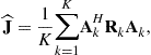
Receiver outputs are sampled as ![]() at frequency
at frequency ![]() , and sample covariance estimates of the visibility function (assuming zero mean signals) are obtained as
, and sample covariance estimates of the visibility function (assuming zero mean signals) are obtained as
 (20.34)
where N is the number of samples in the long term integration (LTI) window over which the imaging geometry and thus cross correlations may be assumed to be approximately stationary, and k is the LTI index. (We will later introduce a short term integration window length ![]() over which moving interference sources appear statistically stationary.)
over which moving interference sources appear statistically stationary.)
Since covariance estimates are only available at discrete time intervals (one per LTI index k), and the antennas have fixed Earth positions, only samples of ![]() are available with irregular spacing in the
are available with irregular spacing in the ![]() plane, so (20.32) must be solved with discreet approximations. However, noting that due to Earth rotation, the corresponding antenna position vector orientations
plane, so (20.32) must be solved with discreet approximations. However, noting that due to Earth rotation, the corresponding antenna position vector orientations ![]() depend on time through k, a new set of
depend on time through k, a new set of ![]() samples with different locations is available at each LTI. Index k is thus added to the notation to distinguish distinct baseline vectors
samples with different locations is available at each LTI. Index k is thus added to the notation to distinguish distinct baseline vectors ![]() for the same antenna pairs during different LTIs. So the (l, m)th element of
for the same antenna pairs during different LTIs. So the (l, m)th element of ![]() relates to the sampled visibility function as
relates to the sampled visibility function as
![]() (20.35)
(20.35)
where ![]() and where as in (20.26) and (20.31), due to inserted time delays
and where as in (20.26) and (20.31), due to inserted time delays ![]() we may take
we may take ![]() to be zero. For simplicity we will use a single index
to be zero. For simplicity we will use a single index ![]() to represent unique LTI-antenna index triples
to represent unique LTI-antenna index triples ![]() to specify vector samples in the
to specify vector samples in the ![]() plane, so
plane, so ![]() and
and ![]() . Thus elements of the sequence of matrices
. Thus elements of the sequence of matrices ![]() provide a non-uniformly sampled representation of the visibility function, or frequency domain image. Consistent with the treatment of
provide a non-uniformly sampled representation of the visibility function, or frequency domain image. Consistent with the treatment of ![]() in (20.32), diagonal elements in
in (20.32), diagonal elements in ![]() are set to zero.
are set to zero.
Figure 20.15a presents an example of a certain VLA geometry, and Figure 20.15b shows where the ![]() samples would lie, with each point representing a unique sample
samples would lie, with each point representing a unique sample ![]() . This plot includes 61 LTIs (i.e.,
. This plot includes 61 LTIs (i.e., ![]() ) over a 12 h VLA observation for the Cygnus A radio galaxy of Figure 20.12a. This sample pattern would change for sources with different positions on the celestial sphere (expressed by astronomers in right ascension and declination).
) over a 12 h VLA observation for the Cygnus A radio galaxy of Figure 20.12a. This sample pattern would change for sources with different positions on the celestial sphere (expressed by astronomers in right ascension and declination).
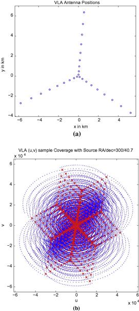
Figure 20.15 (a) An example VLA antenna element geometry with the repositionable 25 m dishes in a compact log spacing along the arms. Axis units are in kilometers. (b) Corresponding ![]() sample grid for a 12 h observation of Cygnus A. Each point represents a
sample grid for a 12 h observation of Cygnus A. Each point represents a ![]() sample corresponding to a unique baseline vector where a visibility estimate
sample corresponding to a unique baseline vector where a visibility estimate ![]() is available. Red crosses denote baselines from a single LTI midway through the observation, and blue points are additional samples available using Earth rotation, with a new
is available. Red crosses denote baselines from a single LTI midway through the observation, and blue points are additional samples available using Earth rotation, with a new ![]() computed every 12 min. Observation is at 1.61 GHz and axis units are in wavelengths. (For interpretation of the references to color in this figure legend, the reader is referred to the web version of this book.)
computed every 12 min. Observation is at 1.61 GHz and axis units are in wavelengths. (For interpretation of the references to color in this figure legend, the reader is referred to the web version of this book.)
With this frequency domain sampling and including noise effects (20.32) becomes
![]() (20.36)
(20.36)
![]() (20.37)
(20.37)
where ![]() is known as the “dirty image,” the sampling function
is known as the “dirty image,” the sampling function ![]() , and
, and ![]() represents sample estimation error in the covariance/visibility. Since the
represents sample estimation error in the covariance/visibility. Since the ![]() plane is sparsely sampled,
plane is sparsely sampled, ![]() introduces a bias in the inverse which must be removed by deconvolution as described below. This also means that (20.37) is not a true inverse Fourier transform due to the limited set of basis functions used. It is referred to as the “direct Fourier inverse” solution.
introduces a bias in the inverse which must be removed by deconvolution as described below. This also means that (20.37) is not a true inverse Fourier transform due to the limited set of basis functions used. It is referred to as the “direct Fourier inverse” solution.
There are two common approaches to solving (20.36) or (20.37) for ![]() given a set of LTI covariances
given a set of LTI covariances ![]() . The most straightforward though computationally intensive method is a brute force evaluation of (20.37) given knowledge of the
. The most straightforward though computationally intensive method is a brute force evaluation of (20.37) given knowledge of the ![]() sample locations (e.g., as in Figure 20.15). Alternately, the efficiencies of a 2-D inverse FFT can be exploited if these samples and corresponding visibilities
sample locations (e.g., as in Figure 20.15). Alternately, the efficiencies of a 2-D inverse FFT can be exploited if these samples and corresponding visibilities ![]() are re-sampled on a uniform rectilinear grid in the
are re-sampled on a uniform rectilinear grid in the ![]() plane. “Cell averaging” assigns the average of visibility samples contained in a local cell region to the new rectilinear grid point in the middle of the cell. Other re-gridding methods based on higher order 2-D interpolation have also been used successfully. When large fields of view are required, or array elements are not coplanar, then any of these approaches based on (20.31) will not work and a solution to the more complete expression of (20.30) must be found. Cornwell has developed the W-Projection method to address these conditions [27].
plane. “Cell averaging” assigns the average of visibility samples contained in a local cell region to the new rectilinear grid point in the middle of the cell. Other re-gridding methods based on higher order 2-D interpolation have also been used successfully. When large fields of view are required, or array elements are not coplanar, then any of these approaches based on (20.31) will not work and a solution to the more complete expression of (20.30) must be found. Cornwell has developed the W-Projection method to address these conditions [27].
An alternate “parametric matrix” representation of (20.31) and (20.37) has been developed. This is particularly convenient because it models the imaging system in a familiar array signal processing form that lends itself readily to analysis, adaptive array processing and interference canceling, and opens up additional options for solving the synthesis imaging and image restoration problems. Returning to the indexing notation of (20.34), note that since ![]() one may express
one may express ![]() as
as ![]() . Let
. Let ![]() be the desired image as scaled (i.e., vignetted) by the antenna beam pattern, and sample it on a regular 2-D grid of pixels
be the desired image as scaled (i.e., vignetted) by the antenna beam pattern, and sample it on a regular 2-D grid of pixels ![]() . The conventional visibility Eq. (20.31) then becomes
. The conventional visibility Eq. (20.31) then becomes
 (20.38)
 (20.39)
which in matrix form is
![]() (20.40)
(20.40)
![]() (20.41)
(20.41)
![]() (20.42)
(20.42)
and where ![]() is the diagonal image matrix representation of sampled
is the diagonal image matrix representation of sampled ![]() , M is the total number of array elements, and though noise is independent across antennas, the self noise terms have been included to allow for the
, M is the total number of array elements, and though noise is independent across antennas, the self noise terms have been included to allow for the ![]() case that contributes to the diagonal of full matrix
case that contributes to the diagonal of full matrix ![]() . The matrix discrete “direct Fourier inverse” relationship corresponding to (20.37) is
. The matrix discrete “direct Fourier inverse” relationship corresponding to (20.37) is
 (20.43)
where K is the number of available LTIs. Equations (20.40) and (20.43) are well suited to address synthesis imaging as an estimation problem, facilitating use of Maximum Likelihood, maximum a posteriori, constrained minimum variance, or robust beamforming techniques. Note that (20.43) is not a complete discrete inverse Fourier transform, indeed, often ![]() so a one-to-one inverse relationship between
so a one-to-one inverse relationship between ![]() and
and ![]() does not exist and
does not exist and ![]() is significantly blurred.
is significantly blurred.
By the Fourier convolution theorem, the effect of frequency sampling by ![]() in (20.36) is to convolve the desired image
in (20.36) is to convolve the desired image ![]() with the “dirty beam response”
with the “dirty beam response” ![]() . Neglecting the effect of individual antenna directivity pattern
. Neglecting the effect of individual antenna directivity pattern ![]() can be interpreted as the point spread function, or synthetic beam pattern of the imaging array for the given observation scenario. Significant reduction of this blurring effect can be achieved by an image restoration/deconvolution step. The dirty image of (20.36) may be expressed as
can be interpreted as the point spread function, or synthetic beam pattern of the imaging array for the given observation scenario. Significant reduction of this blurring effect can be achieved by an image restoration/deconvolution step. The dirty image of (20.36) may be expressed as
![]() (20.44)
(20.44)
where ![]() is due to sample estimation error in the visibilities. Since antenna locations in the rotating
is due to sample estimation error in the visibilities. Since antenna locations in the rotating ![]() plane are known precisely over the full observation,
plane are known precisely over the full observation, ![]() is known to high accuracy, and with well calibrated dish antennas so is
is known to high accuracy, and with well calibrated dish antennas so is ![]() . Thus (20.44) may be solved as
. Thus (20.44) may be solved as
![]() (20.45)
(20.45)
where “![]() ” denotes deconvolution with respect to the right argument. Due to the spatial lowpass nature of dirty beam
” denotes deconvolution with respect to the right argument. Due to the spatial lowpass nature of dirty beam ![]() this problem is ill conditioned and must be regularized by imposing some assumptions about the image. The most popular reconstruction methods impose a sparse source distribution model and use an iterative source subtraction approach related to the original CLEAN algorithm [32]. The sparse model is justifiable for point-source images of star fields, and works well even with more complex distributions of gas and nebular structures given that much of the field of view is expected to be dark. Several variants and extensions to CLEAN have been proposed, some applying source subtraction in the spatial
this problem is ill conditioned and must be regularized by imposing some assumptions about the image. The most popular reconstruction methods impose a sparse source distribution model and use an iterative source subtraction approach related to the original CLEAN algorithm [32]. The sparse model is justifiable for point-source images of star fields, and works well even with more complex distributions of gas and nebular structures given that much of the field of view is expected to be dark. Several variants and extensions to CLEAN have been proposed, some applying source subtraction in the spatial ![]() domain, and some in the frequency
domain, and some in the frequency ![]() domain. Typically these have performance tuning parameters which astronomers adjust for most pleasing results. Thus the effective regularization term or mathematical optimization expression is often not known precisely and the process is a bit ad hoc, but solutions with higher contrast and resolution, and with reduced noise and reconstruction artifacts are preferred. Maximum entropy reconstruction has also been used effectively.
domain. Typically these have performance tuning parameters which astronomers adjust for most pleasing results. Thus the effective regularization term or mathematical optimization expression is often not known precisely and the process is a bit ad hoc, but solutions with higher contrast and resolution, and with reduced noise and reconstruction artifacts are preferred. Maximum entropy reconstruction has also been used effectively.
3.20.3.2 Astronomical phased array feeds
A new application for array signal processing in radio astronomy is phased array feeds (PAFs) where the traditional single large horn antenna feed at the focus of large telescope dish is replaced with a closely spaced (order of 1/2 wavelength) 2-D planar array of small antennas located at the dish focal plane. The primary motivation for such a system, as shown in Figure 20.16 is to form multiple simultaneous beams steered to cover a grid pattern in a field of view that is many times larger than the single pixel horn fed dish. PAFs are ideal for wide-field and survey instruments where it is desired to cover large regions of the sky in the shortest possible time. They provide the ability to capture a small image over the field of view, with one pixel per simultaneously formed beam, using a single snapshot pointing of the dish. Such systems have been referred to as “radio cameras.” Additional advantages of PAFs include sensitivity optimization with respect to the noise environment, and spatial interference cancelation capabilities (see Figure 20.16 and Section 3.20.3.3) albeit at the expense of increased hardware and processing complexity.
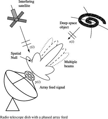
Figure 20.16 The primary advantage of FPA telescopes is increased field of view provided by multiple, simultaneously formed beams. Spatial cancelation of interfering signals is also possible, but very deep nulls are required.
In some ways PAF processing is simply conventional beamforming for an array of microwave receiving antennas, but there are several unique aspects of the application that provide some challenges. The following technical hurdles are why PAFs have not been previously adopted in radio astronomy, but these issues have largely been resolved and working platforms have now been demonstrated.
First, the PAF is not a bare aperture array but operates in conjunction with a very large reflector which for an on-axis far field point source focusses a tight Airy pattern spot of energy at the array that spans little more than a single array element. For off-axis sources the spot moves across the array and undergoes coma shaped pattern distortion. So, though noise and interference are seen on all elements, only a few antennas see much of the SOI. The combined dish and PAF can be viewed as a dense array of small but high gain, highly directive elements, but not all of these have equal SNR. Elements outside the focal spot must however be used in beamforming to control the illumination pattern on the dish and thus reduce spillover noise from observing warm ground beyond the edge of the dish. The focal properties of the dish also limit the achievable field of view, even with electronic steering, since deviation from the boresight axis beyond a few beamwidths leads to defocusing and loss of gain, no matter how large the PAF is.
Second, array calibration is critical to achieve maximum sensitivity (gain over noise power) and due to the huge sizes of these instruments, must be performed in situ using known deep space objects as calibration sources of opportunity. Calibrations must be performed periodically (order of weeks) to account for electronic and structural drift, and must estimate array response vectors in every direction that a beam is to be steered or a response constraint is to be placed.
Third, beamformer weight calculation is non-trivial. Astronomers want maximum sensitivity and stable beampatterns on the sky, but these competing requirements are challenging. The variable correlated noise field environment of a radio telescope calls for an adaptive approach, but it is difficult to obtain low error array calibrations at enough points to control beam sidelobe structure. Also, due to complexity of the antenna structures, it is impossible to design usable beamformer weights from even a very detailed electromagnetic system simulation.
Fourth, as discussed in Section 3.20.3.3, many of the conventional adaptive canceling beamforming methods are not very effective for astronomical PAFs. This is because observations are frequently done when both the SOI and interference power levels are well below the noise floor. New approaches are required to form deeper spatial nulls in scenarios where it is difficult to estimate interference parameters.
Fifth, replacing a single horn feed channel with 38, or 200 array elements, as have been proposed for PAFs, has major implications on the back end processing. Processed bandwidths of 300 MHz or more per antenna are needed, so a real-time DSP processor with capacity to serve as digital receiver, multiple beamformer, and array correlator for calibrationm constitutes a major infrastructure investment.
And finally, in a field where cryogenically cooled antennas and LNAs are the norm to reduce receiver noise, cooling a large array is daunting. Most current development projects have opted for room temperature arrays and trade off the then necessary longer integration times with faster survey speeds possible with multiple beams.
3.20.3.2.1 Signal model
After analog frequency down conversion, sampling, and complex baseband bandshifting, the array signal time sample vector of Figure 20.16 is modeled as
 (20.46)
where ![]() is the array response vector for signal of interest (SOI)
is the array response vector for signal of interest (SOI) ![]() is the time varying array response for the dth independent interfering source
is the time varying array response for the dth independent interfering source ![]() , and
, and ![]() is the noise vector. Source response
is the noise vector. Source response ![]() is assumed to be constant, even for observation times on the order of an hour because the dish mechanically tracks a point in the sky. Even fixed ground interference sources must be modeled as moving (thus
is assumed to be constant, even for observation times on the order of an hour because the dish mechanically tracks a point in the sky. Even fixed ground interference sources must be modeled as moving (thus ![]() depends on i) due to this tracking motion of the dish. Approaches to address man–made interference are discussed in Section 3.20.3.3. This model for
depends on i) due to this tracking motion of the dish. Approaches to address man–made interference are discussed in Section 3.20.3.3. This model for ![]() can also include natural deep space sources which are bright enough to overwhelm the SOI even when seen in the beam sidelobe pattern. Their apparent rotational motion about the SOI is due to Earth rotation. When the corresponding
can also include natural deep space sources which are bright enough to overwhelm the SOI even when seen in the beam sidelobe pattern. Their apparent rotational motion about the SOI is due to Earth rotation. When the corresponding ![]() is known accurately, these can be removed through a successive subtraction algorithm known as peeling. As with synthesis imaging, broadband processing for PAFs is accomplished by FFT based subband decomposition, often with thousands of frequency bins. So in the following we consider only a single frequency channel and adopt the standard narrowband array processing model.
is known accurately, these can be removed through a successive subtraction algorithm known as peeling. As with synthesis imaging, broadband processing for PAFs is accomplished by FFT based subband decomposition, often with thousands of frequency bins. So in the following we consider only a single frequency channel and adopt the standard narrowband array processing model.
Any array signal processing, including beamforming, must take into account the fact that, unlike synthesis imaging, the PAF noise vector ![]() is correlated across the array. Even with cryogenic cooling, first stage amplifier LNA noise is correlated due to electromagnetic mutual coupling at the elements. Another major component, spillover noise from warm ground black body radiation as seen by the feed array, is spatially correlated because it is not isotropic since it stops above the horizon and is blocked over a large solid angle by the dish.
is correlated across the array. Even with cryogenic cooling, first stage amplifier LNA noise is correlated due to electromagnetic mutual coupling at the elements. Another major component, spillover noise from warm ground black body radiation as seen by the feed array, is spatially correlated because it is not isotropic since it stops above the horizon and is blocked over a large solid angle by the dish.
In a practical PAF scenario the beams are steered in a rectangular or hexagonal grid pattern with crossover points at the −1 to −3 dB levels. The total number of beams, J, is limited by the maximum steering angle which is determined by the diameter of the array feed and the focal properties of the dish, by the acceptable limit for beamshape distortion, and by the available processing capacity for real-time simultaneous computation of multiple beams. As illustrated in Figure 20.17, the time series output for a beam steered in the jth direction is given by
![]() (20.47)
(20.47)
where ![]() is the vector of complex weights for beamformer
is the vector of complex weights for beamformer ![]() . Weights are designed based on array calibration data and the desired response pattern constraints and optimization as described in the following two sections. Separate beamformers with their own sets of J distinct weight vectors are computed for each frequency channel, though we consider only a single channel in this discussion.
. Weights are designed based on array calibration data and the desired response pattern constraints and optimization as described in the following two sections. Separate beamformers with their own sets of J distinct weight vectors are computed for each frequency channel, though we consider only a single channel in this discussion.

3.20.3.2.2 Calibration
Since multiple simultaneous beams are formed with a PAF as shown in Figure 20.16, a calibration for the signal array response vector ![]() must be performed for each direction,
must be performed for each direction, ![]() , corresponding to each formed beam’s boresight direction, and any additional directions where point constraints in the beam pattern response will be placed. Periodic re-calibration is necessary due to strict beam pattern stability requirements, to correct for differential electronic phase and gain drift, and to characterize changes in receiver noise temperatures. Calibration is based on sample array covariance estimates
, corresponding to each formed beam’s boresight direction, and any additional directions where point constraints in the beam pattern response will be placed. Periodic re-calibration is necessary due to strict beam pattern stability requirements, to correct for differential electronic phase and gain drift, and to characterize changes in receiver noise temperatures. Calibration is based on sample array covariance estimates ![]() as described in (20.34) while observing a dominant bright calibration point source in the sky. For example, in the northern hemisphere, Cassiopeia A and Cygnus A shown in Figure 20.12 are the brightest continuum (broadband) sources, and with a typical single dish telescope aperture they are unresolved and appear as point sources. Both have been used as calibrators.
as described in (20.34) while observing a dominant bright calibration point source in the sky. For example, in the northern hemisphere, Cassiopeia A and Cygnus A shown in Figure 20.12 are the brightest continuum (broadband) sources, and with a typical single dish telescope aperture they are unresolved and appear as point sources. Both have been used as calibrators.
3.20.3.2.3 Beamformer calculation
Since discovery of the weakest, most distant sources is a primary aim of radio astronomers, it is paramount to design a dish and feed combination to achieve high sensitivity, which has been derived for a phased array feed to be
![]() (20.48)
(20.48)
where ![]() (in
(in ![]() ) represents directivity in terms of the effective antenna aperture collecting area,
) represents directivity in terms of the effective antenna aperture collecting area, ![]() is system noise power at the beamformer output expressed as a black body temperature,
is system noise power at the beamformer output expressed as a black body temperature, ![]() is Boltzmann’s constant, B is system bandwidth,
is Boltzmann’s constant, B is system bandwidth, ![]() , (in Watts/m2) is the signal flux density in one polarization, and
, (in Watts/m2) is the signal flux density in one polarization, and ![]() and
and ![]() are the signal and noise components of
are the signal and noise components of ![]() respectively. Here we have assumed
respectively. Here we have assumed ![]() , i.e., that there are no interferers. For a reflector antenna with a traditional horn feed, maximizing sensitivity involves a hardware-only tradeoff between aperture efficiency, which determines the received signal power, and spillover efficiency, which determines the spillover noise contribution. With a PAF, sensitivity is determined by the beamforming weights as well as the array and receivers. Adjusting
, i.e., that there are no interferers. For a reflector antenna with a traditional horn feed, maximizing sensitivity involves a hardware-only tradeoff between aperture efficiency, which determines the received signal power, and spillover efficiency, which determines the spillover noise contribution. With a PAF, sensitivity is determined by the beamforming weights as well as the array and receivers. Adjusting ![]() controls both the PAF illumination pattern on the dish which affects
controls both the PAF illumination pattern on the dish which affects ![]() , and the response to the noise field, which affects
, and the response to the noise field, which affects ![]() . Noting that all other right hand side terms in (20.48) are constant, sensitivity can be maximized with the well known maximum signal to noise ratio (SNR) beamformer
. Noting that all other right hand side terms in (20.48) are constant, sensitivity can be maximized with the well known maximum signal to noise ratio (SNR) beamformer
![]() (20.49)
(20.49)
To date all hardware demonstrated PAF telescopes have used this maximum sensitivity beamformer. However, a hybrid beamformer design method for PAFs that parametrically trades off sensitivity maximization with constraining mainlobe shape and sidelobe levels has been proposed.
3.20.3.2.4 Radio camera results
In 2008, ASTRON and BYU/NRAO independently demonstrated the first radio camera images with a PAF fed dish. Figure 20.18 presents an example of the BYU work as a mosaic image of a complex source distribution in the Cygnus X region. As a comparison, the right image is from the Canadian Galactic Plane Survey image, but blurred by convolution with the equivalent beam pattern of the 20-Meter Telescope to match resolution scales. We expect that the image artifacts caused by discontinuities at mosaic tile boundaries could be eliminated with more sophisticated processing. The Cygnus X radio camera image contains approximately 3000 pixels. A more practical coarse grid spacing of about half the HPBW would require about 600 pixels. A single horn feed would require 600 pointings (one for each pixel) to form such an image, compared to 25 (one for each mosaic tile) for the radio camera. Thus for equal integration times per pixel, this radio camera provides an imaging speed up of 24 times.

Figure 20.18 (a) Cygnus X region at 1600 MHz. ![]() mosaic of images using the 19-element prototype PAF on the Green Bank 20-Meter Telescope. The circle indicates the half-power beamwidth. (b) Canadian Galactic Plane Survey image [38] convolved to the 20-m effective beamwidth. The center of the map is approximately
mosaic of images using the 19-element prototype PAF on the Green Bank 20-Meter Telescope. The circle indicates the half-power beamwidth. (b) Canadian Galactic Plane Survey image [38] convolved to the 20-m effective beamwidth. The center of the map is approximately ![]() (J2000) with north to the upper left. Credit: Karl Warnick in [33].
(J2000) with north to the upper left. Credit: Karl Warnick in [33].
3.20.3.3 Interference mitigation for radio astronomy
From a regulatory and spectrum management point of view, radio astronomy is a passive wireless service which must co-exist with many other licensed communications activities. Though international treaties have long been established to protect a few important frequency bands for astronomical use only (e.g., around 1420 MHz for emission lines of abundant deep space neutral Hydrogen) these precautions have become wholly inadequate. Astronomers’ current scientific goals require observing emissions across the radio spectrum from molecules of more exotic gas compounds, from broad spectrum sources such as pulsars, and from highly red shifted objects nearing the edge of the observable universe where Doppler effects dramatically reduce the frequencies. Thus there is virtually no frequency band devoid of interesting sources to study. Astronomers cannot rely solely on protected bands and must develop methods to mitigate ubiquitous man-made radio transmission interference.
The problem is further exacerbated because one of the fundamental aims of radio astronomy is to discover the weakest of sources which are often at signal levels many tens of decibels below the noise floor. Successful detection usually requires long integration times on the order of hours to average out noise induced sample estimation error variance, combined with on-source minus off-source subtraction to find subtile differences in power levels between a noise-only background and noise plus SOI. Thus even very weak interference levels that would hardly hinder wireless communications can completely obscure an astronomical source of interest.
There is a long laundry list of troublesome RFI sources for radio astronomy. Examples of man-made signals encountered at radio observatories for which mitigation strategies have been demonstrated include: satellite downlink transmissions, radar systems, air navigation aids, wireless communications, and digital television broadcasts. Even locating instruments in undeveloped areas with regulatory protection for radio quiet zones does not avoid many man-made sources such as satellite downlinks. Low frequency synthesis arrays such as LOFAR, PAPER, LWA, and the Murchison Widefield Array operate in the heavily used VHF bands (30–300 MHz) to detect highly redshifted emissions, and as such must contend with very powerful commercial TV and FM radio broadcasts, as well as two-way mobile communications services.
There are a variety of RFI mitigation methods used in radio astronomy. The major approaches include avoidance (simply wait until the interference stops or observe in a different frequency band), temporal excision (blank out only the small percentage of data samples corrupted by impulsive interference), waveform subtraction (estimate parameters for known structured interference and subtract a synthetic copy of this signal from the data), anti-coincidence (remove local interference by retaining only signals common to two distant observing stations), and spatial filtering (adaptive array processing to place spatial nulls on interference). Since this present article emphasizes array signal processing, we will address spatial filtering in the following discussion.
Figures 20.16 and 20.19 illustrate interference scenarios for a phased array feed and synthesis imaging array respectively. For PAFs the closely packed antennas in the feed enable for the first time adaptive spatial filtering on single dish telescopes. This would also be possible with PAFs on the multiple dishes of a large imaging array, but even with just typical single horn feeds (as in Figure 20.19) the covariance matrix used to compute imaging visibilities as in (20.34) and (20.40) can also be used for interference canceling. Some proposed algorithms use only the main imaging array antennas, while others achieve improved performance with additional smaller auxiliary antennas trained on the interferers as shown in the figure. The various algorithm approaches will be discussed below. Most spatial filtering work to-date has been at frequencies in L-band (1–2 GHz) and below because this includes important astronomical sources and because of the abundance of man-made interference in these bands.

Figure 20.19 An RFI scenario at a synthesis imaging array. Two independent interference sources are illustrated: a satellite downlink and a ground-based broadcast transmitter. The main imaging array consists of typical single feed dishes (i.e., PAF feeds are not used here). In addition to the main array, a subarray of smaller auxiliary antennas is shown which can be used with some algorithms discussed below to improve cancelation performance. If tracking information is available, these auxiliaries are steered to the offending sources to provide a high INR copy of the interference.
3.20.3.3.1 Challenges and solutions to radio astronomical spatial filtering
Many of the well-known adaptive beamforming algorithms appear at first glance to be promising candidates for interference mitigation in astronomical array processing, including maximum SNR, minimum variance distortionless response (MVDR or Capon), linearly constrained minimum variance (LCMV), generalized sidelobe canceler (GSC), Wiener filtering, and other algorithms. Robust canceling beamformers which are less sensitive to calibration error have also been considered for aperture arrays used as stations in large low frequency imaging arrays like LOFAR. However, due to several challenging characteristics of the radio astronomical RFI problem, most of these approaches are less successful here than they would be in typical radar, sonar, wireless communications, or signal intercept applications. These problems have made many astronomers reluctant to adopt the use of adaptive array processing methods for regular scientific observations. We note though that the intrinsic motivations to observe in RFI corrupted bands are becoming strong enough that rapid progress toward adoption is necessary and is anticipated by most practitioners. New algorithm adaptations are being introduced which are better suited for radio astronomical spatial filtering. We consider below some of the significant aspects of radio astronomy that complicate spatial filtering.
The typical astronomical SOI power level is 30 dB or more below the system noise over comparable bandwidth, even when cryogenically cooled LNAs are used with instruments located in radio quiet zones. Canceling nulls must therefore be deep enough to drive interference below the SOI level, i.e., below the on-source minus off-source detection limit, not just down to the system noise level. Most algorithms require a dominant interferer to form deep nulls because minimum variance methods (MVDR, LCMV, max SNR, Wiener Filtering, etc.) which balance noise variance with residual interference power cannot drive a weaker interferer far below the noise floor. The residual will remain well above the SOI level.
Another promising solution to limited null depth is a zero forcing beamformer like subspace projection (SP) where the null in the estimated vector subspace for interference is theoretically infinitely deep. A number of proposed radio astronomical RFI cancelers have adopted the SP approach and some experimental demonstration results have appeared. Figure 20.20 illustrates the first use of subspace projection RFI mitigation with a PAF as reported in [53]. Data were collected from a 19 element PAF mounted on the 20-Meter Telescope at the NRAO Green Bank, West Virginia observatory while observing the deep space Hydroxl Ion (OH) maser radiation source designated in star catalog as “W3OH.” An FM-modulated RFI source overlapping the W3OH spectral line at 1665 MHz was created artificially using a signal generator. The RFI was removed using the subspace projection algorithm. Snapshot radio camera images (see Section 3.20.3.2) of the source with and without RFI mitigation are shown in Figure 20.20. The source which was completely obscured by interference is now clearly visible.
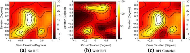
Figure 20.20 W3OH image with and without RFI. The color scale is equivalent antenna temperature (K).
Typically interference subspace estimation is poor in SP and all other cancelers without a dominant RFI signal so null depth suffers at lower INR levels. Short integration times, needed to avoid subspace smearing with moving interference, increase covariance sample estimation error which also limits null depth. To address these issues, an SP canceler using auxiliary antennas as in Figure 20.19 and a new parametric model-based SP approach for tracking low INR moving interferers have been proposed which significantly improves null depth [50].
Adaptive beamformers must distort the desired quiescent (interference free) beam pattern in order to place deep nulls on interferers. For astronomy, even modest beamshape distortions can be unacceptable. A small pointing shift in mainlobe peak response, or coma in the beam mainlobe can corrupt sensitive calibrated measurements of object brightness spatial distribution. Due to strict gain stability requirements it has been preferable to lose some observation time and frequency bands to interference rather than draw false scientific conclusions from corrupted on-sky beam patterns.
For PAF beamforming a potential solution is to use one of several classical constrained adaptive beamformers. Due to the inherent tendency for off-axis steered beams with a parabolic dish reflector to develop a mainlobe coma distortion, it would be necessary to employ several mainlobe point constraints to maintain a consistent symmetric beampattern. It has also been demonstrated that without multiple mainlobe constraints, RFI canceling nulls in the beampattern sidelobes can cause significant distortion in the mainlobe.
A more subtle undesirable effect for both PAF and synthesis imaging arrays is that variations in the effective sidelobe patterns due to moving RFI nulling can translate directly to an increase in the minimum detectable signal level for the radiometer. Weak astronomical sources can only be observed by integrating the received power for a long period to obtain separate low variance estimates of signal plus noise power (on source), and noise only (off source). Both signal and noise (including leakage from other deep space source through beam sidelobe patterns) must be stable to an extreme tolerance requirement over the full integration time. Even small variations in the sidelobe structure can significantly perturb background source and noise signal levels, causing intolerable time variation. This sidelobe pattern rumble due to adaptive cancelation increases the “confusion limit” to detection since unstable noise and background are not fully canceled in the on-source minus off-source subtraction. This occurs even if the beam pattern mainlobe is held stable using constrained or robust beamformer techniques.
3.20.4 Positioning and navigation
The Global Positioning System (GPS) is the most widely adopted positioning system in the world. It is a prominent example of what is known as Global Navigation Satellite Systems or GNSS, which represent any system that provides position information to users equipped with appropriate receivers at any time and anywhere around the globe based on signals transmitted from satellites. Currently there are two operating GNSS: GPS (developed by the USA) and Glonass (developed by the former USSR and now by Russia), while there are a number of systems under deployment, such as Galileo in Europe and Compass in China. Despite the differences in the satellite constellation, signal parameters, etc., all of these systems share the same operating principles and use similar types of signals. Therefore, while we will often refer to the case of GPS, all of what we discuss here is also applicable to the other systems as well.
The GPS constellation is formed by approximately 30 satellites orbiting at a distance of about 26,560 km from earth’s center. Each satellite transmits several Direct-Sequence Spread-Spectrum (DS-SS) signals, and the main task of a GPS receiver is to measure the distances to the satellites via the time delay of the signals. In applications requiring high-accuracy positions, the phase of the received signal is also used as a source of information about the propagation delay of the signal. Once the receiver has obtained these distances, it can compute its position by solving a geometrical problem. Apart from the satellites themselves, the core of a GNSS is the ground segment that consists of a set of ground stations monitoring the satellites and computing their positions.
Unlike communication receivers, where timing and phase synchronization are intermediary steps to recovering the transmitted information, for positioning receivers it is the synchronization that is the information. Significantly greater synchronization precision is required in a GNSS receiver than in a communications system. As discussed below, the positioning accuracy of GNSS is degraded by many effects. Multipath propagation and certain types of interference are very difficult to mitigate with single-antenna receivers. Spatial processing has proven to be the most effective approach to combat these sources of degradation, making it possible to obtain in some cases the same accuracy as in a multipath- and interference-free scenario. The next two sections describe the error sources in GNSS, with special emphasis on the multipath effects, and an appropriate signal model for spatial processing. They serve as a justification of why the use of antenna arrays in the context of GNSS has been receiving considerable attention since the mid-1990s. The rest of the sections discuss the advantages and limitations of different approaches for exploiting the spatial degrees of freedom or spatial diversity in satellite-based navigation systems.
3.20.4.1 Error sources and the benefits of antenna arrays in GNSS
The synchronization accuracy demanded by GPS receivers is very stringent, on the order of a few nanoseconds, and exceeds by far the levels usually required in communications receivers. The difficulties in achieving such ranging accuracy are due to the presence of different sources of error, which can be categorized in three groups: (i) the errors due to the ground segment and the satellites, (ii) propagation-induced errors, and (iii) local errors at the receiver. The first category includes the discrepancy between the estimates of the satellite positions and clocks, which are computed by the ground segment and broadcast by the satellites themselves, and the actual values. The second category corresponds to the changes in the propagation delay, phase and amplitude of the signals caused by the atmosphere. Finally, local errors refer to the effects of thermal noise, interference and multipath components.
The largest contributors to the total error budget are typically the ionospheric delay and local effects. The size of the errors in the first category is progressively decreasing as the ground segment and satellites are modernized. Moreover, one can also access alternative providers of more accurate satellite coordinates and clocks. Another option is to use differential methods, where the user receiver makes use of corrections computed by another receiver at a known position, or relative methods, where the position relative to that second receiver is computed. The use of differential or relative methods virtually eliminates the errors from the first category. These methods also help mitigate the propagation-induced errors. Alternatively, the ionospheric delay can be essentially canceled using measurements at two or more frequency bands. In short, the errors from the first two categories can typically be mitigated at the measurement or system levels, and hence the local errors remain as the limiting factor in the ultimate accuracy achievable with GNSS. This is the reason why it is of high interest to use signal processing techniques, and in particular antenna array-based methods, to combat multipath and interference effects in GNSS.
As in other systems, interference obviously affects the quality of time delay and phase estimates in GNSS. On the other hand, the study of multipath effects requires a different treatment to the one that is typically employed in wireless communications. While multipath components can be useful in communications systems as a source of diversity or to increase the total received signal power, they are always a source of error in navigation systems, and can lead to positioning inaccuracies reaching up to many tens of meters. For the case of a satellite-based transmission, multipath is produced by objects that are close to the receiver, as depicted in Figure 20.21. The only signal of interest in a navigation receiver is the line-of-sight (LOS) signal, since it conveys information about the transmitter-receiver distance through its time delay and phase information. While the multipath in a frequency-flat channel with zero delay-spread theoretically arrives at the same time as the LOS, the resulting fading can lead to signal drop-outs and poor localization performance. A second antenna (i.e., forming a small array) can be used to overcome this difficulty. More challenging are multipath signals that arrive with non-zero delay relative to the LOS, but still within 1–1.5 chip periods of the LOS (for civilian GPS, the chip period is 1 μs, corresponding to about 300 m). Such signals are commonly referred to as coherent multipath, and cause biases in the LOS signal time delay and carrier phase estimates. Signal replicas with delays greater than about 1.5 chip periods can essentially be eliminated via the despreading process.

Narrowband or pulsed interference can be canceled in single antenna receivers using excision filters or pulse blanking. Wideband non-pulsed interference cannot be combatted with time-domain processing, but it is in principle an easy target for array processing. Harmful interference usually stands out clearly above the noise, and this makes its identification and subsequent nulling with a spatial filter relatively easy. On the other hand, multipath mitigation is an extremely difficult task in single-antenna receivers and also a difficult problem when using antenna arrays. In the single-antenna case where time-domain methods must be used, the problem is ill-conditioned since one is attempting to estimate the parameters of signal replicas that are very similar to each other. If a reflection and the LOS signal differ by a very small delay (compared to the inverse of the signal bandwidth), they are almost identical and it is very difficult to accurately measure the exact LOS signal delay. On the other hand, the spatial selectivity offered by antenna arrays can be used to differentiate the LOS signal from multipath, since the multipath will arrive from directions different from the LOS (it is very unlikely to have reflectors close to the direct propagation path). The application of spatial processing for multipath mitigation is not without difficulties. The main problem is that the LOS signal and the coherent multipath are strongly correlated, which causes problems for many array processing techniques.
3.20.4.2 Signal model for positioning applications
The signal received by the antenna array can be written as
 (20.50)
In particular, in our problem the sources are not different signals, but delayed replicas of a single signal. Each replica is shifted by a different Doppler frequency ![]() , and its complex amplitude is
, and its complex amplitude is ![]() . The subindex 0 is reserved for the LOS signal, and this implies that
. The subindex 0 is reserved for the LOS signal, and this implies that ![]() . The term
. The term ![]() includes the thermal noise and any (possibly directional) interference. The key parameters of interest for positioning applications are
includes the thermal noise and any (possibly directional) interference. The key parameters of interest for positioning applications are ![]() and possibly the argument of
and possibly the argument of ![]() (i.e.,
(i.e., ![]() , which is the carrier phase of the LOS signal).
, which is the carrier phase of the LOS signal).
According to the discussion above, we assume that the delays of the replicas are in the range ![]() , where
, where ![]() is the chip duration. Each replica may represent a single reflection or a cluster of reflections with very similar delays. This leads to different possible parameterizations for the vectors
is the chip duration. Each replica may represent a single reflection or a cluster of reflections with very similar delays. This leads to different possible parameterizations for the vectors ![]() , as listed below:
, as listed below:
1. an unstructured spatial signature (i.e., each ![]() is an arbitrary complex vector). In this case, there is an inherent ambiguity between the definition of
is an arbitrary complex vector). In this case, there is an inherent ambiguity between the definition of ![]() and
and ![]() , which can be simply avoided by defining
, which can be simply avoided by defining ![]() as the overall spatial signature. One element of the spatial signature is identified as
as the overall spatial signature. One element of the spatial signature is identified as ![]() , and hence the carrier phase of the LOS signal is given by the argument of that element of the spatial signature.
, and hence the carrier phase of the LOS signal is given by the argument of that element of the spatial signature.
2. a steering vector (or also referred to as structured spatial signature), which is a function of the DOA.
3. a weighted sum of steering vectors: ![]() , where each term corresponds to the amplitude and the steering vector of one of the reflections of the cluster. In this case, the ambiguity between
, where each term corresponds to the amplitude and the steering vector of one of the reflections of the cluster. In this case, the ambiguity between ![]() and
and ![]() can be handled in the same way as in the first model.
can be handled in the same way as in the first model.
The signal ![]() may represent the GNSS signal itself or the signal after some processing. The most common case of processing in our context is the despreading operation, which consists in cross-correlating the received signal with a local replica of the pseudorandom or pseudonoise (PN) sequence. In this case, the variable t in the signals may be interpreted as the correlation lag. Unlike communications receivers, a single correlation lag is not sufficient. A single correlation lag may be appropriate for data detection but in a GNSS receiver, where the timing of the PN sequence has to be measured, several correlation lags are required. The correlation of the incoming signal with the local sequence is usually computed as a multiply-integrate-and-dump operation, which is carried out for each lag. However, the despread signal, depicted in Figure 20.22, can also be interpreted as a portion of the output of a matched filter. Figure 20.23 shows how the reception of multiple replicas affects the shape of the despread signal, and it is clear from there that identifying the components that form the signal is a very complicated task.
may represent the GNSS signal itself or the signal after some processing. The most common case of processing in our context is the despreading operation, which consists in cross-correlating the received signal with a local replica of the pseudorandom or pseudonoise (PN) sequence. In this case, the variable t in the signals may be interpreted as the correlation lag. Unlike communications receivers, a single correlation lag is not sufficient. A single correlation lag may be appropriate for data detection but in a GNSS receiver, where the timing of the PN sequence has to be measured, several correlation lags are required. The correlation of the incoming signal with the local sequence is usually computed as a multiply-integrate-and-dump operation, which is carried out for each lag. However, the despread signal, depicted in Figure 20.22, can also be interpreted as a portion of the output of a matched filter. Figure 20.23 shows how the reception of multiple replicas affects the shape of the despread signal, and it is clear from there that identifying the components that form the signal is a very complicated task.

Figure 20.22 Qualitative example of the signal at one antenna after the despreading (parameter T is the symbol period: 20 ms in GPS C/A, and ![]() is the chip duration:
is the chip duration: ![]() in GPS C/A.)
in GPS C/A.)

Figure 20.23 Qualitative example of the despreaded signal composed of the LOS component and two reflections. These reflections are considered as coherent multipath because their contributions overlap with that of the LOS component.
The choice of whether to base the computation of beamformers or other estimation methods on the pre-despreading (pre-correlation) or post-despreading (post-correlation) signal has a crucial impact on the performance and limitations of the array processing algorithms. GNSS signals typically have a Carrier-Power-to-Noise-Spectral-Density ![]() of about 45 dB Hz. The chip rate and hence the bandwidth is greater than 1 MHz, so this results in an SNR on the order of −15 dB or less. This means that the GNSS signals and also their reflections are buried in the background noise. If one computes the spatial correlation matrix
of about 45 dB Hz. The chip rate and hence the bandwidth is greater than 1 MHz, so this results in an SNR on the order of −15 dB or less. This means that the GNSS signals and also their reflections are buried in the background noise. If one computes the spatial correlation matrix ![]() in a pre-correlation scheme, only the noise and interference have a noticeable contribution to the matrix, so in practical terms the “total” correlation matrix
in a pre-correlation scheme, only the noise and interference have a noticeable contribution to the matrix, so in practical terms the “total” correlation matrix ![]() really only represents the noise-plus-interference correlation matrix.
really only represents the noise-plus-interference correlation matrix.
The situation is completely different in the post-correlation scheme. The SNR of the correlation maximum is equal to ![]() times the duration of the local reference. The duration of PN sequences in GNSS is several milliseconds, so the SNR of the maximum is typically on the order of several tens of dBs. The average SNR of the signal depends on the length of the portion of the correlation around the maximum that is taken as the observation window. This length is normally not too large, usually only a few chips, so the average SNR stays at the level of tens of dBs. In this case, the post-correlation matrix
times the duration of the local reference. The duration of PN sequences in GNSS is several milliseconds, so the SNR of the maximum is typically on the order of several tens of dBs. The average SNR of the signal depends on the length of the portion of the correlation around the maximum that is taken as the observation window. This length is normally not too large, usually only a few chips, so the average SNR stays at the level of tens of dBs. In this case, the post-correlation matrix ![]() includes noticeable contributions from the LOS and reflected signals besides the noise and interference. To conclude, in order to make multipath visible in the spatial correlation matrix, one has to work with the post-despreading correlation matrix. If one wants to hide multipath from the spatial correlation matrix, the pre-despreading correlation matrix has to be used.
includes noticeable contributions from the LOS and reflected signals besides the noise and interference. To conclude, in order to make multipath visible in the spatial correlation matrix, one has to work with the post-despreading correlation matrix. If one wants to hide multipath from the spatial correlation matrix, the pre-despreading correlation matrix has to be used.
The location of the beamformer (if any) with respect to the despreader has an impact on computational complexity, but it does not have an effect on performance since only its position within a set of linear operations is changed. Note that we are referring here to the placement of the beamformer in the receive chain, and not to the input data used for its computation, which is a totally different aspect as explained above. Some examples of the placement of the beamformer as well as the input data used for its computation are shown in Figures 20.24 and 20.25. Note that all combinations are in principle possible, although some cases, such as pre-despreading beamforming with weights computed using the post-despread signals, do not have a clear justification. As an example of a typical approach, the beamforming vector is computed using the pre-despread correlation matrix as ![]() , and applied to the despread signal to obtain
, and applied to the despread signal to obtain ![]() . In the first formula, the symbol
. In the first formula, the symbol ![]() refers to signals before despreading, whereas in the second formula it refers to the despread signals.
refers to signals before despreading, whereas in the second formula it refers to the despread signals.

Figure 20.24 Example of a GNSS receiver using an antenna array where the beamformer is applied before despreading and it is computed using the pre-despread signals. The output of the beamformer is processed by a conventional GNSS receiver channel, as if it was the signal coming from a single antenna. Either option is possible: the beamformer can be the same for all satellites, or different beamformers for different satellites can be used. The complexity bottleneck is due to the fact that the beamformer weights are applied to high-rate samples coming from the RF front-end.

Figure 20.25 Example of a GNSS receiver using an antenna array where the beamformer is applied after despreading. The beamformer vector is calculated using the pre-despreading or the post-despreading spatial correlation matrix. An optional spatial preprocessing block is included, which can be used to cancel some spatial sectors. The number of outputs of the preprocessing block, ![]() , is equal to or smaller than the number of antennas, M. In this configuration, the application of the beamformer weights do not entail a significant computational load because the correlation channels generate samples at a very low rate. Hence the fact that a different beamformer is applied for each satellite is not a problem. Here the computational bottleneck comes from the need to use a correlation channel at each antenna or at each output of the preprocessing block.
, is equal to or smaller than the number of antennas, M. In this configuration, the application of the beamformer weights do not entail a significant computational load because the correlation channels generate samples at a very low rate. Hence the fact that a different beamformer is applied for each satellite is not a problem. Here the computational bottleneck comes from the need to use a correlation channel at each antenna or at each output of the preprocessing block.
3.20.4.3 Beamforming
The objective is to synthesize an array pattern that attenuates the reflections and interference. In the context of GNSS, antenna-array beamformers are customarily referred to as CRPAs (Controlled Reception Pattern Antennas). Adaptive (or data-dependent) beamforming is appropriate for situations where little a priori information about the scenario is available, or when the scenario is likely to change with time. This is the typical situation for user receivers. On the other hand, deterministic (or data-independent) beamforming is more suitable for static and relatively controlled scenarios. This is typically the case for ground reference stations. These reference stations refer to both the receivers that form part of the ground segment of the GNSS (i.e., those receivers providing the measurements used to compute the position of the satellites) and the user receivers that are static and typically used as references in differential or relative positioning.
3.20.4.3.1 Adaptive beamforming
As outlined below, several different types of adaptive beamforming algorithms have been proposed for GNSS. Some of these are adaptations of standard algorithms, others have been designed specifically for conditions specific to positioning applications.
Algorithms employing a spatial reference: These approaches are based on knowledge of the steering vector of the LOS signal, ![]() . Assuming this a priori information is reasonable in some GNSS applications since the satellite position can be known thanks to the navigation message (transmitted by the satellite itself) or to assistance from ground stations, and a rough estimate of the receiver position may be available from previous position fixes or from the application of a basic positioning algorithm (e.g., using only one antenna and not exploiting the antenna array). Moreover, the accuracy of the satellite and receiver positions is not important in determining the DOA of the signal; errors of several hundreds of meters can be tolerated without affecting the satellite DOA estimate, given that the satellite-receiver distance is more than 20,000 km. However, the assumption of a known
. Assuming this a priori information is reasonable in some GNSS applications since the satellite position can be known thanks to the navigation message (transmitted by the satellite itself) or to assistance from ground stations, and a rough estimate of the receiver position may be available from previous position fixes or from the application of a basic positioning algorithm (e.g., using only one antenna and not exploiting the antenna array). Moreover, the accuracy of the satellite and receiver positions is not important in determining the DOA of the signal; errors of several hundreds of meters can be tolerated without affecting the satellite DOA estimate, given that the satellite-receiver distance is more than 20,000 km. However, the assumption of a known ![]() relies on the availability of array calibration and especially on the knowledge of the receiver orientation (also known as attitude in the GNSS literature). Errors or uncertainty in the array response correspond to the standard calibration problem found in many applications of antenna arrays, and robust methods developed for generic applications are also applicable here. On the other hand, the need to know the receiver orientation is a feature more specific to GNSS receivers. Assuming that
relies on the availability of array calibration and especially on the knowledge of the receiver orientation (also known as attitude in the GNSS literature). Errors or uncertainty in the array response correspond to the standard calibration problem found in many applications of antenna arrays, and robust methods developed for generic applications are also applicable here. On the other hand, the need to know the receiver orientation is a feature more specific to GNSS receivers. Assuming that ![]() is known, the use of the MVDR beamformer (and variants) is possible, and it is most appropriate to apply them in a pre-despreading scheme. If these beamformers are computed with the post-despreading correlation matrix and multipath components are present, they will suffer from the cancellation of the desired signal.
is known, the use of the MVDR beamformer (and variants) is possible, and it is most appropriate to apply them in a pre-despreading scheme. If these beamformers are computed with the post-despreading correlation matrix and multipath components are present, they will suffer from the cancellation of the desired signal.
Algorithms employing a temporal reference: These methods are based on knowledge of the GNSS signal waveform. Knowledge of the waveform can be exploited to design a beamformer that minimizes the difference between its output and the reference signal (e.g., as in a Wiener filter). In practice, the situation is not that straightforward because even though the shape of the signal is known, the delay and frequency shift are not, so the beamformer weights and the signal parameters have to be computed jointly or iteratively. The expression for the beamformer is
![]() (20.51)
(20.51)
where ![]() is the cross-correlation between the array output and a local replica of the LOS signal generated using estimates of its delay and frequency shift,
is the cross-correlation between the array output and a local replica of the LOS signal generated using estimates of its delay and frequency shift, ![]() and
and ![]() , respectively. In this case, it only makes sense to work with correlations computed after the despreading, otherwise the contribution of the GNSS signals is hardly present in the correlations. This beamformer is able to cancel interference, but its performance in the presence of multipath is not satisfactory, although not as bad as with spatial-reference beamformers. The temporal reference beamformer combines the multipath and the LOS signal in a constructive manner, so as to increase the SNR. This is useful behavior in communications but not in navigation systems, since the increase in SNR comes at the price of a bias in the estimation of the delay and phase due to the presence of strong multipath at the beamformer output.
, respectively. In this case, it only makes sense to work with correlations computed after the despreading, otherwise the contribution of the GNSS signals is hardly present in the correlations. This beamformer is able to cancel interference, but its performance in the presence of multipath is not satisfactory, although not as bad as with spatial-reference beamformers. The temporal reference beamformer combines the multipath and the LOS signal in a constructive manner, so as to increase the SNR. This is useful behavior in communications but not in navigation systems, since the increase in SNR comes at the price of a bias in the estimation of the delay and phase due to the presence of strong multipath at the beamformer output.
Hybrid beamformers: The opposite behavior of the spatial-reference and temporal-reference beamformers suggests that their combination may have good properties. Both of them provide the LOS signal at the output, but the former changes the phase of the multipath so that it is roughly in counter-phase with the LOS signal, whereas the later modifies the multipath phase to align it with that of the LOS signal. Therefore, if the output of both beamformers is added together, the multipath will tend to cancel. This observation has led to the proposal of a hybrid beamformer that can be expressed as
![]() (20.52)
(20.52)
where ![]() is a spatial-reference beamformer, and
is a spatial-reference beamformer, and ![]() and
and ![]() are two scalars weighting the contribution of each beamformer. When
are two scalars weighting the contribution of each beamformer. When ![]() is chosen as the MVDR beamformer, it can be shown that the optimal weights are
is chosen as the MVDR beamformer, it can be shown that the optimal weights are
![]() (20.53)
(20.53)
Since the optimal weights depend on the unknown parameters to be estimated, a practical way to proceed is to use an iterative algorithm where the calculation of the beamformer according to (20.52) is done using the previous estimates of ![]() , and next these estimates are updated using the output of the just computed beamformer.
, and next these estimates are updated using the output of the just computed beamformer.
Blind algorithms: This class of methods refers to techniques that do not exploit a priori knowledge of the exact signal or the steering vector, and hence are more robust to errors in these assumptions. Examples of such methods include those based on the constant modulus (CM) assumption, cyclostationarity and the power inversion approach. The civil GPS signal in current use, referred to as the C/A signal, has constant modulus because it is formed by almost rectangular chips. Most other GNSS signals also satisfy the CM property. However, this property cannot be exploited before despreading since the array cannot provide enough SNR gain to bring the signal above the noise. Therefore, the CM beamformer has to be applied after despreading, but in order to do so the despread samples corresponding to the LOS signal have to be CM. This happens when only one sample per integration period is used. However, the presence of multipath does not alter the constant-modulus property of the signal, so the CM beamformer is not useful in combating multipath.
GNSS signals are obviously cyclostationary since the repeated use of the PN spreading sequence introduces periodicity into the statistics of the signal. The fact that several repetitions of the PN code are present during a bit time (a property sometimes referred to as self-coherence) can also be exploited, as depicted in Figure 20.26. Interference will not have in general this structure, so it is possible to design the beamformer by imposing that its output should be as similar as possible to a version of itself delayed by a time equal to the PN code duration. Because of the same reasons as in the case of the CM beamformer, this technique should be applied to the despread signals and it will only be effective against interference and not multipath.

Figure 20.26 Structure of the GPS signal that allows to implement self-coherence restoration beamforming methods.
A very simple but rather effective approach is the power inversion beamformer. The weights are obtained as the beamformer vector that minimizes the total output power subject to a simple constraint to avoid the null solution. The constraint is chosen without using any information about the signal, typically forcing a given beamformer coefficient to be equal to one. This method has to be applied to the signals before despreading and, since the response is independent of the GNSS signals, it may happen that some nulls of the reception pattern are near to the DOAs of some of the GNSS signals. However, this situation can often be accepted since it is assumed that many GNSS satellites will be visible (around 10 satellites), and if a few of them are lost due to the coincidence of the pattern nulls with their DOAs, there will still be a sufficient number of satellite signals available (i.e., four or more) to compute the position. In this method, all satellites are received through the same beamformer, so it offers the possibility of being deployed as an add-onto existing single-antenna receivers. This is an important advantage of this method; more sophisticated beamformers that require information provided the receiver (e.g., the DOA or the delay of the LOS signal) or that generate one beam per satellite cannot be coupled with existing single-antenna receivers and require the development of a completely new receiver. The number of antennas used with power inversion should be large enough to cancel the existing interference sources, but not much larger in order not to increase the number of nulls in the pattern and thus the probability that a GNSS signal is canceled. The power inversion approach is popular in military systems where jamming from highly maneuverable sources (fighter jets) is a pivotal concern. The fast maneuvers of these vehicles makes the use of spatial-reference beamformers virtually impossible, and therefore a simple and robust method like power inversion, that does not need any reference or calibration procedure, is an excellent option.
3.20.4.3.2 Deterministic beamforming
Although it is recognized that data-dependent beamformers are more powerful in general than deterministic versions, there are some situations where the latter may be advantageous. Deterministic beamformers are clearly more robust against calibration errors and other uncertainties in the signal parameters. Moreover, if the desired and non-desired signals are known to be confined to distinct spatial regions, the deterministic design may offer an adequate solution since the problem reduces to designing a spatial filter with given pass and stop bands. This a priori spatial separability occurs in several circumstances in GNSS, particularly in GNSS ground stations. In this case, the interference is normally ground-based, and the multipath normally arises from ground-based scatterers, so both interference and multipath impinge on the receiver from relatively low elevation angles. This is contrasted with the satellite signals, which originate from the entire upper hemisphere. Thus, as illustrated in Figure 20.27, a fixed beamformer can be designed to minimize reception of signals from these low elevations. The complicating factor here is that an upwards-facing array typically cannot provide a sharp stop-band to pass-band transition for directions near end-fire. Another advantage of deterministic beamformers is that they allow an easier control of the trade-off between array gain (understood here as the increase of the ratio between the desired signal power and the white noise power) and interference cancellation. In adaptive beamformers, these two characteristics are tightly coupled. For instance, with MVDR, the presence of a strong interference gives rise to a deep null in the pattern, and this null necessarily increases the beampattern in other directions, thus degrading the array gain.