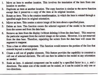
Chapter 6
Computer Graphics Software and Data Base
6.1 Introduction
The CAD hardware discussed in Chapter 5 would be useless without the software to support it. This chapter discusses some of the issues and methods related to the software and accompanying data base for interactive computer graphics and computer-aided design. A more complete coverage of this topic is available in several of the references listed at the end of the chapter. References [4] and [8] are comprehensive in their coverage of both hardware and software. References [2] and [10] are concerned more with the mathematics required in computer graphics.
The graphics software is the collection of programs written to make it convenient for a user to operate the computer graphics system. It includes programs to generate images on the CRT screen, to manipulate the images, and to accomplish various types of interaction between the user and the system. In addition to the graphics software, there may be additional programs for implementing certain specialized functions related to CAD/CAM. These include design analysis programs (e.g., finite-element analysis and kinematic simulation) and manufacturing planning programs (e.g., automated process planning and numerical control part programming). This chapter deals mainly with the graphics software.
The graphics software for a particular computer graphics system is very much a function of the type of hardware used in the system. The software must be written specifically for the type of CRT and the types of input devices used in the system. The details of the software for a stroke-writing CRT would be different than for a raster scan CRT. The differences between a storage tube and a refresh tube would also influence the graphics software. Although these differences in software may be invisible to the user to some extent, they are important considerations in the design of an interactive computer graphics system.
Newman and Sproull [8] list six “ground rules” that should be considered in designing graphics software:
1. Simplicity. The graphics software should be easy to use.
2. Consistency. The package should operate in a consistent and predictable way to the user.
3. Completeness. There should be no inconvenient omissions in the set of graphics functions.
4. Robustness. The graphics system should be tolerant of minor instances of misuse by the operator.
5. Performance. Within limitations imposed by the system hardware, the performance should be exploited as much as possible by software. Graphics programs should be efficient and speed of response should be fast and consistent.
6. Economy. Graphics programs should not be so large or expensive as to make their use prohibitive.
6.2 The Software Configuration of a Graphics System
In the operation of the graphics system by the user, a variety of activities take place, which can be divided into three categories:
1. Interact with the graphics terminal to create and alter images on the screen.
2. Construct a model of something physical out of the images on the screen. The models are sometimes called application models.
3. Enter the model into computer memory and/or secondary storage.
In working with the graphics system the user performs these various activities in combination rather than sequentially. The user constructs a physical model and inputs it to memory by interactively describing images to the system. This is done without any thought about whether the activity falls into category 1, 2, or 3.
The reason for separating these activities in this fashion is that they correspond to the general configuration of the software package used with the interactive computer graphics (ICG) system. The graphics software can be divided into three modules according to a conceptual model suggested by Foley and Van Dam [4]:
1. The graphics package (Foley and Van Dam called this the graphics system)
2. The application program
3. The application data base
This software configuration is illustrated in Figure 6.1. The central module is the application program. It controls the storage of data into and retrieves data out of the application data base. The application program is driven by the user through the graphics package.
The application program is implemented by the user to construct the model of a physical entity whose image is to be viewed on the graphics screen. Application programs are written for particular problem areas. Problem areas in engineering design would include architecture, construction, mechanical components, electronics, chemical engineering, and aerospace engineering. Problem areas other than design would include flight simulators, graphical display of data, mathematical analysis, and even artwork. In each case, the application software is developed to deal with images and conventions which are appropriate for that field.
The graphics package is the software support between the user and the graphics terminal. It manages the graphical interaction between the user and the system. It also serves as the interface between the user and the application software. The graphics package consists of input subroutines and output subroutines. The input routines accept input commands and data from the user and forward them to the application program. The output subroutines control the display terminal (or other output device) and converts the application models into two-dimensional or three-dimensional graphical pictures.
The third module in the ICG software is the data base. The data base contains mathematical, numerical, and logical definitions of the application models,
Figure 6.1 Model of graphics software configuration.
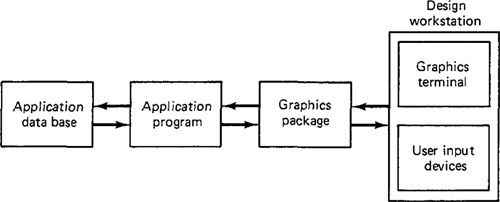
such as electronic circuits, mechanical components, automobile bodies, and so forth. It also includes alphanumeric information associated with the models, such as bills of materials, mass properties, and other data. The contents of the data base can be readily displayed on the CRT or plotted out in hard-copy form. Section 6.6 presents a discussion of the data base for computer graphics.
6.3 Functions of a Graphics Package
To fulfill its role in the software configuration, the graphics package must perform a variety of different functions. These functions can be grouped into function sets. Each set accomplishes a certain kind of interaction between the user and the system. Some of the common function sets are:
Generation of graphic elements
Transformations
Display control and windowing functions
Segmenting functions
User input functions
We examine some of these functions in more detail in subsequent sections of this chapter. What we present in the sections below is a brief description of each.
Generation of graphic elements
A graphic element in computer graphics is a basic image entity such as a dot (or point), line segment, circle, and so forth. The collection of elements in the system could also include alphanumeric characters and special symbols. There is often a special hardware component in the graphics system associated with the display of many of the elements. This speeds up the process of generating the element. The user can construct the application model out of a collection of elements available on the system.
The term “primitive” is often used in reference to graphic elements. We shall reserve the use of this term to three-dimensional graphics construction. Accordingly, a primitive is a three-dimensional graphic element such as a sphere, cube, or cylinder. In three-dimensional wire-frame models and solid modeling, primitives are used as building blocks to construct the three-dimensional model of the particular object of interest to the user.
Transformations
Transformations are used to change the image on the display screen and to reposition the item in the data base. Transformations are applied to the graphic elements in order to aid the user in constructing an application model. These transformations include enlargement and reduction of the image by a process called scaling, repositioning the image or translation, and rotation. We discuss two- and three-dimensional transformations in Section 6.5.
Display control and windowing functions
This function set provides the user with the ability to view the image from the desired angle and at the desired magnification. In effect, it makes use of various transformations to display the application model the way the user wants it shown. This is sometimes referred to as windowing because the graphics screen is like a window being used to observe the graphics model. The notion is that the window can be placed wherever desired in order to look at the object being modeled.
Another aspect of display control is hidden-line removal. In most graphics systems, the image is made up of lines used to represent a particular object. Hidden-line removal is the procedure by which the image is divided into its visible and invisible (or hidden) lines. In some systems, the user must identify which lines (or portions of lines) are invisible so that they can be removed from the image to make it more understandable. In other systems, the graphics package is sufficiently sophisticated to remove the hidden lines from the picture automatically.
Segmenting functions
Segmenting functions provide users with the capability to selectively replace, delete, or otherwise modify portions of the image. The term “segment” refers to a particular portion of the image which has been identified for purposes of modifying it. The segment may define a single element or logical grouping of elements that can be modified as a unit.
Storage-type CRT tubes are unsuited to segmenting functions. To delete or modify a portion of the image on a storage tube requires erasing the entire picture and redrawing it with the changes incorporated. Raster scan refresh tubes are ideally suited to segmenting functions because the screen is automatically redrawn 30 or more times per second anyway. The image is regenerated each cycle from a display file, a file used for storage that is part of the hardware in the raster scan CRT. The segment can readily be defined as a portion of that display file by giving it a name. The contents of that portion of the file would then be deleted or altered to execute the particular segmenting function.
User input functions
User input functions constitute a critical set of functions in the graphics package because they permit the operator to enter commands or data to the system. The entry is accomplished by means of operator input devices, and from Chapter 5 we note that there are a large variety of these input devices. The user input functions must, of course, be written specifically for the particular compliment of input devices used on the system. The extent to which the user input functions are well designed has a significant effect on how “friendly” the system is to the user, that is, how easy it is to work on the system.
The input functions should be written to maximize the benefits of the interactive feature of ICG. The software design compromise is to find the optimum balance between providing enough functions to conveniently cover all data entry situations without inundating the user with so many commands that they cannot be remembered. One of the goals that are sought after by software designers in computer graphics is to simplify the user interface enough that a designer with little or no programming experience can function effectively on the system.
6.4 Constructing the Geometry
The use of graphics elements
The graphics system accomplishes the definition of the model by constructing it out of graphic elements. These elements are called by the user during the construction process and added, one by one, to create the model. There are several aspects about this construction process which should be discussed.
First, as each new element is being called but before it is added to the model, the user can specify its size, its position, and its orientation. These specifications are necessary to form the model to the proper shape and scale. For this purpose, the various transformations mentioned previously are utilized.
A second aspect of the geometric construction process is that graphics elements can be subtracted as well as added. Another way of saying this is that the model can be formed out of negative elements as well as positive elements. Figure 6.2 illustrates this construction feature for a two-dimensional object, C. The object is drawn by subtracting circle B from rectangle A.
A third feature available during model building is the capability to group several elements together into units which are sometimes called cells. A cell, in this context, refers to a combination of elements which can be called to use any-
Figure 6.2 Example of two-dimensional model construction by subtraction of circle B from rectangle A.
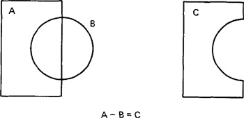
where in the model. For example, if a bolt is to be used several places in the construction of a mechanical assembly model, the bolt can be formed as a cell and added anywhere to the model. The use of graphic cells is a convenient and powerful feature in geometric model construction.
Defining the graphic elements
The user has a variety of different ways to call a particular graphic element and position it on the geometric model. Table 6.1 lists several ways of defining points, lines, arcs, and other components of geometry through interaction with the ICG system. These components are maintained in the data base in mathematical form and referenced to a three-dimensional coordinate system. For example, a point would be defined simply by its x, y, and z coordinates. A polygon would be defined as an ordered set of points representing the corners of the polygon. A circle would be defined by its center and radius. Mathematically, a circle can be defined in the x-y plane by the equation
(x - m)2 + (y - n2 = r2 (6.1)
This specifies that the radius of the circle is r and the xand y of the center are m and n. In each case, the mathematical definition can be converted into its corresponding edges and surfaces for filing in the data base and display on the CRT screen.
Editing the geometry
A computer-aided design system provides editing capabilities to make corrections and adjustments in the geometric model. When developing the model, the user must be able to delete, move, copy, and rotate components of the model. We have previously discussed some of these adjustments in our discussion of the functions of a graphics package in Section 6.3. The editing procedure involves selecting the desired portion of the model (usually by means of one of the segmenting functions), and executing the appropriate command (often involving one of the transformation functions).
The method of selecting the segment of the model to be modified varies from system to system. With cursor control, a common method is for a rectangle to be formed on the CRT screen around the model segment. The rectangle is defined by entering the upper left and lower right corners of the rectangle. Another method involving a light pen is to place the pen over the component to be selected. With the electronic pen and tablet, the method might be to stroke a line across the portion of the model which is to be altered.
The computer must somehow indicate to the user which portion of the model has been selected. The reason for this is verification that the portion selected by the computer is what the user intended. Various techniques are used by different ICG
Table 6.1 Methods of Defining Elements in Interactive Computer Graphics
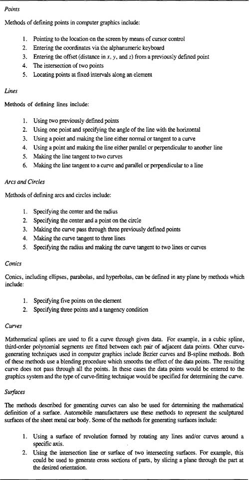
systems to identify the segment. These include: placing a mark on the segment, making the segment brighter than the rest of the image, and making the segment blink.
A selection of common editing capabilities available in commercial CAD systems is presented in Table 6.2.
Table 6.2 Some Common Editing Features Available on a CAD System
6.5 Transformations
Many of the editing features involve transformations of the graphics elements or cells composed of elements or even the entire model. In this section we discuss the mathematics of these transformations. Two-dimensional transformations are considered first to illustrate concepts. Then we deal with three dimensions.
Two-dimensional transformations
To locate a point in a two-axis cartesian system, the x and y coordinates are specified. These coordinates can be treated together as a 1 x 2 matrix: (x,y). For example, the matrix (2, 5) would be interpreted to be a point which is 2 units from the origin in the x-direction and 5 units from the origin in the y-direction.
This method of representation can be conveniently extended to define a line as a 2 X 2 matrix by giving the x and y coordinates of the two end points of the line. The notation would be
![]()
Using the rules of matrix algebra, a point or line (or other geometric element represented in matrix notation) can be operated on by a transformation matrix to yield a new element.
There are several common transformations used in computer graphics. We will discuss three transformations: translation, scaling, and rotation.
TRANSLATION. Translation involves moving the element from one location to another. In the case of a point, the operation would be
x’ = x + m, y' = y + n (6.3)
where x',y' = coordinates of the translated point
x,y = coordinates of the original point
m,n = movements in the x and y directions, respectively
In matrix notation this can be represented as
(x',y') = (x,y) + T (6.4)
where
T = (m,n), the translation matrix (6.5)
Any geometric element can be translated in space by applying Eq. (6.4) to each point that defines the element. For a line, the transformation matrix would be applied to its two end points.
SCALING. Scaling of an element is used to enlarge it or reduce its size. The scaling need not necessarily be done equally in the x and y directions. For example, a circle could be transformed into an ellipse by using unequal x and y scaling factors.
The points of an element can be scaled by the scaling matrix as follows:
(x',y') = (x,y)S (6.6)
where
![]()
This would produce an alteration in the size of the element by the factor m in the x-direction and by the n factor in the y direction. It also has the effect of repositioning the element with respect to the cartesian system origin. If the scaling factors are less than 1, the size of the element is reduced and it is moved closer to the origin. If the scaling factors are larger than 1, the element is enlarged and removed farther from the origin.
ROTATION. In this transformation, the points of an object are rotated about the origin by an angle 0. For a positive angle, this rotation is in the counterclockwise direction. This accomplishes rotation of the object by the same angle, but it also moves the object. In matrix notation, the procedure would be as follows:
(x',y') = (x,y)R (6.8)
![]()
Example 6.1
As an illustration of these transformations in two dimensions, consider the line defined by
![]()
Let us suppose that it is desired to translate the line in space by 2 units in the x direction and 3 units in the y direction. This would involve adding 2 to the current x value and 3 to the current y value of the end points defining the line. That is,
Figure 6.3. Results of translation in Example 6.1.

![]()
The new line would have end points at (3, 4) and (4, 7). The effect of the transformation is illustrated in Figure 6.3.
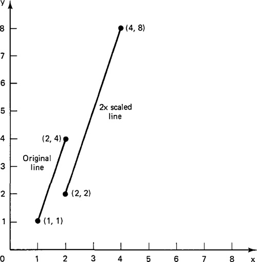
Example 6.2
For the same original line as in Example 6.1, let us apply the scaling factor of 2 to the line. The scaling matrix for the 2 x 2 line definition would therefore be
![]()
The resulting line would be determined by Eq. (6.6) as follows:
![]()
The new line is pictured in Figure 6.4.
Example 6.3
We will again use our same line and rotate the line about the origin by 300. Equation (6.8) would be used to determine the transformed line where the rotation matrix would be:
Figure 6.4 Results of scaling in Example 6.2.
![]()
The new line would be defined as:
![]()
The effect of applying the rotation matrix to the line is shown in Figure 6.5.
Three-dimensional transformations
Transformations by matrix methods can be extended to three-dimensional space. We consider the same three general categories defined in the preceding section. The same general procedures are applied to use these transformations that were defined for the three cases by Eqs. (6.4), (6.6), and (6.8).
TRANSLATION. The translation matrix for a point defined in three dimensions would be
T = (m, n, p) (6.10)
Figure 6.5 Results of rotation in Example 6.3.

and would be applied by adding the increments m, n, and p to the respective coordinates of each of the points defining the three-dimensional geometry element.
SCALING. The scaling transformation is given by
![]()
For equal values of m, n, and p, the scaling is linear.
ROTATION. Rotation in three dimensions can be defined for each of the axes. Rotation about the z axis by an angle θ is accomplished by the matrix
![]()
Rotation about the y axis by the angle θ is accomplished similarly.
![]()
Rotation about the x axis by the angle θ is done with an analogous transformation matrix.
![]()
Concatenation
The previous single transformations can be combined as a sequence of transformations. This is called concatenation, and the combined transformations are called concatenated transformations.
During the editing process when a graphic model is being developed, the use of concatenated transformations is quite common. It would be unusual that only a single transformation would be needed to accomplish a desired manipulation of the image. Two examples of where combinations of transformations would be required would be:
Rotation of the element about an arbitrary point in the element
Magnifying the element but maintaining the location of one of its points in the same location
In the first case, the sequence of transformations would be: translation to the origin, then rotation about the origin, then translation back to the original location. In the second case, the element would be scaled (magnified) followed by a translation to locate the desired point as needed.
The objective of concatenation is to accomplish a series of image manipulations as a single transformation. This allows the concatenated transformation to be defined more concisely and the computation can generally be accomplished more efficiently.
Determining the concatenation of a sequence of single transformations can be fairly straightforward if the transformations are expressed in matrix form as we have done. For example, if we wanted to scale a point by the factor of 2 in a two-dimensional system and then rotate it about the origin by 45°, the concatenation would simply be the product of the two transformation matrices. It is important that the order of matrix multiplication be the same as the order in which the transformations are to be carried out. Concatenation of a series of transformations becomes more complicated when a translation is involved, and we will not consider this case.
Example 6.4
Let us consider the example cited in the text in which a point was to be scaled by a factor of 2 and rotated by 45°. Suppose that the point under consideration was (3, 1). This might be one of several points defining a geometric element. For purposes of illustration let us first accomplish the two transformations sequentially. First, consider the scaling.
Next, the rotation can be performed.
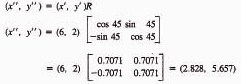
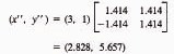
The same result can be accomplished by concatenating the two separate transformation matrices. The product of the two matrices would be
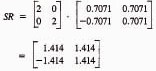
Now, applying this concatenated transformation matrix to the original point, we have
6.6 Data Base Structure and Content
In Section 6.2 the application data base was identified as one of the three modules in the graphics software. Nearly all of the functions of a CAD system depend on its data base. The computer-aided design data base contains the application models, designs, drawings, assemblies, and alphanumeric information such as bills of materials and text. The data base also includes much of the interactive graphics software, such as system commands, function menus, and plotter output routines. The data base resides in computer memory (primary storage) and secondary storage. Since particular parts of the data base can be exchanged readily between primary and secondary storage as needed, we shall not be concerned in this discussion with how the data base is physically stored.
Our principal concern is with the contents of the data base and with its organization. Foley and Van Dam [4] define the basic ingredients of the application model which must be carried in the data base. The following model structure is patterned after their suggested data base organization:
1. Basic graphic elements (points and other elements)
2. Geometry (shape) of the model components and their layout in space
3. Topology or structure of the models—how the various components are connected to form the model
4. Application-specific data, such as material properties
5. Application-specific analysis programs, such as finite-element analysis programs
The list represents a building-block approach to model formulation, with items in category 1 being the most elementary ingredients. They are combined to form the components in category 2, which in turn are used to construct category 3, and so forth. The model structure consists of both data and procedures to connect, describe, and analyze the model.
The model data base can be organized in various ways. This depends on the type of model (mechanical, electrical, etc.) and the preference of the CAD system designer. Some systems lean toward more complete descriptions of the model stored explicitly as data. This requires more storage space. Other systems are designed to store a minimum of data but with more complete procedures so that the model can be recomputed when needed. This saves on storage space, but requires more computation time.
One possible data structure involves storing the coordinates of the geometry, together with other information which might be required to more completely define the model or to use certain application programs (e.g., engineering analysis or numerical control part programming). There are disadvantages to this type of data structure. For example, consider the definition of a cylinder. The definition might consist of a line segment, parallel to the y axis, and rotated about that axis to form the cylinder. The data record for this component would consist of the points for the line segment and an axis of rotation. The computer can generate an image of the cylinder for display purposes, but it does not have all of the solid cylinder data elements stored in the record. It would be difficult for the computer system to determine that the cylinder was a solid object. The characteristic of being solid might be important in a subsequent analysis for interference checking when the cylinder was assembled along with other solid components.
Alternative forms for the data base include the graph-based model. The graph-based model, illustrated in Figure 6.6 for a tetrahedron, is composed of a series of points and lines which establish relationships among the points, edges, and surfaces of the geometric element. Only the points (vertices) are contained as spatial data in the record. However, the relationships that connect edges to vertices, faces to edges, and the solid to faces are also recorded. This turns out to be a compact way to define a solid.
Boolean operations can be used to construct the geometric model. The process is illustrated in Figure 6.7 and is sometimes referred to by the term Boolean modeling. The solid model in part (a) of the figure is formed by the intersection of
Figure 6.6 Graph-based model (b) for a tetrahedron (a).
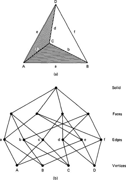
Figure 6.7 Boolean operation C(A + B) performed on elements in (b) to form solid in (a).
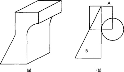
the compliment of the cylinder C with the union of rectangular solid A and triangular prism B. Putting this more concisely, the object in (a) is equal to
C(A + B)
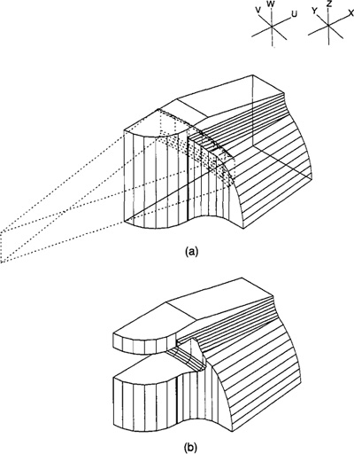
Part (b) of the figure shows the three elements A, B, and C in cross-sectional view. A more complex geometric model, created by similar Boolean operations, is shown in Figure 6.8.
Figure 6.8 Complex geometric solid shape showing removal of material in (a) to form object in (b).(From W. Fitzgerald, F. Gracer, and R. Wolfe, “GRIN: Interactive Graphics for Modeling Solids,” IBM Journal of Research and Development, Vol. 25, No. 4, July, 1981. Copyright 1981 by International Business Machines Corporation; reprinted with permission.)
6.7 Wire-Frame Versus Solid Modeling
The importance of three-dimensional geometry
Early CAD systems were basically automated drafting board systems which displayed a two-dimensional representation of the object being designed. Operators (e.g., the designer or drafter) could use these graphics systems to develop the line drawing the way they wanted it and then obtain a very high quality paper plot of the drawing. By using these systems, the drafting process could be accomplished in less time, and the productivity of the designers could be improved.
However, there was a fundamental shortcoming of these early systems. Although they were able to reproduce high-quality engineering drawings efficiently and quickly, these systems stored in their data files a two-dimensional record of the drawings. The drawings were usually of three-dimensional objects and it was left to the human beings who read these drawings to interpret the three-dimensional shape from the two-dimensional representation. The early CAD systems were not capable of interpreting the three-dimensionality of the object. It was left to the user of the system to make certain that the two-dimensional representation was correct (e.g., hidden lines removed or dashed, etc.), as stored in the data files. More recent computer-aided design systems possess the capability to define objects in three dimensions. This is a powerful feature because it allows the designer to develop a full three-dimensional model of an object in the computer rather than a two-dimensional illustration. The computer can then generate the orthogonal views, perspective drawings, and close-ups of details in the object.
The importance of this three-dimensional capability in interactive computer graphics should not be underestimated. To illustrate the limitations of a two-dimensional line drawing, consider Figure 6.9. It could represent any of a number of possible geometric shapes. Even a three-dimensional perspective drawing, as illustrated in Figure 6.10, does not always uniquely define the solid shape of the object. It is important that the graphics system work with three-dimensional shapes in developing the model of an object.
Wire-Frame models
Most current-day graphics systems use a form of modeling called wire-frame modeling. In the construction of the wire-frame model, the edges of the objects are shown as lines. Figure 4.4 illustrated this form of representation. For objects in which there are curved surfaces, contour lines can be added, as shown in Figure 6.11, to indicate the contour. The image assumes the appearance of a frame constructed out of wire—hence the name “wire-frame“ model.
There are limitations to the models which use the wire-frame approach to form the image. These limitations are, of course, especially pronounced in the case
Figure 6.9 Orthographic views of three-dimensional object without hidden- line removal.
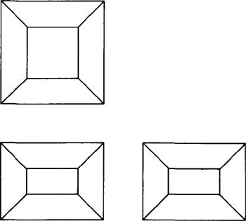
Figure 6.10 Perspective view of three-dimensional object of Figure 6.9 without hidden line removal.
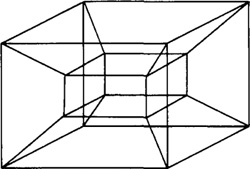
of three-dimensional objects. In many cases, wire-frame models are quite adequate for two-dimensional representation. The most conspicuous limitation is that all of the lines that define the edges (and contoured surfaces) of the model are shown in the image. Many three-dimensional wire-frame systems in use today do not possess an automatic hidden-line removal feature. Consequently, the lines that indicate the edges at the rear of the model show right through the foreground surfaces. This can cause the image to be somewhat confusing to the viewer, and in some cases the image might be interpretable in several different ways (e.g., Figure 6.10). This interpretation problem can be alleviated to some extent through human intervention in removing the hidden background lines in the image.
There are also limitations with the wire-frame models in the way many CAD systems define the model in their data bases. For example, there might be ambiguity in the case of a surface definition as to which side of the surface is solid. This
Figure 6.11 Wireframe model of F/A-18 fighter aircraft, showing primary control curves. (Photo courtesy of McDonnell Douglas Automation Company.)
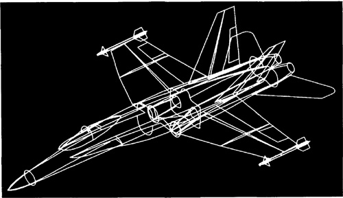
type of limitation prevents the computer system from achieving a comprehensive and unambiguous definition of the object.
Solid models
An improvement over wire-frame models, both in terms of realism to the user and definition to the computer, is the solid modeling approach. In this approach, the models are displayed as solid objects to the viewer, with very little risk of misinterpretation. When color is added to the image, the resulting picture becomes strikingly realistic. Two examples of three-dimensional color solid modeling were shown in Figures 5.9 and 5.10. It is anticipated that graphics systems with this capability will find a wide range of applications outside computer-aided design and manufacturing. These applications will include color illustrations in magazines and technical publications, animation in movie films, and training simulators (e.g., aircraft pilot training).
There are two factors which promote future widespread use of solid modelers (i.e., graphics systems with the capability for solid modeling). The first is the increasing awareness among users of the limitations of wire-frame systems. As powerful as today’s wire-frame-based CAD systems have become, solid model systems represent a dramatic improvement in graphics technology. The second reason is the continuing development of computer hardware and software which make solid modeling possible. Solid modelers require a great deal of computational power, in terms of both speed and memory, in order to operate. The advent of powerful, low-cost minicomputers has supplied the needed capacity to meet this requirement. Developments in software will provide application programs which take advantage of the opportunities offered by solid modelers. Among the possibilities are more highly automated model building and design systems, more complete three-dimensional engineering analysis of the models, including interference checking, automated manufacturing planning, and more realistic production simulation models.
Two basic approaches to the problem of solid modeling have been developed:
1. Constructive solid geometry (CSG or C-rep), also called the building-block approach
3. Boundary representation (B-rep)
The CSG systems allow the user to build the model out of solid graphic primitives, such as rectangular blocks, cubes, spheres, cylinders, and pyramids. This building-block approach is similar to the methods described in Section 6.4 except that a solid three-dimensional representation of the object is produced. The most common method of structuring the solid model in the graphics data base is to use Boolean operations, described in the preceding section and pictured in Figure 6.7.
The boundary representation approach requires the user to draw the outline or boundary of the object on the CRT screen using an electronic tablet and pen or analogous procedure. The user would sketch the various views of the object (front, side, and top, more views if needed), drawing interconnecting lines among the views to establish their relationship. Various transformations and other specialized editing procedures are used to refine the model to the desired shape. The general scheme is illustrated in Figure 6.12.
The two approaches have their relative advantages and disadvantages. The C-rep systems usually have a significant procedural advantage in the initial formulation of the model. It is relatively easy to construct a precise solid model out of regular solid primitives by adding, subtracting, and intersecting the components. The building-block approach also results in a more compact file of the model in the data base.
On the other hand, B-rep systems have their relative advantages. One of them becomes evident when unusual shapes are encountered that would not be included within the available repertoire of the CSG systems. This kind of situation is exemplified by aircraft fuselage and wing shapes and by automobile body styling. Such shapes would be quite difficult to develop with the building-block approach, but the boundary representation method is very feasible for this sort of problem.
Another point of comparison between the two approaches is the difference in the way the model is stored in the data base for the two systems. The CSG approach stores the model by a combination of data and logical procedures (the
Figure 6.12 Input views of the types required for boundary representation (B-rep) approach for solid modeling of object from Figure 6.7.

Boolean model). This generally requires less storage but more computation to reproduce the model and its image. By contrast, the B-rep system stores an explicit definition of the model boundaries. This requires more storage space but does not necessitate nearly the same computation effort to reconstruct the image. A related benefit of the B-rep systems is that it is relatively simple to convert back and forth between a boundary representation and a corresponding wire-frame model. The reason is that the model’s boundary definition is similar to the wire-frame definition, which facilitates conversion of one form to the other. This makes the newer solid B-rep systems compatible with existing CAD systems out in the field.
Because of the relative benefits and weaknesses of the two approaches, hybrid systems have been developed which combine the CSG and B-rep approaches. With these systems, users have the capability to construct the geometric model by either approach, whichever is more appropriate to the particular problem.
6.8 Other CAD Features and CAD/CAM Integration
Most computer-aided design systems currently available offer extensive capabilities for developing engineering drawings. These capabilities include:
1. Automatic crosshatching of surfaces in drawing from wire-frame models.
2. Capability to write text on the drawings. Control can typically be exercised over such parameters as:
Size and style of the lettering
Horizontal and vertical justification of the text
3. Semiautomatic dimensioning. The dimensions can be obtained from the data base. Dimensioning features typically include:
Linear or angular conventions, depending on which is more appropriate
English and/or metric (International System)
Dimensions displayed in decimal or fractional notation
Various types of tolerance displays
4. Automatic generation of bill of materials (assembly and materials listings).
All of these features are helpful in reducing the time required to complete the design and drafting process.
In most CAD systems, an interface is generally provided to various high-level programming languages such as FORTRAN. This interface allows the development of application programs for analysis purposes. It also provides the opportunity to utilize programs and routines written at other facilities. This interface allows a wide variety of powerful design analysis and manufacturing planning procedures to be applied to the product development.
Experience has demonstrated that the benefits obtained from an integrated CAD/CAM data base are far greater than those which can be realized from applying CAD and CAM as separate technologies. There is a significant overlap in the data base required for design and that which is required for manufacturing. Bridging the gap that has traditionally existed between design and manufacturing is a critical objective of CAD/CAM.
Much of the remainder of this book will be concerned with topics in computer-aided manufacturing. However, it is important to recognize that in most of the topics discussed, the degree to which computerized automation can be achieved, and the success of the application, relies heavily on the generation of the data base during computer-aided design.
References
[1] BOYSE, J. W., AND GILCHRIST, J. E., “GM Solid: Interactive Modeling for Design and Analysis of Solids,” IEEE Computer Graphics, March, 1982, pp. 27–40.
[2] CHASEN, S. H., Geometric Principles and Procedures for Computer Graphic Applications, Prentice-Hall, Inc., Englewood Cliffs, N.J., 1978.
[3] FITZGERALD, W., GRACER, P., and WOLFE, R., “GRIN: Interactive Graphics for Modeling Solids,” IBM Journal of Research and Development, July, 1981, pp. 281–294.
[4] FOLEY, J. D., AND VAN DAM, A., Fundamentals of Interactive Computer Graphics, Addison-Wesley Publishing Co., Inc., Reading, Mass., 1982.
[5] GLLOL, W. K., Interactive Computer Graphics, Prentice-Hall, Inc., Englewood Cliffs, N.J., 1978.
[6] KLNNUCAN, P., “Solid Modelers Make the Scene,” High Technology, July/August, 1982, pp. 38–44.
[7] MYERS, W., “An Industrial Perspective on Solid Modeling,” IEEE Computer Graphics, March, 1982, pp. 86–97.
[8] NEWMAN, W. M., AND SPROULL, R. F., Principles of Interactive Computer Graphics, 2nd ed., McGraw-Hill Book Company, New York, 1979.
[9] REQUICHA, A. A. G., AND VOELCKER, H. B., “Solid Modeling: A Historical Summary and Contemporary Assessment,” IEEE Computer Graphics, March, 1982, pp. 9–24.
[10] ROGERS, D. F., AND ADAMS, J. A., Mathematical Elements in Computer Graphics, McGraw-Hill Book Company, New York, 1976.
[11] ZIMMERS, E. W., JR., Computer-Aided Design Module, General Electric CAD/CAM Seminar, Lehigh University, Bethlehem, Pa., 1982.
Problems
6.1. Figures 6.9 and 6.10 show a wire-frame drawing of a three-dimensional solid object. However, there are several possible interpretations of this drawing. Make a list of as many interpretations as you can think of.
6.2. Make a sketch of two or three solid primitives (such as a rectangular solid) and show how these various primitives can be scaled, reoriented, added, subtracted, and intersected to create the geometry of the object in Figure 6.10.
6.3. A line is defined by its end points (0, 0) and (2, 3) in a two-dimensional graphics system. Express the line in matrix notation and perform the following transformations on this line:
(a) Scale the line by a factor of 2.0.
(b) Scale the original line by a factor of 3.0 in the x direction and 2.0 in the y direction.
(c) Translate the original line by 2.0 units in the x direction and 2.0 units in the y direction.
(d) Rotate the original line by 45° about the origin.
(e) Plot the original line and each of the four transformations on a piece of graph paper.
6.4. A triangle is defined in a two-dimensional ICG system by its vertices (0, 2), (0, 3), and (1,2). Perform the following transformations on this triangle:
(a) Translate the triangle in space by 2 units in the x direction and 5 units in the y direction.
(b) Scale the original triangle by a factor of 1.5.
(c) Scale the original triangle by a factor of 1.5 in the x direction and 3.0 in the y direction.
(d) Rotate the original triangle by 45° about the origin.
6.5. A line is defined in two-dimensional space by its end points (1,2) and (6, 4). Express this in matrix notation and perform the following transformations in succession on this line:
(a) Rotate the line by 90° about the origin.
(b) Scale the line by a factor of 1/2.
(c) Show the sequence of transformations on a piece of graph paper.
6.6 Determine the concatenation of the transformations performed in Problem 6.5. It should be expressed in matrix notation.
6.7. A cube is defined in three-dimensional space with edges which are one unit in length. The comers of the cube are located at (0, 0, 0), (0, 0, 1), (0, 1, 0,), (0, 1, 1), (1, 0, 0), (1, 0, 1), (1, 1, 0), (1, 1, 1). Determine the locations of the corners if the cube is first translated by 2.0 units in the x direction and then scaled by a factor of 3.0.
6.8. Using the same cube from Problem 6.7, carry out the two transformations indicated in that problem in the reverse order. Are the resulting cube and its position the same as in Problem 6.7?
6.9. Rotate the cube from Problem 6.7 about the y axis by an angle of 45°.
6.10. A line in two-dimensional space has end points defined by (1, 1) and (1, 3). It is desired to move this line by a series of transformations so that its end points will be at (0, 1) and (0, 5).
(a) Describe the sequence of transformations required to accomplish the movement of the line as specified.
(b) For each transformation in the sequence, write the transformation matrix.
6.11. A point in two dimensions is located at (3,4). It is desired to relocate the point by means of rotation and scaling transformations only (no translation) to a new position defined by (0, 8).
(a) Describe the sequence of transformations required to accomplish the movement of the line as specified.
(b) Write the transformation matrix for each step in the sequence.
(c) Write the concatenated transformation matrix for the sequence.
6.12. In order to perform the translation transformation in two dimensions, the transformation must be represented by a 3 x 3 matrix. In order to be compatible, the representation of a point would be given as (x, y, 1). This n + 1 component vector for n- dimensional space is called a homogeneous coordinate representation. Thus, for translating a point, the homogeneous representation would be
![]()
where n and m in the 3 X 3 translation matrix represent the displacement in the x and y directions, respectively.
(a) Use the equation above to translate the point at (1, 1) in the x direction by 2 units and hi the y direction by 5 units.
(b) Develop the analogous equation for the translation of a line, and translate the line whose matrix is
![]()
by 3 units in the x direction.