Chapter 15
Inventory Management and MRP

15.1 Introduction

Chapter 14 provided a general description of a modern computer-integrated production management system (CIPMS). One of the most important components of the CIPMS is the material requirements planning system. MRP is sometimes thought of as an inventory management system. In this chapter we describe material requirements planning, its underlying concepts, how it works, and its benefits. Entire books have been written on this subject, for example, [5]. The interested reader is invited to explore the many facets of MRP in that volume, details of which are beyond the scope of our book on CAD/CAM.

MRP has expanded to mean more than material requirements planning. Wight [10] is using the term “MRP II” to represent manufacturing resource planning, a system for planning and controlling the operational, engineering, and financial resources of a manufacturing firm. We shall examine MRP II later. We begin the chapter with a general introduction to inventory management.

15.2 Inventory Management

Inventory control is concerned with achieving an optimum balance between two competing objectives. The objectives are first, to minimize investment in inventory, and second, to maximize the service levels to the firm’s customers and its own operating departments. The purpose of this section is not to provide a comprehensive discussion of the theory and methods by which these objectives are achieved. For that purpose, the reader is referred to any of several books in the field, for example, Peterson and Silver [6]. Instead, our purpose is to describe how inventory control is accomplished in a modern computer-integrated production management system.

Inventory types and general control procedures

There are four types of inventory with which a manufacturing firm must concern itself:

1. Raw materials and purchased components. These are the basic materials out of which the product and components are made. Purchased components are similar to raw materials. The difference is that the supplier does all of or a portion of the processing on the component.

2. In-process inventory. After processing begins on the raw materials or purchased components, there is a time lapse (the manufacturing lead time) before the processing has been completed. During that time, the materials are in-process.

3. Finished product. The finished product may be stored in the factory or warehouse before shipment to the customer. This category includes service parts as well as end product.

4. Maintenance, repair, and tooling inventories. These are the cutting tools and fixtures used to operate the machines in the factory and the repair parts needed to fix the machines when they break down. Electrical spare parts and plumbing supplies also fit into this category.

To manage these various kinds of inventories, two alternative control procedures can be used:

1. Order point systems. This has been the traditional approach to inventory control. In these systems, the items are restocked when the inventory levels become low.

2. Material requirements planning. MRP is sometimes thought of as an inventory control procedure. It is really more than that, as we shall see.

It is important that the proper control procedure be applied to each of the four types of inventory. In general, MRP is the appropriate control procedure for inventory types 1 and 2 (raw materials, purchased components, and in-process inventory). Order point systems are often considered the appropriate procedure to control inventory types 3 and 4 (finished product, maintenance and repair parts, and tooling). In some cases, order point systems may be applied for certain widely used raw materials and purchased components.

Order point systems

Order point systems are concerned with the two related problems of determining when to order and how much to order. Determining when to order is often accomplished by establishing a “reorder point.” When the inventory level for a particular item falls to the reorder point, it is time to restock the item. A computerized inventory control system can be programmed to track the inventory level continuously as transactions are entered against existing stocks. It automatically indicates when it is time to reorder, perhaps even generating a purchase requisition to do so.

The problem of determining how much to order is typically based on the use of the familiar economic order quantity (EOQ) formula, which states

where EOQ = quantity of the item to be ordered

D = annual demand rate for the item

S = setup cost or ordering cost per order

H = annual holding cost for the item to be carried in inventory

Example 15.1

The EOQ formula might be quite appropriate for controlling inventory on certain tooling items. Suppose that we wanted to use the formula [Eq. (15.1)], to determine the order quantity for a particular drill bit that is used in the shop. The annual usage rate (demand rate) for the drill is 8000 units per year. The cost to place an order, including the vendor’s setup charge, is $100. And the holding cost for us to carry the drill in inventory is figured at $1.60 per drill each year. The holding cost would typically be calculated by applying an interest rate to the unit cost of the item. For example, if the interest rate were 20% and the drill cost $8.00 per unit, the holding cost would be 0.20 X 8.00 = $1.60 per drill per year.

Using these values in the EOQ equation, we get

EOQ = 1000 units per order

Each time an order is placed, it is most economical to order 1000 units.

Computer software can be written to perform this economic order quantity calculation for all the items stocked in inventory. The program keeps track of usage or demand rates for the items in stock and computes the term D in Eq. (15.1). Up-to-date files are maintained by the system on current stock levels so that when inventory falls below the reorder point, a new order for the optimum order quantity can be issued. Problem 15.2 at the end of the chapter deals with such a program.

The inventory management module

The inventory management module of the computer-integrated production management system would be organized to accomplsih two major functions:

1. Inventory accounting

2. Inventory planning and control

Both of these functions apply to all types of inventories (raw materials, in-process inventories, finished product, and maintenance and tooling items).

INVENTORY ACCOUNTING. Inventory accounting is concerned with inventory transactions and inventory records. The accuracy and completeness of these transactions and records is critical to the success of the CIPMS. Material requirements planning, for example, depends on accurate inventory records to perform its planning function.

Inventory transactions include receipts, disbursements or issues, returns, and loans (e.g., the loaning of a tool or fixture that would be returned after use). Inventory transactions would also allow for adjustments to be made in the records as a result of a physical inventory count. The various changes would be entered by means of a terminal located at the site of the transaction (in the receiving department, raw material stores, tool crib, etc.).

The purpose of entering the various transactions is to maintain accurate inventory records. Additions and subtractions are made to the inventory balance as a result of the transactions. The term “item master file” is sometimes used to describe the computerized inventory record file. The types of data contained in the

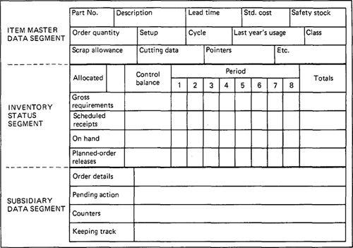
Figure 15.1 Record of an inventory item. (Reprinted with permission from Orlicky [5].)

record for a given item would typically include the categories shown in Figure 15.1. The file contains three segments:

1. Item master data segment

2. Inventory status segment

3. Subsidiary data segment

The first segment gives the item’s identification (by part number) and other data, such as lead time, cost, and order quantity. The second segment (inventory status segment) provides a time-phased record of inventory status. In MRP it is important to know not only the current level of inventory, but also the future changes that will occur against the inventory status. Therefore, the inventory status segment lists the gross requirements for the item, scheduled receipts, on-hand status, and planned-order releases. The third file segment (subsidiary data segment) contains miscellaneous information pertaining to purchase orders, scrap or rejects, engineering change actions, and so on.

INVENTORY PLANNING AND CONTROL. In addition to maintaining an accurate item master file, the inventory management module must also be concerned with the planning and control of inventories. Many of these planning and control activities are accomplished by the MRP module. Other functions include:

Determining economic lot sizes

Determining safety stock levels

Determining ordering policies and reorder points

ABC inventory analysis

Analysis of usage rates for lot size calculations and other purposes

Automatic generation of requisitions for purchasing

In these and other inventory planning functions, the purpose is to keep inventory investment as low as possible while achieving a satisfactory service level. The inventory management module would accomplish some of these functions automatically, without human intervention. In other cases where human judgment is required, the proper information would be provided to the decision maker for appropriate action.

15.3 Material Requirements Planning

Material requirements planning is a computational technique that converts the master schedule for end products into a detailed schedule for the raw materials and components used in the end products. The detailed schedule identifies the quantities of each raw material and component item. It also tells when each item must be ordered and delivered so as to meet the master schedule for the final products.

MRP is often considered to be a subset of inventory control. While it is an effective tool for minimizing unnecessary inventory investment, MRP is also useful in production scheduling and purchasing of materials.

The concept of MRP is relatively straightforward. What complicates the application of the technique is the sheer magnitude of the data to be processed. The master schedule provides the overall production plan for final products in terms of month-by-month or week-by-week delivery requirements. Each of the products may contain hundreds of individual components. These components are produced out of raw materials, some of which are common among the components. For example, several parts may be produced out of the same sheet steel. The components are assembled into simple subassemblies. Then these subassemblies are put together into more complex assemblies—and so forth, until the final product is assembled together. Each production and assembly step takes time. All of these factors must be incorporated into the MRP computations. Although each separate computation is uncomplicated, the magnitude of all the data to be processed is so large that the application of MRP is virtually impossible unless carried out on a digital computer.

15.4 Basic MRP Concepts

Material requirements planning is based on several basic concepts which are implicit in the preceding description but not explicitly defined. These concepts are:

1. Independent versus dependent demand

2. Lumpy demand

3. Lead times

4. Common use items

Independent versus dependent demand

This distinction is fundamental to MRP. Independent demand means that demand for a product is unrelated to demand for other items. End products and spare parts are examples of items whose demand is independent. Independent demand patterns must usually be forecasted.

Dependent demand means that demand for the item is related directly to the demand for some other product. The dependency usually derives from the fact that the item is a component of the other product. Not only component parts, but also raw materials and subassemblies, are examples of items that are subject to dependent demand.

Whereas demand for the firm’s end products must often be forecasted, the raw materials and component parts should not be forecasted. Once the delivery schedule for the end products is established, the requirements for components and raw materials can be calculated directly. For example, even though the demand for automobiles in a given month can only be forecasted, once that quantity is established we know that four regular tires will be needed to deliver the car plus one spare tire.

MRP is the appropriate technique for determining quantities of dependent demand items. These items constitute the inventory of manufacturing: raw materials, work-in-progress, component parts, and subassemblies. Accordingly, MRP is a very powerful tool in the planning and control of manufacturing inventories.

Lumpy demand

In an order point system, the assumption is generally made that the demand for the item in inventory will occur at a gradual, continuous rate. This assumption is important for developing the mathematical model to derive the economic lot size formula. In a manufacturing situation, demand for the raw materials and components of a product will occur in large increments rather than in small, almost continuous units. The large increments correspond to the quantities needed to make a certain batch of the final product. When the demand occurs in these large steps, it is referred to by the term “lumpy demand.” MRP is the appropriate approach for dealing with inventory situations characterized by lumpy demand.

Lead times

The lead time for a job is the time that must be allowed to complete the job from start to finish. In manufacturing there are two kinds of lead times: ordering lead times and manufacturing lead times. An ordering lead time for an item is the time required from initiation of the purchase requisition to receipt of the item from the vendor. If the item is a raw material that is stocked by the vendor, the ordering lead time should be relatively short, perhaps a few weeks. If the item must be fabricated by the vendor, the lead time may be substantial, perhaps several months.

Manufacturing lead time is the time needed to process the part through the sequence of machines specified on the route sheet. It includes not only the operation times but also the nonproductive time that must be allowed.

In MRP, lead times are used to determine starting dates for assembling final products and subassemblies, for producing component parts, and for ordering raw materials.

Common use items

In manufacturing, the basic raw materials are often used to produce more than one component type. Also, a given component may be used on more than one final product. For example, the same type of steel rod stock may be used to produce screws on an automatic screw machine. Each of the screw types may then be used on several different products. MRP collects these common-use items from different products to effect economies in ordering the raw materials and manufacturing the components.

15.5 Inputs to MRP

MRP converts the master production schedule into the detailed schedule for raw materials and components. For the MRP program to perform this function, it must operate on the data contained in the master schedule. However, this is only one of three sources of input data on which MRP relies. The three inputs to MRP are:

1. The master production schedule and other order data

2. The bill-of-materials file, which defines the product structure

3. The inventory record file

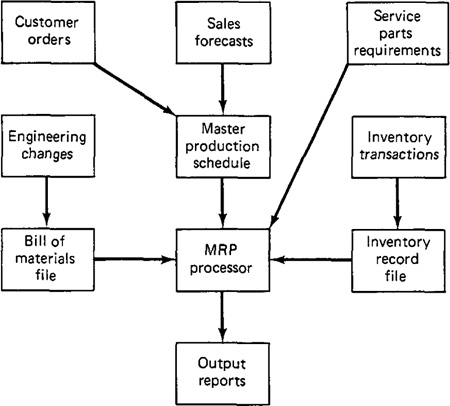
Figure 15.2 Structure of a material requirements planning (MRP) system.

Figure 15.2 presents a diagram showing the flow of data into the MRP processor and its conversion into useful output reports. The three inputs are described in the sections below.

Master production schedule

As explained in Chapter 14, the master production schedule is a list of what end products are to be produced, how many of each product is to be produced, and when the products are to be ready for shipment. The general format of a master production schedule is illustrated in Figure 15.3. Manufacturing firms generally work toward monthly delivery schedules. However, in Figure 15.3, the master schedule uses weeks as the time periods (for purposes of an example that will be developed later). The master schedule must be based on an accurate estimate of demand for the firm’s product, together with a realistic assessment of its production capacity.

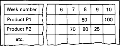
Figure 15.3 Master production schedule for products P1 and P2, showing week delivery quantities.

Product demand that makes up the master schedule can be separated into three categories. The first consists of firm customer orders for specific products. These orders usually include a specific delivery date which has been promised to the customer by the sales department. The second category is forecasted demand. Based on statistical techniques applied to past demand, estimates provided by the sales staff, and other sources, the firm will generate a forecast of demand for its various product lines. This forecast may constitute the major portion of the master schedule. The third category is demand for individual component parts. These components will be used as repair parts and are stocked by the firm’s service department. This third category is often excluded from the master schedule since it does not represent demand for end products. In Figure 15.2 we show it as feeding directly into the MRP processor.

Bill of materials file

In order to compute the raw material and component requirements for end products listed in the master schedule, the product structure must be known. This is specified by the bill of materials, which is a listing of component parts and subassemblies that make up each product. Putting all these assembly lists together, we have the bill-of-materials file (BOM).

The structure of an assembled product can be pictured as shown in Figure 15.4. This is a relatively simple product in which a group of individual components make up two subassemblies, which in turn make up the product. The product structure is in the form of a pyramid, with lower levels feeding into the levels above. We can envision one level below that shown in Figure 15.4. This would consist of the raw materials used to make the individual components. The items at each successively higher level are called the parents of the items in the level directly below. For example, subassembly S1 is the parent of components C1, C2, and C3. Product P1 is the parent of subassemblies S1 and S2.

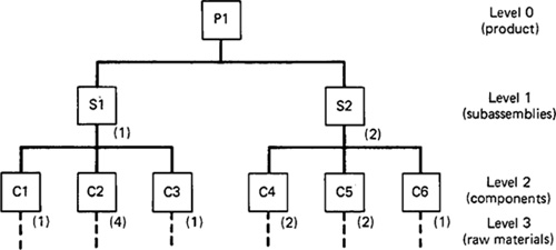
Figure 15.4 Product structure for product P1.

The product structure must also specify how many of each item are included in its parent. This is accomplished in Figure 15.4 by the number in parentheses to the right and below each block. For example, subassembly S1 contains four of component C2 and one each of components C1 and C3.

Inventory record file

It is mandatory in material requirements planning to have accurate current data on inventory status. This is accomplished by utilizing a computerized inventory system which maintains the inventory record file or item master file. The features of such a system were discussed in Section 15.2 and illustrated in Figure 15.1.

A definition of the lead time for the raw materials, components, and assemblies must be established in the inventory record file. The ordering lead time can be determined from purchasing records. The manufacturing lead time can be determined from the process route sheets (or routing file).

It is important that the inputs to the MRP processor be kept current. The bill-of-materials file must be maintained by feeding any engineering changes that affect the product structure into the BOM. Similarly, the inventory record file is maintained by inputing the inventory transactions to the file.

15.6 How MRP Works

The material requirements planning processor operates on the data contained in the master schedule, the bill-of-materials file, and the inventory record file. The master schedule specifies a period-by-period list of final products required. The BOM defines what materials and components are needed for each product. The inventory record file contains information on the current and future inventory status of each component. The MRP program computes how many of each component and raw material are needed by “exploding” the end-product requirements into successively lower levels in the product structure. Referring to the master schedule in Figure 15.3, 50 units of product P1 are specified in the master schedule for week 8. Now referring to the product structure in Figure 15.4, 50 units of P1 explode into 50 units of subassembly S1 and 100 units of S2, and the following numbers of units for the components:

C1: 50units

C2: 200 units

C3: 50 units

C4: 200 units

C5: 200 units

C6: 100 units

The quantities of raw materials for these components would be determined in a similar manner.

There are several factors that must be considered in the MRP parts and materials explosion. First, the component and subassembly quantities given above are gross requirements. Quantities of some of the components and subassemblies may already be in stock or on order. Hence the quantities that are in inventory or scheduled for delivery in the near future must be subtracted from gross requirements to determine net requirements for meeting the master schedule.

A second factor in the MRP computations is manifested in the form of lead times: ordering lead times and manufacturing lead times. The MRP processor must determine when to start assembling the subassemblies by offsetting the due dates for these items by their respective manufacturing lead times. Similarly, the component due dates must be offset by their manufacturing lead times. Finally, the raw materials for the components must be offset by their respective ordering lead times. The material requirements planning program performs this lead-time-offset calculation from data contained in the inventory record file and from route sheet data.

A third factor that complicates MRP is common-use items. Some components and many raw materials are common to several products. The MRP processor must collect these common use items during the parts explosion. The total quantities for each common use item are then combined into a single net requirement for the item.

Finally, a feature of MRP that should be emphasized is that the master production schedule provides time-phased delivery requirements for the end products, and this time phasing must be carried through the calculations of the individual component and raw material requirements.

Example 15.2

To illustrate how MRP works, let us consider the requirements planning procedure for one of the components of product P1. The component we will consider is C4. This part happens to be used also on one other product: P2 (see the master schedule of Figure 15.3). However, only one of item C4 is used on each P2 produced. The product structure of P2 is given in Figure 15.5. Component C4 is made out of raw material M4. One unit of M4 is needed to produce a unit of C4. The ordering and manufacturing lead times needed to make the MRP computations are as follows:

P1: assembly lead time = 1 week

P2: assembly lead time = 1 week

S2: assembly lead time = 1 week

S3: assembly lead time = 1 week

C4: manufacturing lead time = 2 weeks

M4: ordering lead time = 3 weeks

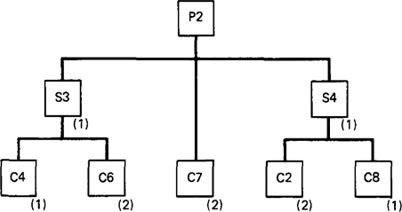
Figure 15.5 Product structure for product P2.

Figure 15.6 Initial inventory status of material M4 in Example 15.2.

The current inventory and order status of item M4 is shown in Figure 15.6. There are no stocks or orders for any of the other items listed above.

The solution is presented in Figure 15.7. The delivery requirements for products P1 and P2 must be offset by the 1-week assembly lead time to obtain the planned order releases. Since the subassemblies to make the products must be ready, these order release quantities are “exploded” into requirements for subassemblies S2 (for P1) and S3 (for P2). These net requirements are then offset by the 1-week lead time and combined (in week 6) to obtain the gross requirements for part C4. Net requirements are equal to gross requirements for P1, P2, S2, S3, and C4 because of no on-hand inventory and no planned orders. We see the effect of current and planned stocks in the time-phased inventory picture for M4. The on-hand stock of 50 plus the scheduled receipts of 40 are used to meet the gross requirements of 70 units of M4 in week 3. Twenty units remain after meeting these requirements, which can be applied to the gross requirements of 280 units of M4 in week 4. Net requirements in week 4 are therefore 280 - 20 = 260 units. With an ordering lead time of 3 weeks, the order release for the 260 units must be planned for week 1.

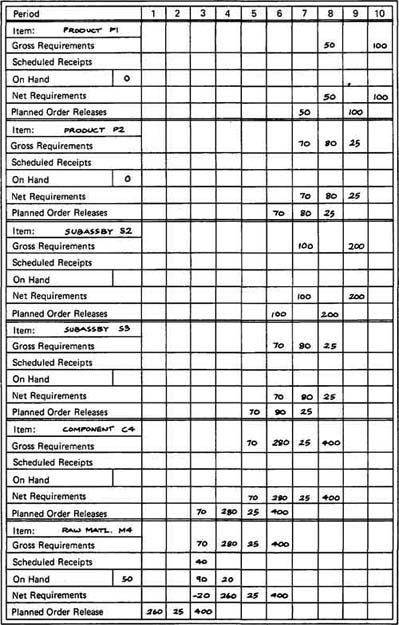
Figure 15.7 MRP solution for Example 15.2.

15.7 MRP Output Reports

The material requirements planning program generates a variety of outputs that can be used in the planning and management of plant operations. These outputs include:

1. Order release notice, to place orders that have been planned by the MRP system

2. Reports showing planned orders to be released in future periods

3. Rescheduling notices, indicating changes in due dates for open orders

4. Cancellation notices, indicating cancellation of open orders because of changes in the master schedule

5. Reports on inventory status

The outputs of the MRP system listed above are called primary outputs by Orlicky [5]. In addition, secondary output reports can be generated by the MRP system at the user’s option. These reports include:

1. Performance reports of various types, indicating costs, item usage, actual versus planned lead times, and other measures of performance

2. Exception reports, showing deviations from schedule, orders that are overdue, scrap, and so on

3. Inventory forecasts, indicating projected inventory levels (both aggregate inventory as well as item inventory) in future periods

15.8 Benefits of MRP

There are many advantages claimed for a well-designed, well-managed material requirements planning system. Among these benefits reported by MRP users are the following. The statistical data are compiled from Schaffer [8].

Reduction in inventory. MRP mainly affects raw materials, purchased components, and work-in-process inventories. Users claim a 30 to 50% reduction in work-in-process.

Improved customer service. Some MRP proponents claim that late orders are reduced 90%.

Quicker response to changes in demand and in the master schedule.

Greater productivity. Claims are that productivity can be increased by 5 to 30% through MRP. Labor requirements are reduced correspondingly.

Reduced setup and product changeover costs.

Better machine utilization.

Increased sales and reductions in sales price. These are also claimed as MRP benefits by some users.

As a result of the recognition given to these benefits in trade journals and professional societies, applications of material requirements planning have grown dramatically since the late 1960s. Today, more and more manufacturing firms of any significant size either use a computerized MRP system or are planning to implement one.

15.9 MRP II: Manufacturing Resource Planning

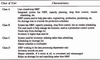
In his book on manufacturing resource planning, Wight [10] defines four classes of MRP users. The characteristics of the four classes are listed in Table 15.1. The lowest level is class D, in which the potential utility of material requirements planning is hardly realized at all. MRP is used basically as a data processing system with many of the traditional production control procedures (e.g., shortage lists, expediting) still being used. At the top of the list is the class A MRP user. This is a company that uses material requirements planning together with capacity planning, shop floor control, and other components of a computer-integrated production management system. The next step beyond the class A user is MRP II. To describe MRP II, let us first examine the progressive evolution of material requirements planning into manufacturing resource planning.

Table 15.1 Four Classes of MRP Users

Four steps of MRP

Material requirements planning has changed significantly over the years. Four steps can be identified in the evolution of MRP [10]:

1. An improved ordering method

2. Priority planning

3. Closed-loop MRP

4. MRP II

The first step was implemented when initial use of the computer was made to perform the requirements planning calculations. Before the computer, this task was performed manually and consumed tremendous amounts of time and manpower to accomplish. Computerized MRP systems represented a tremendous improvement in the ordering of raw materials and components because of the speed and accuracy with which the requirements planning task could be performed.

The need for the second step in MRP evolution grew out of attempts to implement step one MRP in conjunction with an unrealistic master schedule. This was a master schedule that ignored the limitation imposed by plant capacity and other constraints. It caused the MRP processor to generate schedules and requirements that could not be accomplished by the factory. As a result, the use of shortage lists continued. To overcome these problems, the MRP systems began to incorporate priority planning into their computations. The term “priority planning” connotes an MRP system which determines not only what materials should be ordered but also when those materials will be required. The planning of material requirements can be phased into time periods (weeks, or even days). Priority planning not only provides a means for dealing with rush jobs by increasing their priorities; it also helps to unexpedite jobs whose priorities have been reduced.

Step three MRP represents the level of achievement of the class A MRP user. Closed-loop MRP is an improvement over step two MRP because it not only plans the priorities but also provides feedback information relative to executing the priority plan. Closed-loop MRP means that the various functions in production planning and control (capacity planning, inventory management, shop floor control, and MRP in Figure 14.2) have been integrated into a single system. It also means that there is feedback from vendors, the production shop, and so on, when problems arise in implementing the production plan.

MRP II

Closed-loop MRP represents a significant achievement in terms of tieing together the various separate functions of a production planning and control system. However, there is one final step in the evolution of MRP (at least, as it is currently conceived). This fourth step involves a link-up between the closed-loop MRP system and the financial systems of the company. Manufacturing resource planning is the name given to this combination.

MRP II possesses two basic characteristics which go beyond closed-loop MRP:

1. It is an operational and financial system.

2. It is a simulator.

The operational and financial system makes MRP II a company-wide system, concerned with all facets of the business, including sales, production, engineering, inventories, and cash flows. In all cases, the operations of the individual departments are reduced to the same common denominator: financial data. This common base provides the company management with the information needed to manage it successfully. For example, raw materials on hand can be converted into their equivalent cost and summed over all stocks in inventory. Work-in-process can be evaluated by adding raw material costs to the cost of labor turned in against the particular part numbers and orders. Other operating data can be expressed in money terms by a similar calculation procedure.

MRP II is also a simulator which is intended to answer “what if” questions. The simulator can be used to simulate the probable outcomes of alternative production plans and management decisions which are under consideration.

In essence, manufacturing resource planning is quite similar to the general model of a computer-integrated production management system described in Chapter 14. The CIPMS includes not only the operational system (MRP, inventory management, capacity planning, etc.) but also the cost planning and control module. This cost planning and control module is the connection with the company’s accounting and financial systems.

References

[1] CHASE, R., AND AQUILANO, N., Production and Operations Management, 3rd ed., Richard D. Irwin, Inc., Homewood, Ill., 1981, Chapter 16.

[2]GROOVER, M. P., Automation, Production Systems, and Computer-Aided Manufacturing, Prentice-Hall, Inc., Englewood Cliffs, N.J., 1980, Chapter 17.

[3] HALEVI, G., The Role of Computers in Manufacturing Processes, John Wiley & Sons, Inc., New York, 1980.

[4] INTERNATIONAL BUSINESS MACHINES CORPORATION, Communications Oriented Production Information and Control System, Publication G320-1974.

[5] ORUCKY, J., Material Requirements Planning, McGraw-Hill Book Company, New York, 1975.

[6] PETERSON, R., AND SILVER, E. A., Decision Systems for Inventory Management and Production Planning, John Wiley & Sons, Inc., New York, 1979.

[7] PLOSSL, G. W., “MRP Yesterday, Today, and Tomorrow,” Production and Inventory Management, Third Quarter, 1980, pp. 1–10.

[8] SCHAFFER, G. H., “Implementing CIM,” American Machinist, August, 1981, pp. 151–174.

[9] WIGHT, O. W., Production and Inventory Management in the Computer Age, Cahners Books, Boston, 1974.

[10] WIGHT, O. W. MRP II: Unlocking America’s Productivity Potential, Oliver Wight Limited Publications, Inc., Williston, Vt., 1981.

Problems

15.1. The monthly usage rate for a certain type of cemented carbide insert used in the machine shop is averaging 1100 units. The inserts cost $4.36 each when ordered in quantities over 500. It is estimated that it costs an average of $60 each time a batch of inserts is ordered. The holding cost for this shop is based on using 25% per year of the cost of the item in inventory. What is the economic order quantity for this insert?

15.2. Develop a computer program for an automated inventory control and reordering system. The program should have the following capabilities and specifications:

(a) It should maintain records for 200 items in inventory.

(b) It must have a reorder point for each item.

(c) It should calculate the usage rate (demand rate) for each item when the reorder point is reached.

(d) It should compute the EOQ by Eq. (15.1). Assume that the annual holding cost and ordering cost are known for each item.

15.3. Using the master schedule of Figure 15.2 and the product structures in Figures 15.3 and 15.5, determine the time-phased requirements for component C6. The raw material used in component C6 is M6. Two units of C6 are obtained from every unit of M6. Lead times are as follows:

P1: assembly lead time = 1 week

P2: assembly lead time = 1 week

S2: assembly lead time = 1 week

S3: assembly lead time = 1 week

C6: manufacturing lead time = 2 weeks

M6: ordering lead time = 2 weeks

Assume that the current inventory status for all of the items above is: units on hand = 0, units on order = 0. The format of the solution should be similar to that presented in Example 15.1.

15.4. Solve Problem 15.3 if the current inventory and order status for S3, C6, and M6 is:

S3: inventory on hand = 2, on order = 0

C6: inventory on hand = 5, on order = 10 due for delivery in week 2

M6: inventory on hand = 10, on order = 50 due for delivery in week 2

15.5. Product P4 is assembled out of 2 units of S5 and 1 unit of S6. Both S5 and S6 are subassemblies. S5 is made of 1 unit of C2, 2 units of C3, and 4 units of C4. S6 is made of 3 units of C3 and 1 unit of C5. Draw a diagram of the product P4 structure similar to the format of Figure 15.3.

15.6. This problem makes use of the data for product P4 in Problem 15.5. The master schedule specifies that 100 units of P4 are to be delivered in week 10, 150 units in week 11, and 200 units in weeks 12, 13, and 14. The lead times for each item are given as follows:

P4: assembly lead time = 2 weeks

S5: assembly lead time = 1 week

S6: assembly lead time = 1 week

C2: ordering lead time = 3 weeks

C3: ordering lead time = 4 weeks

C4: ordering lead time = 2 weeks

C5: ordering lead time = 3 weeks

Assume that the current inventory status for these items is: units on hand = 0, units on order = 0. Also assume that these components and subassemblies are not common-use items on any other products.

Develop a computer program to compute the time-phased gross and net requirements and planned order release dates for the data of this problem. The output format should be similar to that shown in Figure 15.6. The planning horizon should cover weeks 1 through 14 for all components, subassemblies, and the final product P4.