
Chapter 16
Shop Floor Control and Computer Process Monitoring
16.1 Introduction
Production management systems are concerned with two related objectives: planning, and control of the manufacturing operations. The functions of production planning, development of the master schedule, capacity planning, and MRP all deal with the planning objective. In this chapter we consider the control objective. Systems that accomplish this objective are often referred to by the term “shop floor control” (SFC).
At the time of this writing, the techniques of shop floor control are in the midst of a transition from manual methods to computerized methods. Shop floor control has been recognized as a distinct problem area in production management for many years. In 1973, the American Production and Inventory Control Society published a book entitled Shop Floor Controls [1]. At that time computer and data collection hardware for SFC was not nearly as well developed as it is today. Even today, this area must be considered as one which is rapidly changing both in terms of hardware and in terms of theory. What we attempt to present is the latest practice in computerized shop floor control systems. This includes systems that establish a direct connection between the computer and the manufacturing process for the purpose of monitoring the operation.
16.2 Functions of Shop Floor Control
Production managers are faced with the problem of acquiring up-to-date information on the progress of orders in the factory and making use of that information to control factory operations. This is the problem addressed by a shop floor control system. The functions of a shop floor control system are classifed by Raffish [17] as follows:
1. Priority control and assignment of shop orders.
2. Maintain information on work-in-process for MRP.
3. Monitor shop order status information.
4. Provide production output data for capacity control purposes.
These functions are explained in the following subsections. The reader should refer back to Figure 14.2 to recall the relationships and lines of communication between shop floor control and the other functions (MRP, capacity planning, etc.) in a computer-integrated production management system.
Priority control and assigment of shop orders
MRP and priority planning are concerned with the time-phased planning of materials, work-in-process, and assembly of final product. Priority control can be considered as the execution phase of this planning process. Priority control is concerned with maintaining the appropriate priorities for work-in-process in response to changes in job order status. Suppose that the delivery date requirement for one batch of product was moved forward because demand for the product had increased such that current inventory levels were running low. Suppose also that the delivery date on another order had been pushed back due to low demand for that product. Priority control would be concerned with increasing the priority for the first job and decreasing the priority for the second job. The existence of priority control in the production management system recognizes that job priorities might change after the job order is originally issued to the shop.
The priorities for the jobs in the shop might be redetermined on a weekly or even daily basis. Once these priorities are established, the assignment of work to the work centers in the factory must be made. The assignment of shop orders is basically a problem in operation scheduling and we will consider this topic in Section 16.4.
Maintain information on work-in-process
Shop floor control is sometimes defined as a method of controlling the work-in-process in the factory. All of the functions and objectives of SFC boil down to this one goal of managing the parts and assemblies that are currently being processed in the shop. Information relating to quantities and completion dates for the various steps in the production sequence are compared against the plan generated in MRP. Any discrepancies, due, for example, to parts scrapped in production, might require additional raw materials to be ordered and adjustments made in the priority plan for other components in that product.
Monitor shop order status
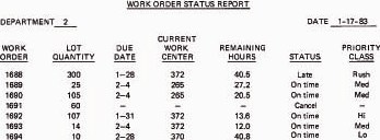
This is similar to the work-in-process function and relies on the same basic data. One of the principal reporting documents in SFC is the Work Order Status Report. As its name suggests, it provides information on the status of the orders in the shop.
This report should be updated several times per week, depending on the nature of the product and the processes in the shop. It might be sufficient to display the report on a CRT rather than in hard-copy form. However, an exception report should be printed periodically in document form. This would indicate the orders that were behind schedule as well as other noteworthy exceptions that happened during the period (e.g., significant machine breakdowns).
The accuracy and currentness of the work order status report are dependent on the correctness and timeliness of the basic data collected in the shop. These data deal with shop order transactions such as job completions, material movement, time turned in against an order, and so on. The method of collecting these data is critical to the success and value of the shop floor control system. The design of this factory data collection (FDC) system can take on various forms and we consider these systems in Sections 16.5 and 16.6.
Production output data for capacity control
Capacity planning is the function of a computer-integrated production management system which determines the labor and equipment resources that will be required to accomplish the master production schedule. It is a planning function. On the other hand, capacity control is concerned with making adjustments in labor and equipment usage to meet the production schedule. To make these adjustments effectively, the capacity control function must have up-to-date information on production rates and order status from the factory data collection system.
16.3 The Shop Floor Control System
The shop floor control system should be designed to accomplish the four functions efficiently and effectively. There are various ways in which the SFC system can be configured, ranging in degrees of computer involvement. At the current level of development in manufacturing technology, none of the shop floor control systems exclude human participation. In other words, SFC systems are not control systems in the sense of automatic feedback control or computer process control.1 Even the most computerized and modern shop floor control systems today require human beings as a vital link in the control loop. The purpose of the computer system in SFC is to generate information by which the human beings can make good decisions on effective factory management and implementation of the master schedule.
1 We consider computer process control in Chapter 18.
The organization of a computerized shop floor control system is illustrated in Figure 16.1. The diagram differentiates between those portions of SFC which are computer driven and those which require human participation. The computer generates various documents which are utilized by people to control production in the factory.
The shop floor control system consists of three steps. These steps are manifested as three computer software modules which are linked together in the SFC system. The three steps or modules are:
1. Order release
2. Order scheduling
3. Order progress
We describe these shop floor control steps in the following subsections.
Order release
The purpose of the order release module is to provide the necessary documentation that accompanies an order as it is processed through the shop. These documents are referred to collectively as the shop packet and their release to the factory constitutes the release of the order. The shop packet for an order consists of:
1. Route sheet–listing the operation sequence and tools needed
2. Material requisitions–to draw the necessary raw materials (or components for assemblies) from stock
3. Job cards–enough job cards to report the labor for each operation on the route sheet
4. Move tickets–to move the parts between work centers
5. Parts list–for assembly jobs
Figure 16.1 Flow of information in shop floor control.

The shop packet moves with the job through the sequence of processing or assembly operations. It comprises the documentation necessary to complete the job and to monitor the status of the job in the shop.
There are two inputs to the order release module. First, the basic information, which indicates that this module should release a particular order, is provided by MRP, capacity planning, and other elements of the computer-integrated production management system. (These elements are shown in Figure 14.2, but not in Figure 16.1.) The second input is the engineering and manufacturing data base, which contains the standard routing file and product structure file. The standard routing file contains the sequence of operations and work centers needed to process the order. This is used to prepare the route sheet in the shop packet. The product structure file contains the bill of materials for material requisitions and parts lists.
Order scheduling
The purpose of order scheduling is to make assignments of the orders to the various machines in the factory. Inputs to this module consist of the order release and priority control. Each job order has a certain priority determined by its due data and other factors. It is the function of priority control to schedule the orders for production according to their priorities. Section 16.4 examines several methods of assigning priorities for production scheduling.
The basic document prepared by the order scheduling module is the dispatch list. It reports the jobs that should be done at each work center and certain details about the routing of the part. One possible format of this dispatch list is shown in Figure 16.2. The dispatch list is generated each day or each shift. In an effective shop floor control system, this document represents to the foreman or production supervisor the best way for accomplishing the master schedule. Certain events may occur, such as a machine breakdown or poor raw materials, which prevent the supervisor from following the dispatch list completely. These exceptions will be reported, and, through subsequent adjustments in priority control, an attempt will be made to put the order back on schedule.
Order progress
The order scheduling module satisfies the first function of shop floor control: priority control and assignment of work orders. The purpose of the order progress module is to accomplish the remaining three functions of SFC: to provide data relative to work-in-process, shop order status, and capacity control. The order progress
Figure 16.2 Dispatch list.

Figure 16.3 Work order status report.
module is designed to accept data collected from the shop floor and to generate reports that can be used to assist production management.
The various documents contained in the shop packet provide the means to identify the job. When a machine operator completes a particular process specified in the route sheet, relevant data to indicate the completion are entered into the order progress module. The data would include such items as piece count, scrap-page (if any), operator identification number, operation number, work centers, and time of completion. The order progress module maintains a file of the transactions reported on each of the uncompleted jobs. This file is called the open order file, and it contains the latest status of each job order in the factory. The types of reports that can be generated from the open order file include the following:
1. Work order status reports. These are detailed reports that show the progress of each job through the shop. One possible format for the work order status report is illustrated in Figure 16.3.
2. Exception reports. These are designed to pinpoint deviations from the production schedule, overdue jobs, inconsistent piece counts (e.g., an increase in the number of pieces in the order), and other exception information.
These reports can be generated daily to achieve better control over jobs in the plant. Depending on the design of the shop floor control system, the information in the open order file might also be obtained on an inquiry basis.
16.4 Operation Scheduling
An overview of the scheduling problem
The master production schedule gives the timetable for end-product deliveries. This is translated into material and component requirements by using MRP, and checked against plant production capacity by means of capacity planning. The next link in this planning chain is operation scheduling, which is performed by the order scheduling module in shop floor control.
Operation scheduling is concerned with the problem of assigning specific jobs to specific work centers on a weekly, daily, or hourly basis. The end products specified in the master schedule consist of components, each of which is manufactured by a sequence of processing operations. Operation scheduling involves the assignment of start dates and completion dates to the batches of individual components and the designation of work centers on which the work is to be performed. The scheduling problem is complicated by the fact that there may be hundreds or thousands of individual jobs competing for time on a limited number of work centers. These complications are compounded by unforeseen interruptions and delays such as machine breakdowns, changes in job priority, work absenteeism, and strikes.
The objectives of an operation scheduling system are to assign jobs to work centers so as to:
1. Meet the required delivery dates for completion of all work on the jobs.
2. Minimize in-process inventory. This is accomplished by minimizing the aggregate manufacturing lead time.
3. Maximize utilization of machines and labor resources.
There are a variety of scheduling methods used in production. Different methods are appropriate, depending on whether the factory is engaged in job shop operations, batch production, or mass production. To describe the operation scheduling problem, let us consider the typical job shop or batch production situation. Jobs are to be processed through the appropriate sequence of work centers. A job is defined as a single part or batch of parts. A job could also consist of groups of components to be assembled. Operation scheduling can be described as consisting of the following two steps:
1. Machine loading
2. Job sequencing
To process the jobs through the factory, the jobs must be assigned to work centers. Since the total number of jobs exceeds the number of work centers, each work center will have a queue of jobs waiting to be processed. Allocating the jobs to the work centers is referred to as machine loading. Ten jobs may be the loading for a particular work center. The unanswered question is: In what sequence will the 10 jobs be processed? Answering this question is the problem in job sequencing.
Job sequencing involves determining the order in which to process the jobs through a given work center. To accomplish this, priorities are established among the jobs in the queue. Then the jobs are processed in the order of their relative priorities. When a job is completed at one work center, it enters the queue at the next work center in its process routing. That is, it becomes part of the machine loading for the next work center, and the priority rule determines its sequence of processing among those jobs.
Priority rules for job sequencing
A priority rule in operation scheduling is a guide for determining the sequence in which jobs will be processed through a given work center. Some of the priority rules used in industry are the following:
Highest priority is given to jobs with the “earliest due date.”
Highest priority goes to the job with the “shortest processing time.”
Jobs are processed on a “first-come-first-serve” basis.
Highest priority is given to the job with the “least slack” in its schedule,
where slack is defined as follows:
slack = (time remaining until due date) - (process time remaining) (16.1)
Highest priority is given to the job with the lowest “critical ratio” where the critical ratio is defined as follows:
![]()
The “red tag” method, where rush jobs are identified with a red ticket by the expediter.
An example will help to illustrate how these priority rules are used to determine the sequence in which jobs would be processed.
Example 16.1
Suppose that we are presently at day 15 on the production scheduling calendar for the G ' Z Machine Company and that there are three jobs (shop orders A, B, and C) in the queue for a particular work center. The jobs arrived at the work center in the order A, then B, then C. The following table gives the parameters of the scheduling problem for each job:

Using the “earliest due date” we would schedule the jobs in the order C-A-B. With the “shortest processing time” priority rule, the jobs would be schedule A-C-B. If jobs were scheduled first-come-first-serve, the sequence would be A-B-C.
Using the “least slack” rule, we would determine the slack for each job according to Eq. (16.1). For job A, the slack is (25 - 15) - 5 = 5 days. For job B, the slack is (34 - 15) - 16 = 3 days. And for job C, slack = (24 - 15) - 7 = 2 days. The jobs would be processed in the order C-B-A.
Finally, using the “critical ratio” to establish order priority, Eq. (16.2) would be used for each job. For job A, the critical ratio = (25 - 15)/5 = 2.0 For job B, the critical ratio = (34 - 15)/16 = 1.19. For job C the critical ratio = (24 - 15)/7 = 1.29. The processing sequence would be B—C–A.
The results are summarized in the following table
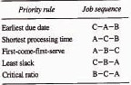
The reader will note that, for the data of this example, five different priority rules have yielded five different job sequences.
The question of which among the solutions is the best depends on one’s criteria for defining what is best. The shortest processing time rule will usually result in the lowest average manufacturing lead time and therefore the lowest in-process inventory. However, this may result in customers whose jobs have long processing times to be disappointed. First-come-first-serve seems like the fairest criteria, but it denies the opportunity to deal with differences in due dates among customers and genuine rush jobs. The earliest due date, least slack, and critical ratio rules address this issue of relative urgency among jobs. Then there is the “red tag” priority rule (not considered in Example 16.1), the method used by expediters to indicate which jobs should be processed on a “rush” basis. The trouble with the red tag method is that shops often end up with more jobs red tagged than not.
Let us evaluate the five priority rules used in Example 16.1 in terms of manufacturing lead time and job lateness.
Example 16.2
For example 16.1, assume that the work center to which the data apply is the final work center in the routing for each of the three jobs. Accordingly, the remaining process time refers to that work center. The problem is to determine the average manufacturing lead time for the three jobs and the aggregate job lateness for the three jobs.
The manufacturing lead time for each job is the remaining process time plus time spent in the queue waiting to be processed at the work center. The average manufacturing lead time is the average for the three jobs.
Job lateness for each job is defined as the number of days the job is completed after the due date. If it is completed before the due date, it is not late. Therefore, its lateness is zero. The aggregrate lateness is the sum of the lateness times for the individual jobs.
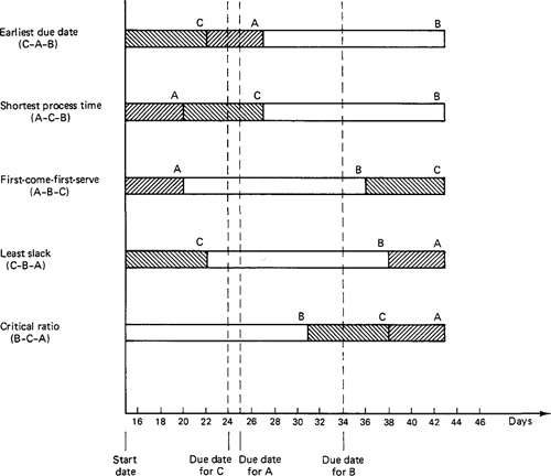
Results of the processing through the last work center are displayed on the time chart of Figure 16.4 for each of the five priority rules considered in Example 16.1.
Using the earliest due date rule to illustrate the arithmetic, the lead time for job C is its processing time of 7 days. The lead time of job A is its waiting time plus processing time = 7 + 5 = 12 days. The lead time of job B is 7 + 5 + 16 = 28 days. The average is (7 + 12 + 28)/3 = 15% days.
Job lateness for job C under the earliest due date rule is zero since it is completed before its due date. Job A is 2 days late and job B is completed 9 days behind schedule. The aggregate job lateness is 11 days.
Figure 16.4 Results of Example 16.2 for five priority rules.
The results for all five rules are summarized in the following table:

The relatively simple earliest due date and shortest process time rules seem to perform best for the data of this example. Any of the common priority rules can be programmed into the order scheduling module of a shop floor control system. As Example 16.2 illustrates, the firm must be careful to select a priority rule or combination of rules that accomplish its desired scheduling objectives.
16.5 The Factory Data Collection System
The purpose of the factory data collection (FDC) system in shop floor control is to provide basic data for monitoring order progress. In a computerized SFC system these data are submitted to the order progress module for analysis and generation of work order status reports and exception reports. The types of SFC data that would be collected by the FDC system include:
Piece counts
Count on scrapped parts or parts needing rework
Completion of operations in the routing sequence
Machine breakdowns
Labor time turned in against a job
These parameters of factory activity represent the basic data from which status information on shop orders can be determined.
Another purpose for which a factory data collection system may be used is time and attendance reporting for accounting and payroll departments. Many FDC systems include terminals for employees to clock in and clock out at the beginning and end of the shift. These types of records are often incorporated into the shop floor control system.
Kasarda [14] lists five methods that have been used to collect data from the shop floor:
2. Employee time sheet
3. Operation tear strips or punched cards included with shop packet
4. Centralized shop floor terminals
5. Individual work center terminals
All of these methods require the coorperation of the shop workers in recording the data on a paper document or entering the data at a computer terminal. Job travelers and time sheets are the most manual and clerical approaches, while individual work center terminals represent the least manual (and highest initial investment) approach. Our interest is more with the computerized FDC systems (central terminals and work center terminals), but we will describe the manual approaches first.
Job traveler
The job traveler is basically a log sheet that is included with the shop packet moving with the job through the various work centers specified on the route sheet. Each employee who works on the job is required to record the time spent, piece counts, and other data onto the log sheet. When the job is completed, the sheet contains the complete history for that shop order. It can be reviewed, analyzed, and summarized by production control, accounting, and others.
From the standpoint of shop floor control, there are several important disadvantages with this method and little that can be said in its favor. It is perhaps the easiest method to implement and does not require use of a computer. Among its disadvantages, one is the problem that no data are collected on the order until the shop has completed all processing. Therefore, it is not possible to determine the work status of the order during process, except by physically locating the order in the factory and visually determining its status. This hardly satisfies the functions of shop floor control. Another problem is the accuracy and reliability of the data recorded on the log sheet. It is not possible to detect errors in the log sheet as they are being recorded. Because of its significant disadvantages, use of the job traveler does not lend itself to a computerized shop floor control system.
Employee time sheet
A second method of shop data collection is the employee time sheet. A time sheet is prepared by each worker, detailing information about the order. The employee must copy data (e.g., order number, operation number, etc.) onto the time sheet from the shop packet that accompanies the job. The time spent on the order, quantities produced, and similar data must also be recorded.
One big advantage of the employee time sheet method over the job traveler is that the data are submitted in a much more timely manner. Time sheets can be turned in each shift, thus allowing the status of an order to be determined on a more current basis. This does not happen automatically. It requires a clerical employee to summarize the data and an alert foreman to track down any problems or discrepanices which are indicated by the time sheets. The clerical procedure involves a time lag which delays the reporting on order status.
This delay is one of the disadvantages of the time sheet method. The order status report may not be prepared until several days after the work is reported. This is probably too late for factory managment to react to a problem effectively. A second disadvantage is that the time sheet method still relies on the employee to transcribe the data. Clerical errors may result from this manual procedure.
Operation tear strips
This represents an attempt to reduce the amount of clerical detail work involved with the job traveler and time sheet methods. Instead, when the shop packet is prepared at the time of order release, a set of preprinted tear strips or prepunched cards are also generated. These tear strips or cards follow the job through the factory together with the shop packet. When a worker finishes a particular operation on the job, one of the tear strips or cards is turned in. The employee must record only a minimum of data, such as piece count completed, since all the other information has been preprinted or prepunched.
The job tickets can be submitted daily or at the completion of an operation on the job which may occur during the shift. With the assistance of a clerical employee working at a computer terminal, job status data can be turned in to the SFC order progress module in a fairly timely fashion.
The disadvantages of the tear strip (or prepunched job ticket) method are that the tickets may get lost (of course, this could happen to the entire shop packet) or that an insufficient quantity of tickets will be prepared. Also, there is a time delay between when the tickets are turned in and when the clerk reports them into the order progress module.
Centralized shop terminal
To overcome the disadvantages of the previous clerical methods, the use of data entry terminals in the shop has been introduced. This approach ranges from the installation of one central terminal to the use of individual workstation terminals. We discuss the individual workstation terminals in the next subsection.
The centralized terminal approach may consist of a single terminal located near the center of the plant. If the plant is large, this may require some employees to walk great distances to enter the order data. A variation of the central terminal approach is to have a limited number of satellite terminals strategically located at convenient and accessible points throughtout the shop.
The use of central terminals requires that human operators enter the data manually. Workpiece counts, operation number, machine downtime, and product quality data are examples of data that can be entered by means of human operators located in the shop. In discrete-parts manufacturing, manual entry stations constitute a common form of factory data collection system in use today. The terminals range in complexity from simple pushbutton devices to sophisticated typewriter keyboard units with built-in microprocessor and data storage capability. Factory workers must be trained to key in the proper data, including operator identification number, the type of data being reported, and the data themselves in correct format.
Shop floor data entered from manual entry stations can be communicated directly to the computer. This is sometimes referred to as an “on-line” system. The alternative is to use an “off-line” configuration, in which the data are collected and stored in a data storage device for subsequent processing by the computer. An example of a system that can operate in either mode is the IBM 3630 Plant Communication System [13], which consists of various types of data-entry terminals, output devices, communication links, and a controller. The data-entry stations capture information from the factory, such as production piece counts, inventory counts, material and job status data, quality inspection data, job times (for costing purposes), and tool usage data. Factory management defines the type of information to be collected by the system. The time entry stations are located at entrance and exit doors and serve the function of time clocks to punch in and out. The controller unit collects and stores the data from the various entry stations. The shop records can be stored on diskettes for processing by the plant computer to generate the desired reports. Figures 16.5, 16.6, and 16.7 show a variety of data-entry terminals available on the IBM 3630 system.
The disadvantage of the centralized FDC system is the inconvenience to the operator, who may have to waste time walking back and forth to the one central
Figure 16.5 IBM 3647 Time and Attendance Terminal with magnetic card reader port. (Courtesy of IBM Corp.)

Figure 16.6 IBM 3641 Reporting Terminal used by workers to input work order data in the factory. (Courtesy of IBM Corp.)

Figure 16.7 IBM 3643 Keyboard Display, an interactive terminal for plant use. (Courtesy of IBM Corp.)

input terminal. At the end of the shift there will probably be other workers waiting to use the same terminal.
Another potential disadvantage arises in the case of the off-line entry configuration. In this system, the data entered may be stored until the end of the shift and then batch processed on the computer. This results in a delay on the reporting of order status which may be no less than in the tear strip method of factory data collection. The company may have invested thousands of dollars in a central terminal installation which provides results that are little better than the manual method.
Individual work center terminals
The ultimate FDC system for convenience and responsiveness is the individual work center entry terminal. The convenience to the operator results from the fact that the terminal is located in the immediate work area, perhaps attached to the machine tool or other processing equipment. The system should be more responsive than other methods because the operator can report status on the order more frequently; hence status reports are more current.
It is possible with the work center terminal to customize the front panel and other features of the entry device to facilitate the types of inputs which are likely to be made at that workstation. The order progress module can be programmed to properly interpret abbreviated inputs when entered at a particular work center. All of this results in simpler and faster data entry for the operator.
Cost is an important factor in the workstation terminal FDC systems. To be economically justified, the cost of each terminal must be low enough to make the installation worthwhile. Several hundred dollars is probably the upper limit on price per terminal installation.
The next logical step beyond the individual workstation terminal is to establish a direct connection between the workstation and the computer, uninterrupted by the necessity for a human operator to enter the data manually on a data entry device. This is the subject of computer process monitoring which we discuss in Section 16.6. One final manual input method might be mentioned before discussing this computer-automated technique.
Voice data input
In Section 8.9 we discussed voice numerical control, a method for programming numerically controlled machine tools. Another use of voice–computer communication is data input for manufacturing information systems. This technology is sometimes referred to as automatic speech recognition and it represents an attempt to simplify the human–machine interface. Under the proper circumstances, voice entry of information to the computer represents the easiest and quickest method of input. Examples of applications in manufacturing include quality inspection, inventory control, and part identification. There is potential for applying these systems in shop floor control data collection.
The characteristics that make a good industrial application of an automatic speech recognition system are described in Ref. [10]. First, there must be an existing computerized reporting system. Second, the data entry steps must be repetitive. Third, use of voice input requires a limited number of operators using the system. Most voice systems are speaker dependent, which means that the speech recognition processor recognizes only the unique voice patterns of the individuals who use the system. Fourth, a reasonable vocabulary is required to enter the data. This usually means a limitation of several dozen words. Fifth, it is desirable to capture the production data at the source.
Example 16.3
An example of a factory data collection system and factory management system is reported in Ref. [6]. The system is installed at Hughes Aircraft Company’s Microelectronics Technology Division in Fullerton, California, and is called FAMIS (FActory Management Information System). It was developed as a turnkey hardware and software system by Digital Datacom, Inc. The system consists of the central computer, disk memory and file storage, video display terminals, printers, and several card readers. A job traveler FDC system is used, where the traveler tickets are prepared on the printers as needed. These tickets contain all the data needed to report on order status. The job tickets are mark-sensitive tab cards, which allows work entries to be made with an ordinary number 2 pencil. These penciled entries consist of checks in boxes printed on the tab card. The job card is then inserted into the card reader to enter data. FAMIS is used to generate a variety of management reports on production and quality performance.
16.6 Computer Process Monitoring
All the factory data collection systems described in the preceding section required some form of human participation. Computer process monitoring (also sometimes called computer production monitoring) is a data collection system in which the computer is connected directly to the workstation and associated equipment for the purpose of observing the operation. The monitoring function has no direct effect on the mode of operation except that the data provided by monitoring may result in improved supervision of the process. The industrial process is not regulated by commands from the computer. Any use that is made of the computer to improve process performance is indirect, with human operators acting on information from the computer to make changes in the plant operations. The flow of data between the process and the computer is in one direction only—from process to computer.
The components used to build a computer process monitoring system include transducers and sensors, analog-to-digital converters (ADC), multiplexers, realtime clocks, and other electronic devices. Many of these components are described in Chapter 17. These components are assembled into various configurations for process monitoring. We discuss three such configurations:
1. Data logging systems
2. Data acquisition systems
3. Multilevel scanning
A particular computer process monitoring system is highly custom designed and may consist of a combination of these possible configurations. For example, a data acquisition system may include multilevel scanning.
Data logging systems
A data logger (DL) is a device that automatically collects and stores data for offline analysis. Strictly speaking, the data could be analyzed by a person without the aid of computer. Our interest here is in data logging systems that operate in conjunction with computers. Data loggers can be classified into three types [4]:
1. Analog input/analog output
2. Analog input/analog and digital output
3. Analog and digital input/analog and digital output
Type 1 can be a simple one-channel strip chart recording potentiometer for tracking temperature values using a thermocouple as the sensing device. Types 2 and 3 are more sophisticated instruments which have multiple input channels and make use of multiplexers and ADCs to collect process or experimental test data from several sources. The DL can be interfaced with tape punches, magnetic tape units, teletypes and printers, plotters, and so on. They can also be interfaced with the computer for periodic transfer of data.
A programmable data logger (PDL) is a device that incorporates a microprocessor as part of the system. The microprocessor serves as a controller to the data logger and can be programmed by means of a keyboard. The programmable data logger can easily accommodate changes in rate or sequence of scanning the inputs. The PDL can also be programmed to perform such functions as data scaling, limit checking (making certain the input variables conform to prespecified upper and lower bounds), sounding alarms, and formatting the data to be in a compatible and desirable format with the interface devices.
Data acquisition systems
The term data acquisition system (DAS) normally implies a system that collects data for direct communication to a central computer. It is therefore an on-line system, whereas the data logger is an off-line system. However, the distinction between the DL and the DAS has become somewhat blurred as data loggers have become directly connected to computers.
Data acquisition systems gather data from the various production operations for processing by the central computer. The basic data can be analog or digital data which are collected automatically (transducers, ADC, multiplexers, etc.). It is a factory-wide system, as compared with data loggers, which are often used locally within the plant. The number of input channels in the DAS is therefore typically greater than in the DL system. For the data logger the number of input channels might range between 1 and 100, while the data acquisition system might have as many as 1000 channels or more. The rate of data entry into the DL system might
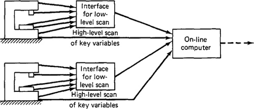
Figure 16.8 Multilevel scanning in computer process monitoring.
be 10 readings per second for multiple-channel applications. By contrast, the DAS would have to be capable of a data sampling rate of up to 1000 per second. Because of these differences, the data acquisition system would be typically more expensive than the data logger.
Multilevel scanning
In the data acquisition system, it is possible for the total number of monitored variables to become quite large. Although it is technically feasible for all these variables to be monitored through multiplexing, some of the signals would not be needed under normal operating conditions. In such a situation it is convenient to utilize a multilevel scan configuration, as illustrated schematically in Figure 16.8. With multilevel scanning, there would be two (or more) process scanning levels, a high-level scan and a low-level scan. When the process is running normally, only the key variables and status data would be monitored. This is the high-level scan. When abnormal operation is indicated by the incoming data, the computer switches to the low-level scan, which involves a more complete data logging and analysis to ascertain the source of the malfunction. The low-level scan would sample all the process data or perform an intensive sampling for a certain portion of the process that might be operating out of tolerance.
References
[1] AMERICAN PRODUCTION and INVENTORY CONTROL SOCIETY, Shop Floor Controls, 1973.
[2] BAILEY, S. J., “Data Acquisition Systems Mature into Control Loop Decision Makers,” Control Engineering, February, 1982, pp. 66–70.
[3] BOEING COMPUTER SERVICES COMPANY, PMS (Production Management System), The Boeing Company, 1979.
[4] BROWN, J., “Choosing between a Data Logger (DL) and Data Acquisition System (DAS),” Instruments and Control Systems, September, 1976, pp. 33–38.
[5] CHASE, R. B., and AQUILANO, N. J., Production and Operations Management, 3rd ed., Richard D. Irwin, Inc., Homewood, Ill., 1981, Chapter 14.
[6] “FAMS SPELLS SAVINGS,” Assembly Engineering, October 1981, pp. 42–44.
[7] GREEN, A. M., “Shop Floor Data Closes the Loop in Factory Management,” Iron Age, September 28, 1981, pp. 75–79.
[8] GROOVER, M. P., Automation, Production Systems and Computer-Aided Manufacturing, Prentice-Hall, Inc., Englewood Cliffs, N.J., 1980, Chapters 12, 17.
[9] HALEVI, G., The Role of Computers in Manufacturing Processes, John Wiley ' Sons, Inc., New York, 1980, Chapter 9.
[10] HUBER, R. F., “Tell It to Your Machines,” Production, June, 1980.
[11] INTERNATIONAL BUSINESS MACHINES CORPORATION, Production Information and Control System, Publication GE20-0280-2.
[12] INTERNATIONAL BUSINESS MACHINES CORPORATION, Communications Oriented Production Information and Control System, Vol. I, Publication G320-1974.
[13] INTERNATIONAL BUSINESS MACHINES CORPORATION, IBM 3630 Plant Communication System, System Description, Publication GA24-3652-2, Endicott, N.Y., 1979.
[14] KASARDA, J. B., “Shop Floor Control Must Be Able to Provide Real-Time Status and Control,” Industrial Engineering, November, 1980, pp. 74–78, 96.
[15] MAY, N., “Shop Floor Controls—Principles and Use,” Proceedings, Twenty-fourth Annual International Conference, American Production and Inventory Control Society, Boston, October, 1981, pp. 170–174.
[16] MONKS, J. G., Operations Management: Theory and Problems, McGraw-Hill Book Company, New York, 1977, Chapter 9.
[17] RAFFISH, N., “Let’s Help Shop Floor Control,” Production and Inventory Management Review and APICs News, American Production and Inventory Control Society, July, 1981, pp. 17–19.
[18] RAFFISH, N., “The Engineer’s Impact on Shop Floor Control,” Manufacturing Engineering, February, 1982, pp. 59–61.
[19] WIGHT, OLIVER W., Production and Inventory Management in the Computer Age, Cahners Books, Boston, 1974, Chapter 8.
Problems
16.1. Four jobs are to be scheduled through a certain work center. The following table gives data regarding the due date (values given are in terms of the production calendar day) and remaining process time.

In the shop calendar, the current date is day 10.
(a) Use the “earliest due date” priority rule to set the production sequence for these jobs.
(b) Use the “shortest processing time” rule to establish the sequence.
(c) Use the “least slack” rule to sequence the jobs.
(d) Use the “critical ratio” to sequence the jobs.
16.2. For the solutions of Problem 16.1, evaluate the results using the criteria of average manufacturing lead time and aggregate job lateness. It is suggested that the reader plot the results on a time chart similar to Figure 16.4.
16.3. Three jobs are currently waiting in the queue to be processed through a certain milling machine. Following the milling operation, each of the jobs must be processed through a surface grinder. There is no queue of work at the grinder nor is it anticipated that there will be between now and when these jobs are processed. The processing times at the two machines for each of the three jobs are given in the following table, together with the due dates.

Assume that the present date is day zero.
(a) Use the earliest-due-date rule to schedule the jobs through the milling machine.
(b) On a piece of graph paper, devise a method of plotting the progress of the three jobs as they are each processed through the milling machine and the grinding machine.
(c) Determine the average manufacturing lead time and the aggregate job lateness for this schedule.
16.4. Solve Problem 16.3 except use the shortest-processing-time rule instead of the earliest-due-date rule.
16.5. Solve Problem 16.3 except use the least-slack rule instead of the earliest-due-date rule.
16.6. Solve Problem 16.3 except use the critical ratio to schedule the jobs instead of the earliest-due-date rule.