Chapter 17
Computer-Process Interfacing
17.1 Introduction
In this part of the book we consider how computers are used to control manufacturing processes. In this first chapter, the problem of interfacing the computer with the process is examined. In Chapter 18 we survey the various types of computer process control systems, such as direct digital control (DDC) and supervisory computer control. Chapter 19 is concerned with the technology of quality inspection and quality control by means of computers. Finally, Chapter 20 presents a good example of computer process control in manufacturing by examining computer-integrated manufacturing systems.
To be useful,the computer must be capable of communicating with its environment.In a data processing system, this communication is accomplished by the various input/output devices discussed in Chapter 2, such as card readers, printers, and CRT consoles. In computer-aided manufacturing, the environment of the computer includes not only these devices but also includes one or more manufacturing processes. Functioning as a process control system, the computer must be capable of sensing the important process variables from the operation and providing the necessary responses to maintain effective control over the process. In the following sections we examine some of the important components of a computer process control system.
17.2 Manufacturing Process Data
Let us begin by considering the nature of the data that must be communicated between the manufacturing process and the computer. These data can be classified into three categories:
1.Continuous analog signals
2.Discrete binary data
3.Pulse data
Continuous analog data can be represented by a variable that assumes a continuum of values over time. During the manufacturing process cycle, it remains uninterrupted, and the values it can assume are restricted to a finite range. Examples of analog variables include temperature, pressure, liquid flow rate, and velocity. Each of these phenomena are continuous functions over time and are capable of taking on an infinite number of values in a certain range. The number of values permitted is a function of the ability of measuring instruments to distinguish between different signal levels.
Discrete binary data can take on either of two possible values, such as on and off, or open and closed. Switches, motors, valves, and lights are all devices whose status at any time may be a binary function. Binary-valued process variables can represent many situations, such as:
The state of a machine tool (automatic or controlled cycle, operational or down, workpart in place or station empty, etc.).
The state of special sensing switches which permit the process to continue. For example, some industrial robot installations include several switch devices under a floor mat which close under the weight of an intruding worker. The closed state of the switch is interpreted as a hazard condition under which robot motion is stopped and alarm devices are activated.
Binary data are represented in electronic digital systems as typically one of two voltage levels whose values depend on the specific devices that make up the system. Typical voltage levels are 0 and +5V.
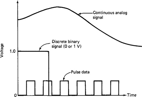
Pulse data consist of a train of pulsed electrical signals from devices called pulse generators. The pulse train can be used to drive devices such as stepping motors. The magnitude of each pulse is fixed; the magnitude of the pulse train is the number of pulses it contains. Since the number of pulses in a series can be counted over a period of time, that number can be represented as digital data. Conversely, digital data can be used to produce a pulse train of a given magnitude. The three general types of manufacturing process data are illustrated in Figure 17.1
Figure 17.1 Three types of manufacturing process data.
17.3 System Interpretation of Process Data
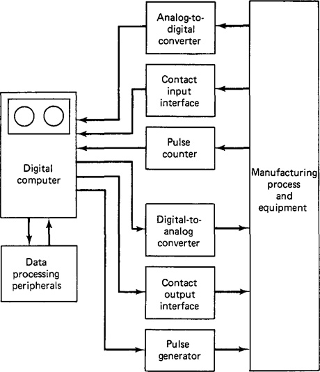
The three categories of manufacturing process data must be capable of interacting with the computer. For monitoring the process, input data must be entered into the computer. For controlling the process, output data must be generated by the computer and converted into signals understandable by the manufacturing process. There are six categories of computer-process interface representing the inputs and outputs for the three types of process data. These categories are:
1. Analog to digital
2. Contact input
3. Pulse counters
4. Digital to analog
5. Contact output
6. Pulse generators
The general configuration of the computer process interface is illustrated in Figure 17.2.
Analog-to-digital interfacing involves transforming real-valued signals into digital representations of their magnitude. A number of different steps must be accomplished to effect this conversion process. These steps involve the following hardware:
1. Transducers, which convert a measurable process characteristic (flow rate, temperature, process, etc.) into electrical voltage levels corresponding in magnitude to the state of the characteristic of the process
Figure 17.2 Computer-process interface.
measured. A thermocouple is an example of a device in this category. It converts temperature into a small voltage level.
2. Signal conditioners, which filter random electrical noise and smooth the analog signal emanating from transducing devices.
3. Multiplexers, which connect several process-monitoring devices to the analog-to-digital converter. Each process signal is sampled at periodic intervals and passed on to the converter.
4. Amplifiers scale the incoming signal up or down to the range of the analog-to-digital converter being used.
5. The analog-to-digital converter (ADC) transforms the incoming real-valued process signals into their digital equivalents.
6. The digital computer’s I/O section accepts the digital signals from the ADC. A limit comparator is often connected between the I/O sections and the ADC to prevent out-of-limit signals from distracting the CPU.
The contact input interface is a set of simple contacts that can be opened and closed to indicate the status of limit switches, button positions, and other binary-type data. It serves as the intermediary between discrete process data and the computer, which periodically scans the signal status and compares it with preprogrammed values.
Digital transducers belong to a class of electronic measuring instruments that generate as output a series of electrical pulses of uniform magnitude. A pulse counter is used to convert the pulse trains into a digital representation, which is then applied to the computer’s input channel. The last three devices discussed are concerned with processing data from the computer to the process.
The digital-to-analog converter takes digital data generated by the computer and transforms it into a pseudoanalog signal. The signal is considered pseudoanalog because the computer is only capable of a limited-precision digital word, so that an infinite number of analog signal levels cannot be generated.
Contact output interfaces, like their input counterparts, are sets of contacts that can be opened or closed. The output word of the computer is used to turn on indicator lights, alarms, and even equipment functions such as cutting oil pumps.
Pulse generators are frequently used as output devices which convert digital words from the computer into pulse trains that are used to drive devices such as stepping motors.
17.4 Interface Hardware Devices
Hardware components are required to accomplish the computer—process interface described in the preceding section. In this section we consider some of these hardware devices.
Transducers and sensors
A transducer converts one type of physical quantity into another which can be more conveniently used and evaluated. When transducers are used to measure the value of a physical quantity, they are referred to as sensors. There are two types of transducers: analog and digital.
An analog transducer generates a continuous signal, such as an electrical voltage or current, that can be interpreted as the value of a measured process variable. A calibration between the measured variable and the output signal is required to determine the exact nature of their correspondence. Signals generated by these transducers are classified as low-level (measured in millivolts) and high-level (greater than 1 V).
A digital transducer generates a digital signal in the form of a set of parallel bits or a series of countable pulses. The output of the transducer represents the quantity measured by it. Because of their compatibility with digital computers and the ease with which they can be read when used as stand-alone instruments, digital transducers are finding increased use in industrial applications.
Analog-to-digital converters
An analog-to-digital converter (ADC) is a device that transforms a continuous analog signal into digital form. The process of converting the analog signal into a digital value occurs in three phases:
1. The continuous signal is periodically sampled to form a series of discrete-time analog signals.
2. Each discrete analog value falls within one of a finite number of predefined amplitude levels called quantization levels, which consist of discrete voltages over the range of the device.
3. The amplitude levels are converted into digital form. This phase is sometimes called encoding.
In selecting an analog-to-digital converter for a particular manufacturing process application, consideration must be given to the operating characteristics of the ADC device. Among these characteristics are the following:
Sampling rate. This is the rate at which the analog signal is sampled. The higher this rate, the more closely approximated the signal will be. High sampling rates are also very important for multiplexed systems, in which all signals must be sampled in a short period of time. The upper limit on the sampling rate is imposed by the conversion time of the ADC.
Conversion time for an applied analog signal to be transformed into a digital output.
Resolution of the ADC. Resolution refers to the precision with which an analog signal can be represented in digital form. It is determined by the number of quantization levels, which depend on the number of bits used by the ADC. The number of quantization levels available is given by:
number of quantization levels = 2N(17.1)
where N is the number of bits used by the ADC. The resolution of the device would be the reciprocal of the number of quantization levels. The spacing between adjacent quantization levels would be the full-scale value for the incoming analog signal divided by the number of quantization levels. The incoming analog signal is typically amplified to provide a full scale of 0 to 10 V. The following example will illustrate these concepts of quantization levels, resolution, and spacing between quantization levels.
Example 17.1
A continuous-voltage signal is to be converted to digital form by an ADC. The actual full-scale range of this voltage is zero to 2.0 V, but an amplifier is used to magnify this range to zero to 10 V. A 10-bit analog-to-digital converter will be used. It is desired to determine the number of quantization levels, the resolution, and the spacing between adjacent quantization levels.
According to Eq. (17.1), the number of quantization levels is
210 = 1024 levels
The resolution would be the reciprocal of the number of quantization levels:
resolution = (1024)-1 = 0.00097 = 0.097%
Finally, the spacing between adjacent quantization levels is the full-scale value of 10 V, divided by the number of quantization levels:
![]()
There are a variety of methods used to convert an analog signal into digital form. Two methods that we will describe are:
1. Successive approximation method
2. Integrating ADC method
In the successive approximation method, trial voltages are compared to the incoming analog signal. Special circuitry yields a “1” when the input voltage exceeds the trial voltage, and a “0” when the input voltage is less than the trial voltage. After each successive iteration, the trial voltage is decremented to half of its previous value. For 6-bit precision conversion time is typically 9 (xs for this method.
Example 17.2
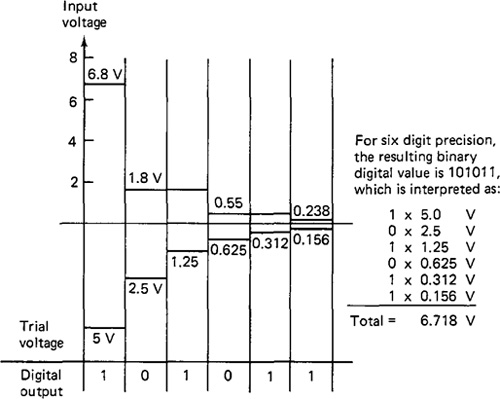
It is desired to use a successive-approximation-type ADC to encode an incoming signal whose full scale value is 10 V. Let us suppose that during the moment of conversion the signal value is 6.8 V. Our ADC has 6-bit precision. The process of converting the signal is illustrated in Figure 17.3.
The first trial voltage is 5.0 V. Comparing the input signal to this value yields a “1” since the input exceeds the trail voltage. Accordingly, the difference of 6.8 V - 5.0 V = 1.8 V is compared with the next trail voltage of 2.5 V (one-half the initital trail voltage). In this comparison, a “0” results because the 1.8 V is less than 2.5 V. This successive approximation procedure is repeated for all 6 bits. The resulting value is 6.718 V. The error between this value and the actual input signal of 6.8 V illustrates the limitation imposed by a 6-bit ADC.
The integrating ADC method is based on converting the applied analog signal into measurable time periods. In the simplest form, the single-slope converter, the input signal is compared to a linearly increasing voltage (a ramp function), and the time required to reach this voltage is measured. This time is proportional to the level of the applied signal. The resolution of this method depends on the frequency
Figure 17.3 Successive-approximation-method analog-to-digital conversion.
of the time-counting pulse train and the slope of the ramp voltage. Highest precision is made possible by high-frequency pulse trains and low ramp slopes. Integrating ADC is slower than successive approximation, with a typical 6-bit resolution conversion taking about 14 JJLS. However, it tends to be more accurate in noisy environments because it is less susceptible to random electrical noise. Random noise tends to be both positive and negative, and therefore its integration tends toward zero.
Digital-to-analog converters
The digital-to-analog converter (DAC) performs the reverse function of the ADC. It receives data from the computer and generates analog voltages which can be used to drive analog devices such as data recorders and plotters. In a sense, the DAC is the computer’s communication link back to the process it is measuring.
Digital-to-analog conversion takes place in two steps. First, the digital data are converted into their analog equivalent. This is called decoding. It is accomplished by a binary register in the DAC which controls the output of a reference voltage source depending on the number of bits contained in the register. Each bit controls one-half the voltage of the preceding bit. The voltage produced is determined by
V0 = VreftO.SBj + 0.2552 + 0.12553 + ... + (2n)-1BH](17.2)
were V0 = output of the decoding operation
Vref = reference voltage source which equals full scale output.
B1, B2, ... , Bn = status (zero or 1) of successive bits in the register
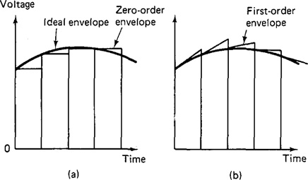
In the second step of the conversion, a data-holding device converts the sampled data from the binary register to an approximation of the continuous analog signal. It attempts to approximate the ideal envelope formed by the sampled data. The order of the extrapolation carried out to approximate the envelope characterizes the DAC device. A zero-order data hold approximates the continuous function with a series of step voltages derived from the binary register. In first-order approximation, the voltage changes with constant slope between sampling instants, sometimes producing a more accurate envelope. Operation of the zero-order and first-order holds is illustrated in Figure 17.4.
With relation to the output of the decoding operation V0 as defined by Eq. (17.2), we can mathematically express the result of the data-holding operation for the zero-order approximation as follows:
V(t) = V0 (17.3)
where V(t ) would be maintained at a constant voltage level during the sampling period.
For the first-order hold, the voltage output during the sampling interval can be expressed as:
V(t) = V0+ at (17.4)
![]()
Figure 17.4 Data-hold function: (a) zero-order; (b) first-order hold.
a = rate of change of V(t)
t = time interval between sampling instants
V0(–t) = value of V0 at the preceding sampling instant
Operation of a DAC device will be illustrated by means of the following two examples.
Example 17.3
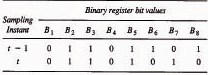
A digital-to-analog converter uses a reference voltage source of 10 V and uses a binary register with six-digit precision. In two successive sampling instants 0.5 s apart, the data contained in the binary register are as follows:
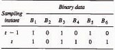
The DAC uses a zero-order hold to maintain the voltage output between sampling instants. Determine the voltage output during the sampling interval following instant t.
The result of the decoding operation can be determined from Eq. (17.2) for the values of B 1, B2, ..., Bn. For interval t,
V0 =10[0.5(1) + 0.25(0) + 0.125(1) + 0.0625(1) + 0.03125(0) + 0.015625(1)] = 7.03125 V
The operation of the data-hold device, as defined by Eq. (17.3) would be to maintain this voltage level for the duration of the sampling interval.
Example 17.4
Using the same data as given in Example 17.3, determine the voltage level during the sampling interval for a DAC with a first-order hold.
To solve this problem, the voltage output of the decoding operation must be determined for instant t – 1 as well as instant t. At instant t – 1,
V0 = 10[0.5(1) + 0.25(0) + 0.125(1) + 0.0625(0) + 0.03125(1) + 0.015625(0)] = 6.5625 V
At instant t, the value of V0 was calculated in Example 17.3 to be 7.03125 V.
To determine the output of the first-order data-hold device, Eqs. (17.4) and (17.5) are used. The rate of change must first be computed according to Eq. (17.5):
Next, the voltage output during the time interval following instant t is given by Eq. (17.4):
V(t) = 7.03125 + 0.9375f
At the beginning of the interval the voltage would be 7.03125 V. The voltage would steadily increase until its value at the end of the sampling interval would be 7.03125 + 0.9375(0.5) = 7.5V.
Multiplexers
The multiplexer is a switching device connected in series with each input channel from the process. It is used to time-share the analog-to-digital converter (and associated amplifiers) among the incoming signals. The alternative to the use of the multiplexer would be to have a separate ADC for each transducer. This would be expensive for a large installation with many inputs to the computer. Since the process variables need only be sampled periodically anyway, the multiplexer provides a very cost effective method of satisfying system design requirements.
17.5 Digital Input/Output Processing
The computer program brings together the many aspects that make up computer monitoring and control of industrial processes. The control software makes use of the computer’s I/O channels. The ADC devices read data from the transducers and the DACs control the servomechanisms that effect change in the processing system. Programming for computer control differs from the conventional programming in that it must deal with:
Timer-initiated events such as the regular sampling of data from process monitoring devices
Process-initiated interrupts which cause special routines to be executed to alleviate an abnormal condition
Passing commands to real-time processes
System- and program-initiated events related to the computer system, such as the transfer of data between computers
Operator-initiated events, such as status or data printout requests, startup or halt instructions, or changes in existing programs
The following sections describe how the process control computer deals with these events. An important feature in control programming is the interrupt system.
Interrupt system
Computers which are programmed to perform control functions are equipped with an interrupt logic system. The purpose of this system is to permit program control to be switched between different programs and subroutines in response to requests by devices in the operating environment. Interrupts can, for example, signal that a work station is empty, and cause a new part to be moved into place.
External interrupts are initiated by events external to the computer, such as the operator or process devices. Internal interrupts are generated in response to an internal timer or other system program events.
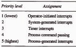
Interrupts are arranged in priority structures that allow critical functions to be carried out before routine tasks. The higher the priority of a given task, the greater the number of lower-importance tasks that it can overrule. Typical priority-control assignments are made as indicated in the following table.
Control programming
Most control programming is done in either assembly language or procedure-oriented languages such as FORTRAN. Assembly language instructions are more suited to the elementary operations required in process control. The programs they make up are more efficient and faster-executing, a feature that becomes critical when high repetitive calculations are to be performed. The advantage in using FORTRAN is reduced development time. Also, many engineers and scientists are already familiar with it, in one form or another, and would probably be resistant to learning a new language for such a specific application. The following example illustrates some of the features of a control program used to monitor process variables.
Example 17.5
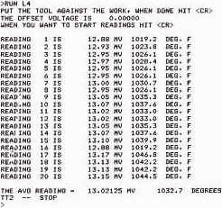
The program is written in FORTRAN and run on a DEC (Digital Equipment Corp.) PDP 11/34. The purpose of the program is to collect data on cutting temperature during a turning operation. A tool-chip thermocouple is used as the sensor. It uses the tool and the work material as the two dissimilar metals of the thermocouple. The millivolt output of the thermocouple is fed through an analog-to-digital converter into the computer. The thermocouple output
is sampled four times per second for 5 seconds. Then the 20 mV and temperature readings are printed out on a teletype, together with the averages of the 20 readings.
The program is shown in Figure 17.5 and a typical printout of results is displayed in Figure 17.6. The reader who is familiar with FORTRAN will recognize the structure and syntax of the statements. After the initializing statements (lines 1 through 8), the CALL ASICLN (LUN) in line 9 identifies the input unit assigned to the ADC. Literally, ASICLN(LUN) means “assign industrial controller to (logical unit number).” In line 10,
Figure 17.5 Process monitoring program of Example 17.5.
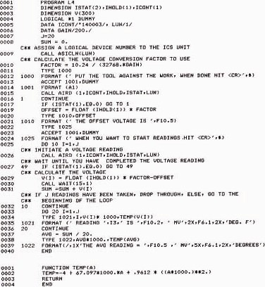
Figure 17.6 Output of process monitoring program of Example 17.5.
the program calculates the scale factor to use for the analog-to-digital converter (refer back to the discussion on ADCs in Section 17.4).
In lines 11 and 12, the program instructs the machine tool operator to “put the tool against the work, when done hit carriage return.” The statement in line 15,
Call Aird (1,Icont,Ihold,Istat,Lun)
commands the computer to accept the analog input from the ADC. This provides a zero set point for subsequent measurements taken during the cut. In lines 20 and 21, this value of the “offset voltage” is programmed to be printed.
The program then instructs the operator to start taking measurements with the statement: “When you want to start readings, hit carriage return.” Lines 25 through 32 comprise a DO loop which calls for the analog input (CALL AIRD) to be read and stored in a storage location called IHOLD. This is done for 20 cycles (J = 20 in line 7). The readings are taken at 1/4-s intervals. This is defined by the statement in line 30,
Call Watt (15,0)
This command makes the computer wait for 15 “ticks” before accepting the input. A “tick” in this computer system is l/60 s. Hence, 15 ticks equals lk s.
The remainder of the program is for printout of the data. Lines 33 to 36 print the 20 values of millivolt and corresponding cutting temperature values. The symbol V(I) is used for the 20 values of voltage. V(I) multiplied by 1000 converts the voltage measurements to
millivoltage for printout. The term TEMP(V(I)) calls a function for converting the voltage output of the tool-chip thermocouple into the corresponding temperature. The conversion is based on an equation that was derived from the calibration curve for the particular tool work material combination. In this case, the calibration equation is
TEMP = -4 + 67.097 MV + .9612(MV)2
where TEMP is the calculated cutting temperature and MV is thermocouple output. The function that performs this calculation is shown in Figure 17.5.
Lines 38 and 39 print the average values of millivolt and cutting temperature.
Figure 17.6 illustrates the output from the program during one cut of the turning operation. The teletype is located at the lathe, while the PDP 11/34 is remotely located in a separate room.
17.6 Hierarchical Computer Structures And Networking
Within some corporations, partially due to developments in computer-aided manufacturing, computer systems have grown to form pyramidlike structures in which computers at the industrial process level are linked to larger, more centralized systems, all the way up to the corporate computer.
In these heirarchical structures, information flows in two directions. Process monitoring data, production status information, and other operational data are passed upward through each level of computer system, and at each step, bulk information is filtered and integrated for more efficient use. In the reverse direction, commands and schedules are passed down from the corporate computer throughout the rest of the processing structure.
In this section we discuss the various functions performed at the different levels of the computer hierarchy. We also discuss the communication networks that connect these different levels.
Levels of computer hierarchy
Each level in the computer hierarchy exerts a certain amount of control over the activities performed in a manufacturing firm. The general structure of the system is depicted in Figure 17.7. The functions of these levels of control are described below.
In the first level of computer control, computers are connected directly to the manufacturing process. They are characteristically small, usually minicomputers or microcomputers. These computers are dedicated to process control and communicate only with systems in the second level of control.
Minicomputers make up the majority of systems in the second level of computer control. Usually, several minicomputers report to a larger plant computer.
Figure 17.7 Hierarchy of computers in manufacturing.
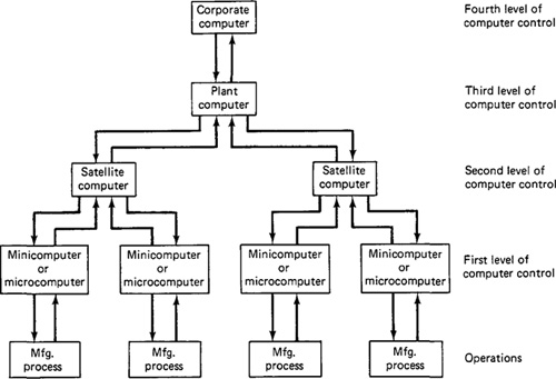
The minicomputers are often referred to as satellites of the larger computer. The minis serve to coordinate the activities of the smaller computers under them. Performance data from machine tools, for example, are collected from the first-level computers, and instructions are relayed back down the line to each process. This mode of operation is known as supervisory computer control, and is the basis for direct numerical control machining.
At the third level of control are the central plant computers, which collect data from the minicomputers beneath them in the structure, and prepare daily, weekly, and monthly reports using various information. Operating instructions are relayed to the second control level for implementation. Computers at this level are larger machines, and they are usually shared by many departments.
The corporate computer resides at the fourth level of control. Different plants report information to these computers, which then summarize the data and analyze plant operations and performance over a long-term period. The corporate computer is shared by departments such as marketing, engineering, and accounting.
Several important advantages can be claimed for the hierarchical computer structure in process control:
Control can be established gradually, with each application of computers justified on its own merits. An all-or-nothing commitment to an extensive computer system is not required, nor is the large expense of implementing such a system.
Redundancy in the hierarchical structure allows other computers to assume the functions of those which occasionally fail.
Software development in these structures is made more manageable in that programming projects can be undertaken independent of one another.
Computer network structures
The term “computer network” refers to the actual physical connections between computers in the structure. This structure consists not only of the computers, but also the terminals, transmission lines, switching centers, and other devices required to accomplish the desired functions of the system. The number of possible configurations is limitless. However, the various network arrangements divide themselves into several basic categories, sometimes called topologies. Four of the more common topologies are:
1. Point-to-point
2. Star network
3. Multidrop network
4. Loop configuration
These four network topologies are illustrated in Figure 17.8 and described in the paragraphs below.
In the point-to-point configuration, a communication line is established between two devices (typically, a computer and a peripheral device such as a terminal). It is a relatively simple configuration if the number of devices is limited. However, when there are a large number of processors in the structure, the number of point-to-point communication links can become significantly large, resulting in a relatively expensive system. Other network structures share the communication links in various ways to avoid this expense. An inherent advantage of the point-to-point configuration is that whenever one of the direct links is broken, the other connections remain intact.
The star network consists of a central computer and several peripheral devices connected to it. The central computer is referred to as the master and the peripherals are called slaves. The function of the master is to delegate tasks to each of the smaller units or to act as a switch to connect various units. One of the important deficiencies of the star configuration is that the entire network system is put out of operation if the central computer fails.
In the multidrop network structure, computers and other devices are connected by a single communication line. This line is either a bus or a serial channel. The limitation of this arrangement is that only two processors are allowed to transmit data to each other at the same time. This results from the shared nature of the communication lines.
In a loop configuration, each computer is connected to a communication line
Figure 17.8 Types of computer network structures: (a) point-to-point; (b) star; (c) multidrop; (d) loop.
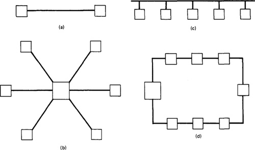
which begins and terminates at a loop controller, typically a computer that maintains control over intercomputer communications. Messages to a specific computer are usually transmitted to all computers in the network, with the addressee decoding its address and accepting the information.
References
[1] CADZOW, J. A., and MARTENS, H. R., Discrete-Time and Computer Control Systems, Prentice-Hall, Inc., Englewood Cliffs, N.J., 1970.
[2] ENG, E., “Peripheral Equipment for the Computer,” Electronic Engineering, November, 1978, pp. 107–116.
[3] GROOVER, M. P., Automation, Production System, and Computer-Aided Manufacturing, Prentice-Hall, Inc., Englewood Cliffs, N.J., 1980 Chapter 11.
[4] HARRISON, T. J. (Ed.), Minicomputers in Industrial Control, Instrument Society of America Pittsburgh, Pa., 1978.
[5] OFFORD, G., Personal communications and special reports, February/March, 1982.
[6] REMBOLD, U., SETH,M. K., and WEINSTEIN, J. S., Computers in Manufacturing, Marcel Dekker, Inc., New York, 1977.
[7] SCHAFFER, G., “Computers in Manufacturing,” Special Report 703, American Machinist, April, 1978, pp. 115–130.
Problems
17.1. An analog-to-digital converter is to be used to convert a continuous voltage signal into digital form. The full scale range is 110 V. An 8-bit ADC will be used. Determine the number of quantization levels, the resolution, and the spacing between adjacent quantization levels.
17.2. The selection of an analog-to-digital converter includes determining the number of bits required to achieve a certain level of precision in the converted signal. The incoming voltage signal has a full-scale range of 200 V, and it is desired to read that voltage to a spacing between adjacent quantization levels of 0.2 V. Determine the number of bits needed to provide this precision.
17.3. A successive approximation ADC is used to convert a 35.6-V signal into its equivalent digital value. A starting trial voltage of 80 V is used and the ADC possesses 8 bits of precision to accomplish the successive approximations. Construct a chart similar to that shown in Figure 17.3 and determine the final digital value as provided by the ADC.
17.4. A digital-to-analog converter uses a reference voltage of 100 V and its binary register contains eight-digit accuracy. At a particular sampling instant, the bit values in the register are as follows:
![]()
If a zero-order data-hold device is used, determine the value of the voltage during the time interval following this sampling instant.
17.5.A certain DAC uses a reference voltage of 100 V and an 8-bit binary register. In two successive sampling instants, the bit values in the register are as follows:
If a first-order hold is used in this DAC, determine the equation of the form of Eq. (17.4) which controls the voltage level during the interval following sampling instant t.
17.6.You have been asked to supervise a special engineering group whose function is to design and install a computer-aided manufacturing system for your company. The company consists of a corporate headquarters and two separate manufacturing plants located 25 miles apart. One plant manufactures in batches the basic components for the company’s products. It has 26 numerical control machine tools. The other plant is an assembly plant, which is also a warehouse and distribution center. In the style of a memorandum addressed to the company president, describe the hierarchical computer structure you would recommend. Allow for differences between the two plants. Define the type of information that would be communicated among the various levels of the computer heirarchy. What factors affect your recommendation? Sketch a diagram in the format of Figure 17.7 showing your recommended computer system.