Chapter 11. Memory
Chapter Objectives
After reading this chapter, you’ll be able to do the following:
• Read from and write to memory from shaders.
• Perform simple mathematical operations directly on memory from shaders.
• Synchronize and communicate between different shader invocations.
Everything in the OpenGL pipeline thus far has essentially been side-effect free. That is, the pipeline is constructed from a sequence of stages, either programmable (such as the vertex and fragment shaders) or fixed function (such as the tessellation engine) with well-defined inputs and outputs (such as vertex attributes or color outputs to a framebuffer). Although it has been possible to read from arbitrary memory locations using textures or texture buffer objects (TBOs), in general, writing has been allowed only to fixed and predictable locations. For example, vertices captured during transform feedback operations are written in well-defined sequences to transform feedback buffers, and pixels produced in the fragment shader are written into the framebuffer in a regular pattern defined by rasterization.
This chapter introduces mechanisms by which shaders may both read from and write to user-specified locations. This allows shaders to construct data structures in memory and, by carefully updating the same memory locations, effect a level of communication between each other. To this end, we also introduce special functions both in the shading language and in the OpenGL API that provide control over the order of access and of the operations performed during those memory accesses.
This chapter has the following major sections:
• “Using Textures for Generic Data Storage” shows how to read and write memory held in a texture object through GLSL built-in functions.
• “Shader Storage Buffer Objects” shows how to read and write a generic memory buffer directly through user-declared variables.
• “Atomic Operations and Synchronization” explains multiple-writer synchronization problems with images and how to solve them.
• “Example: Order-Independent Transparency” discusses an interesting use of many of the features outlined in the chapter in order to demonstrate the power and flexibility that generalized memory access provides to the experienced OpenGL programmer.
Using Textures for Generic Data Storage
It is possible to use the memory representing a buffer object or a single level of a texture object for general-purpose read and write access in shaders. To support this, the OpenGL Shading Language provides several image types to represent raw image data.
Images are declared in shaders as uniforms in a similar manner to samplers. Just like samplers, they are assigned locations by the shader compiler that can be passed to glUniform1i()to specify the image unit which they represent. The OpenGL Shading Language image types are shown in Table 11.1.

Notice that most of the GLSL sampler types have an analogue as an image type. The primary differences between a sampler type (such as sampler2D) and an image type (such as image2D) are first, that the image type represents a single layer of the texture, not a complete mipmap chain and second, that image types do not support sampler operations such as filtering. These unsupported sampling operations include depth comparison, which is why the shadow sampler types such as sampler2DShadow do not have an equivalent image type.
The three basic classes of image types—image*, iimage*, and uimage*—are used to declare images containing floating-point, signed integer, or unsigned integer data, respectively.
In addition to the general data type (floating-point, signed, or unsigned integer) associated with the image variable, a format layout qualifier may be given to further specify the underlying image format of the data in memory. Any image from which data will be read must be declared with a format layout qualifier, but in general, it is a good idea to explicitly state the format of the data in the image at declaration time. The format layout qualifiers and their corresponding OpenGL internal format types are shown in Table 11.2.
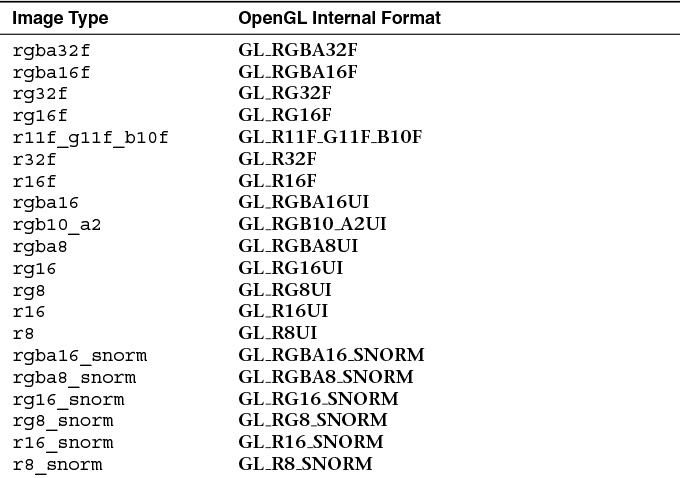
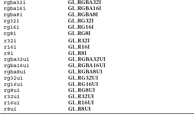
The image format qualifier is provided as part of the image variable declaration and must be used when declaring an image variable that will be used to read from an image. It is optional if the image will only ever be written to. (See the explanation of writeonly for more details.) The image format qualifier used in the declaration of such variables (if present) must batch the basic data type of the image. That is, floating-point format specifiers such as r32f or rgba16_snorm must be used with floating-point image variables such as image2D, while non-floating-point qualifiers (such as rg8ui) may not. Likewise, signed integer format qualifiers such as rgba32i must be used to declare signed integer image variables (iimage2D), and unsigned format qualifiers (rgba32ui) must be used to declare unsigned integer image variables (uimage2D).
Examples of using the format layout qualifiers to declare image uniforms are shown in Example 11.1.
Example 11.1 Examples of Image Format Layout Qualifiers
// 2D image whose data format is 4-component floating-point
layout (rgba32f) uniform image2D image1;
// 2D image whose data format is 2-component integer
layout (rg32i) uniform iimage2D image2;
// 1D image whose data format is single-component unsigned integer
layout (r32ui) uniform uimage1D image3;
// 3D image whose data format is single-component integer and is
// initialized to refer to image unit 4
layout (binding=4, r32) uniform iimage3D image4;
The format type used in the declaration of the image variable does not need to match the underlying format of the data in the image (as given by the texture’s internal format), but it should be compatible as defined by the OpenGL specification. In general, if the amount of data storage required per texel is the same between two formats, the formats are considered to be compatible. For example, a texture whose internal format is GL_RGBA32F has four, 32-bit (floating-point) components, for a total of 128 bits per texel. Levels of this texture may be accessed in a shader through image variables whose format is rgba32f, rgba32ui, or rgba32i, as all of these formats represent a single texel using 128 bits. Furthermore, a texture whose internal format is GL_RG16F is represented as 32 bits per texel. This type of texture may be accessed using image variables declared as r32f, rgba8ui, rgb10_a2ui, or any other format that represents a texel using 32 bits. When texture and image variable formats do not match but are otherwise compatible, the raw data in the image is reinterpreted as the type specified in the shader. For example, reading from a texture with the GL_R32F internal format using an image variable declared as r32ui will return an unsigned integer whose bit pattern represents the floating-point data stored in the texture.
The maximum number of image uniforms that may be used in a single shader stage may be determined by querying the value of GL_MAX_VERTEX_IMAGE_UNIFORMS for vertex shaders, GL_MAX_TESS_CONTROL_IMAGE_UNIFORMS, and GL_MAX_TESS_EVALUATION_IMAGE_UNIFORMS for tessellation control and evaluation shaders, respectively; GL_MAX_GEOMETRY_IMAGE_UNIFORMS for geometry shaders; and finally, GL_MAX_FRAGMENT_IMAGE_UNIFORMS for fragment shaders. Additionally, the maximum number of image uniforms that may be used across all active shaders is given by GL_MAX_COMBINED_IMAGE_UNIFORMS. In addition to these limits, some implementations may have restrictions upon the number of image uniforms available to a fragment shader when that shader also writes to the framebuffer using traditional output variables. To determine whether this is the case, retrieve the value of GL_MAX_COMBINED_IMAGE_UNITS_AND_FRAGMENT_OUTPUTS. A final note is that although the OpenGL API supports image uniforms in every shader stage, it mandates only that implementations provide support in the fragment shader and that only GL_MAX_FRAGMENT_IMAGE_UNIFORMS be nonzero.
Binding Textures to Image Units
Just as sampler variables represent texture units in the OpenGL API, so do image variables represent a binding to an image unit in the OpenGL API. Image uniforms declared in a shader have a location that may be retrieved by calling glGetUniformLocation(). This is passed in a call go glUniform1i()to set the index of the image unit to which the image uniform refers. This binding may also be specified directly1 in the shader using a binding layout qualifier as shown in the declaration of image4 in Example 11.1. By default, an image uniform has the binding 0, so if only one image is used in a shader, there is no need to explicitly set its binding to 0. The number of image units supported by the OpenGL implementation may be determined by retrieving the value of GL_MAX_IMAGE_UNITS. A single layer of a texture object must be bound to an image unit before it can be accessed in a shader. To do this, call glBindImageTexture(), whose prototype is as follows:
1. The option of specifying the image unit in the shader using the binding layout qualifier is generally preferred. This is because some OpenGL implementations may provide a multithreaded shader compiler. If properties of a linked program, such as the locations of uniforms, are queried too soon after the program is linked, the implementation may need to stall to allow compilation and linking to complete before it can return. By specifying the bindings explicitly, the uniform location query and the potential stall may be avoided.
Texture objects that will be used for generic memory access are created and allocated as usual by calling glCreateTextures() and one of the texture allocation functions, such as glTextureSubImage2D() or glTextureStorage3D(). Once created and allocated, they are bound to an image unit using glBindImageTexture() for read, write, or both read and write access, as specified by the access parameter to glBindImageTexture(). Violating this declaration (for example, by writing to an image bound using GL_READ_ONLY for access) will cause undesired behavior, possibly crashing the application.
An example of creating, allocating, and binding a texture for read and write access in shaders is given in Example 11.2.
Example 11.2 Creating, Allocating, and Binding a Texture to an Image Unit
GLuint tex;
// Generate a new name for our texture
glCreateTextures(1, GL_TEXTURE_2D, &tex);
// Allocate storage for the texture
glTextureStorage2D(tex, 1, GL_RGBA32F, 512, 512);
// Now bind it for read-write to one of the image units
glBindImageTexture(0, tex, 0, GL_FALSE, 0, GL_READ_WRITE, GL_RGBA32F);
glBindImageTexture() works similarly to glBindTextureUnit(). There is, however, a small difference. The format in which formatted stores (writes from the shader) will be performed is specified during the API call. This format should match the format of the image uniform in the shaders that will access the texture. However, it need not match the format of the actual texture. For textures allocated by calling one of the glTexImage() or glTexStorage() functions, any format that matches in size may be specified for format. For example, formats GL_R32F, GL_RGBA8, and GL_R11F_G11F_B10F are all considered to consist of 32 bits per texel and therefore to match in size. A complete table of all of the sizes of the texture formats is given in the OpenGL specification.
To use a buffer object as the backing store for an imageBuffer image in a shader, it must still be represented as a texture by creating a buffer texture, attaching the buffer object to the texture object, and then binding the buffer texture to the image unit as shown in Example 11.3. The format of the data in the buffer object is specified when it is attached to the texture object. The same buffer may be attached to multiple texture objects simultaneously with different formats, allowing some level of format aliasing to be implemented.
Example 11.3 Creating and Binding a Buffer Texture to an Image Unit
GLuint tex;
Gluint buf;
// Generate a name for the buffer object
glCreateBuffers(1, &buf);
// Allocate storage for the buffer object - 4K here
glNamedBufferStorage(buf, 4096, nullptr, 0);
// Generate a new name for our texture
glCreateTextures(1, GL_TEXTURE_BUFFER, &tex);
// Attach the buffer object to the texture and specify format as
// single-channel floating-point
glTextureBuffer(tex, GL_R32F, buf);
// Now bind it for read-write to one of the image units
glBindImageTexture(0, tex, 0, GL_FALSE, 0, GL_READ_WRITE, GL_RGBA32F);
Reading and Writing to Images
Once an image has been declared in the shader and a level and layer of a texture have been bound to the corresponding image unit, the shader may access the data in the texture directly for both read and write. Reading and writing are done only through built-in functions that load or store their arguments to or from an image. To load texels from an image, call imageLoad(). There are many overloaded variants of imageLoad(). They are as follows:
The imageLoad() functions operate similarly to texelFetch(), which is used to directly read texels from textures without any filtering applied. In order to store into images, the imageStore() function may be used. imageStore() is defined as follows:
If you need to know the size of an image in the shader, you can query with these imageSize() functions:
Example 11.4 shows a simple but complete example of a fragment shader that performs both image loads and stores from and to multiple images. It also performs multiple stores per invocation.
Example 11.4 Simple Shader Demonstrating Loading and Storing into Images
#version 420 core
// Buffer containing a palette of colors to mark primitives by ID
layout (binding = 0, rgba32f) uniform imageBuffer colors;
// The buffer that we will write to
layout (binding = 1, rgba32f) uniform image2D output_buffer;
out vec4 color;
void main(void)
{
// Load a color from the palette based on primitive ID % 256
vec4 col = imageLoad(colors, gl_PrimitiveID & 255);
// Store the resulting fragment at two locations: first at the
// fragment’s window space coordinate shifted left...
imageStore(output_buffer,
ivec2(gl_FragCoord.xy) - ivec2(200, 0), col);
// ... then at the location shifted right
imageStore(output_buffer,
ivec2(gl_FragCoord.xy) +ivec2(200, 0), col);
}
The shader in Example 11.4 loads a color from a buffer texture indexed by a function of gl_PrimitiveID and then writes it twice into a single image indexed by functions of the current two-dimensional fragment coordinate.
Notice that the shader has no other per-fragment outputs. The result of running this shader on some simple geometry is shown in Figure 11.1.

As can be seen in Figure 11.1, two copies of the output geometry have been rendered: one in the left half of the image and the other in the right half of the image. The data in the resulting texture was explicitly placed with the shader of Example 11.4. While this may seem like a minor accomplishment, it actually illustrates the power of image store operations. It demonstrates that a fragment shader is able to write to arbitrary locations in a surface. In traditional rasterization into a framebuffer, the location at which the fragment is written is determined by fixed function processing before the shader executes. However, with image stores, this location is determined by the shader. Another thing to consider is that the number of stores to images is not limited, whereas the number of attachments allowed on a single framebuffer object is, and only one fragment is written to each attachment. This means that a much larger amount of data may be written by a fragment shader using image stores than would be possible using a framebuffer and its attachments. In fact, an arbitrary amount of data may be written to memory by a single shader invocation using image stores.
Figure 11.1 also demonstrates another facet of stores from shaders. That is they are unordered and can be subject to race conditions. The program that generated the image disabled both depth testing and back-face culling, meaning that each pixel has at least two primitives rendering into it. The speckled corruption that can be seen in the image is the result of the nondeterministic order with which the primitives are rendered by OpenGL. We will cover race conditions and how to avoid them later in this chapter.
Shader Storage Buffer Objects
Reading data from and writing data to memory using image variables works well for simple cases where large arrays of homogeneous data are needed or the data is naturally image-based (such as the output of OpenGL rendering or where the shader is writing into an OpenGL texture). However, in some cases, large blocks of structured data may be required. For these use cases, we can use a buffer variable to store the data. Buffer variables are declared in shaders by placing them in an interface block, which in turn is declared using the buffer keyword. A simple example is given in Example 11.5.
Example 11.5 Simple Declaration of a Buffer Block
#version 430 core
// create a readable-writable buffer
layout (std430, binding = 0) buffer BufferObject {
int mode; // preamble members
vec4 points[]; // last member can be unsized array
};
In addition to declaring the interface block BufferObject as a buffer block, Example 11.5 includes two further layout qualifiers attached to the block. The first, std430, indicates that the memory layout of the block should follow the std430 standard, which is important if you want to read the data produced by the shader in your application, or possibly generate data in the application and then consume it from the shader. The std430 layout is documented in Appendix H, “Buffer Object Layouts,” and is similar to the std140 layout used for uniform blocks but a bit more economical with its use of memory.
The second qualifier, binding = 0, specifies that the block should be associated with the GL_SHADER_STORAGE_BUFFER binding at index zero. Declaring an interface block using the buffer keyword indicates that the block should be stored in memory and backed by a buffer object. This is similar to how a uniform block is backed by buffer object bound to one of the GL_UNIFORM_BUFFER indexed binding points. The big difference between a uniform buffer and a shader storage buffer is that the shader storage buffer can both be read and written from the shader. Any writes to the storage buffer via a buffer block will eventually be seen by other shader invocations and can be read back by the application.
An example of how to initialize a buffer object and bind it to one of the indexed GL_SHADER_STORAGE_BUFFER bindings is shown in Example 11.6.
Example 11.6 Creating a Buffer and Using It for Shader Storage
GLuint buf;
// Generate the buffer, bind it to create it, and declare storage
glGenBuffers(1, &buf);
glBindBuffer(GL_SHADER_STORAGE_BUFFER, buf);
glBufferData(GL_SHADER_STORAGE_BUFFER, 8192, NULL, GL_DYNAMIC_COPY);
// Now bind the buffer to the zeroth GL_SHADER_STORAGE_BUFFER
// binding point
glBindBufferBase(GL_SHADER_STORAGE_BUFFER, 0, buf);
Writing Structured Data
In the beginning of the section, we mentioned reading and writing structured data. If all you had was an array of vec4, you probably could get by with using image buffers. However, if you really have a collection of structured objects, where each is heterogeneous collection of types, image buffers would become quite cumbersome. With shader storage buffers, however, you get full use of GLSL structure definitions and arrays to define the layout of your buffer. See the example in Example 11.7 to get the idea.
Example 11.7 Declaration of Structured Data
#version 430 core
// structure of a single data item
struct ItemType {
int count;
vec4 data[3];
// ... other fields
};
// declare a buffer block using ItemType
layout (std430, binding = 0) buffer BufferObject {
// ... other data here
ItemType items[]; // render-time sized array of items typed above
};
As you see existing examples of using images to play the role of accessing memory, it will be easy to imagine smoother sailing through the more direct representation enabled by using buffer blocks (shader storage buffer objects).
Atomic Operations and Synchronization
Now that you have seen how shaders may read and write arbitrary locations in textures (through built-in functions) and buffers (through direct memory access), it is important to understand how these accesses can be controlled such that simultaneous operations to the same memory location do not destroy each other’s effects. In this section, you will be introduced to a number of atomic operations that may be performed safely by many shader invocations simultaneously on the same memory location. Also, we will cover functionality that allows your application to provide ordering information to OpenGL. This to ensure that reads observe the results of any previous writes and that writes occur in desired order, leaving the correct value in memory.
Atomic Operations on Images
The number of applications for simply storing randomly into images and buffers is limited. However, GLSL provides many more built-in functions for manipulating images. These include atomic functions that perform simple mathematical operations directly on the image in an atomic fashion. Atomic operations (or atomics) are important in these applications because multiple shader instances could attempt to write to the same memory location. OpenGL does not guarantee the order of operations for shader invocations produced by the same draw command or even between invocations produced by separate drawing commands. It is this undefined ordering that allows OpenGL to be implemented on massively parallel architectures and provide extremely high performance. However, this also means that the fragment shader might be run on multiple fragments generated from a single primitive or even fragments making up multiple primitives simultaneously. In some cases, different fragment shader invocations could literally access the same memory location at the same instant in time, could run out of order with respect to one another, or could even pass each other in execution order. As an example, consider the naïve shader shown in Example 11.8.
Example 11.8 Naïvely Counting Overdraw in a Scene
#version 420 core
// This is an image that will be used to count overdraw in the scene.
layout (r32ui) uniform uimage2D overdraw_count;
void main(void)
{
// Read the current overdraw counter
uint count = imageLoad(overdraw_count, ivec2(gl_FragCoord.xy));
// Add one
count = count + 1;
// Write it back to the image
imageStore(output_buffer, ivec2(gl_FragCoord.xy), count);
}
The shader in Example 11.8 attempts to count overdraw in a scene. It does so by storing the current overdraw count for each pixel in an image. Whenever a fragment is shaded, the current overdraw count is loaded into a variable, incremented, and then written back into the image. This works well when there is no overlap in the processing of fragments that make up the final pixel. However, when image complexity grows and multiple fragments are rendered into the final pixel, strange results will be produced. This is because the read-modify-write cycle performed explicitly by the shader can be interrupted by another instance of the same shader. Take a look at the timeline shown in Figure 11.2.

Figure 11.2 shows a simplified timeline of four fragment shader invocations running in parallel. Each shader is running the code in Example 11.8 and reads a value from memory, increments it, and then writes it back to memory over three consecutive time steps. Now consider what happens if all four invocations of the shader end up accessing the same location in memory. At time 0, the first invocation reads the memory location; at time 1, it increments it; and at time 2, it writes the value back to memory. The value in memory (shown in the rightmost column) is now 1, as expected. Starting at time 3, the second invocation of the shader (fragment 1) executes the same sequence of operations—load, increment, and write, over three time steps. The value in memory at the end of time step 5 is now 2, again as expected.
Now consider what happens during the third and fourth invocations of the shader. In time step 6, the third invocation reads the value from memory (which is currently 2) into a local variable, and at time step 7, it increments the variable, ready to write it back to memory. However, also during time step 7, the fourth invocation of the shader reads the same location in memory (which still contains the value 2) into its own local variable. It increments that value in time step 8 while the third invocation writes its local variable back to memory. Memory now contains the value 3. Finally, the fourth invocation of the shader writes its own copy of the value into memory in time step 9. However, because it read the original value in time step 7—after the third invocation had read from memory but before it had written the updated value back—the data written is stale. The value of the local variable in the fourth shader invocation is 3 (the stale value plus 1), not 4, as might be expected. The desired value in memory is 4, not 3, and the result is the blocky corruption shown in Figure 11.3.

The reason for the corruption in this example is that the increment operations performed by the shader are not atomic with respect to each other. That is, they do not operate as a single, indivisible operation but as a sequence of independent operations that may be interrupted or may overlap with the processing performed by other shader invocations accessing the same resources. Although this simple explanation describes only the hypothetical behavior of four invocations, when considering that modern GPUs typically have hundreds or even thousands of concurrently executing invocations, it becomes easy to see how this type of issue is encountered more often than one would imagine.
To avoid this, OpenGL provides a set of atomic functions that operate directly on memory. They have two properties that make them suitable for accessing and modifying shared memory locations. First, they apparently operate in a single time step2 without interruption by other shader invocations, and second, the graphics hardware provides mechanisms to ensure that even if multiple concurrent invocations perform an atomic operation on the same memory location at the same instant, they will appear to be serialized such that they take turns executing and produce the expected result. Note that there is still no guarantee of order—just a guarantee that all invocations execute their operation without stepping on each other’s results.
2. This may not actually be true: They could take several tens of clock cycles, but the graphics hardware will make them appear to be single, indivisible operations.
The shader in Example 11.8 may be rewritten using an atomic function as shown in Example 11.9. In Example 11.9, the imageAtomicAdd function is used to directly add one to the value stored in memory. This is executed by OpenGL as a single, indivisible operation and therefore isn’t susceptible to the issues illustrated in Figure 11.2.
Example 11.9 Counting Overdraw with Atomic Operations
#version 420 core
// This is an image that will be used to count overdraw in the scene.
layout (r32ui) uniform uimage2D overdraw_count;
void main(void)
{
// Atomically add one to the contents of memory
imageAtomicAdd(overdraw_count, ivec2(gl_FragCoord.xy), 1);
}
The result of executing the shader shown in Example 11.9 is shown in Figure 11.4. As you can see, the output is much cleaner.

imageAtomicAdd is one of many atomic built-in functions in GLSL. These functions include addition and subtraction, logical operations, and comparison and exchange operations. This is the complete list of GLSL atomics:
In the declarations of the atomic image functions, IMAGE_PARAMS may be replaced with any of the definitions given in Example 11.10. The effect of this is that there are several overloaded versions of each of the atomic functions.
Example 11.10 Possible Definitions for IMAGE_PARAMS
#define IMAGE_PARAMS gimage1D image, int P // or
#define IMAGE_PARAMS gimage2D image, ivec2 P // or
#define IMAGE_PARAMS gimage3D image, ivec3 P // or
#define IMAGE_PARAMS gimage2DRect image, ivec2 P // or
#define IMAGE_PARAMS gimageCube image, ivec3 P // or
#define IMAGE_PARAMS gimageBuffer image, int P // or
#define IMAGE_PARAMS gimage1DArray image, ivec2 P // or
#define IMAGE_PARAMS gimage2DArray image, ivec3 P // or
#define IMAGE_PARAMS gimageCubeArray image, ivec3 P // or
#define IMAGE_PARAMS gimage2DMS image, ivec2 P, int sample // or
#define IMAGE_PARAMS gimage2DMSArray image, ivec3 P, int sample
Atomic functions can operate on single signed or unsigned integers. That is, neither floating-point images nor images of vectors of any type are supported in atomic operations. Each atomic function returns the value that was previously in memory at the specified location. If this value is not required by the shader, it may be safely ignored. Shader compilers may then perform data-flow analysis and eliminate unnecessary memory reads if it is advantageous to do so. As an example, the equivalent code for imageAtomicAdd is given in Example 11.11. Although Example 11.11 shows imageAtomicAdd implemented as several lines of code, it is important to remember that this is for illustration only and that the built-in imageAtomicAdd function operates as a single, indivisible operation.
Example 11.11 Equivalent Code for imageAtomicAdd
// THIS FUNCTION OPERATES ATOMICALLY
uint imageAtomicAdd(uimage2D image, ivec2 P, uint data)
{
// Read the value that's currently in memory
uint val = imageLoad(image, P).x;
// Write the new value to memory
imageStore(image, P, uvec4(val + data));
// Return the *old* value.
return val;
}
As has been shown in Example 11.9, this atomic behavior may be used to effectively serialize access to a memory location. Similar functionality for other operations such as logical operations is achieved through the use of imageAtomicAnd, imageAtomicXor, and so on. For example, two shader invocations may simultaneously set different bits in a single memory location using the imageAtomicOr function. The two atomic functions that do not perform arithmetic or logical operations on memory are imageAtomicExchange and imageAtomicCompSwap. imageAtomicExchange is similar to a regular store except that it returns the value that was previously in memory. In effect, it exchanges the value in memory with the value passed to the function, returning the old value to the shader. imageAtomicCompSwap is a generic compare-and-swap operation that conditionally stores the specified data in memory. The equivalent code for these functions is shown in Example 11.12.
Example 11.12 Equivalent Code for imageAtomicExchange and imageAtomicComp
// THIS FUNCTION OPERATES ATOMICALLY
uint imageAtomicExchange(uimage2D image, ivec2 P, uint data)
{
uint val = imageLoad(image, P);
imageStore(image, P, data);
return val;
}
// THIS FUNCTION OPERATES ATOMICALLY
uint imageAtomicCompSwap(uimage2D image, ivec2 P,
uint compare, uint data)
{
uint val = imageLoad(image, P);
if (compare == val)
{
imageStore(image, P, data);
}
return val;
}
Again, it is important to remember that the code given in Example 11.12 is for illustrative purposes only and that the imageAtomicExchange and imageAtomicCompSwap functions are truly implemented using hardware support as opposed to a sequence of lower-level operations. One of the primary use cases for imageAtomicExchange is in the implementation of linked lists or other complex data structures. In a linked list, the head and tail pointers may be swapped with references to new items inserted into the list atomically to effectively achieve parallel list insertion. Likewise, imageAtomicCompSwap may be used to implement locks (also known as mutexes) to prevent simultaneous access to a shared resource (such as another image). An example of taking a lock using an atomic compare-and-swap operation (as implemented by imageAtomicCompSwap) is shown in Example 11.13.
Example 11.13 Simple Per-Pixel Mutex Using imageAtomicCompSwap
#version 420 core
layout (r32ui) uniform uimage2D lock_image;
layout (rgba8f) uniform image2D protected_image;
void takeLock(ivec2 pos)
{
int lock_available;
do {
// Take the lock - the value in lock_image is 0 if the lock
// is not already taken. If so, it is overwritten with
// 1 otherwise it is left alone. The function returns the value
// that was originally in memory - 0 if the lock was not taken,
// 1 if it was. We terminate the loop when we see that the lock
// was not already taken and thus we now hold it because we've
// written a one to memory.
lock_available = imageAtomicCompSwap(lock_image, pos, 0, 1);
} while (lock_available == 0);
}
void releaseLock(ivec2 pos)
{
imageStore(lock_image, pos, 0);
}
void operateOnFragment()
{
// Perform a sequence of operations on the current fragment
// that need to be indivisible. Here, we simply perform
// multiplication by a constant as there is no atomic version
// of this (imageAtomicMult, for example). More complex functions
// could easily be implemented.
vec4 old_fragment;
old_fragment = imageLoad(protected_image,
ivec2(gl_FragCoord.xy));
imageStore(protected_image,
ivec2(gl_FragCoord.xy),
old_fragment * 13.37);
}
void main(void)
{
// Take a per-pixel lock
takeLock(ivec2(gl_FragCoord.xy));
// Now we own the lock and can safely operate on a shared resource
operateOnPixel();
// Be sure to release the lock...
releaseLock(ivec2(gl_FragCoord.xy));
}
The code shown in Example 11.13 implements a simple per-pixel mutex using the imageAtomicCompSwap function. To do this, it compares the value already in memory to zero (the third parameter to imageAtomicCompSwap). If they are equal (i.e., if the current value in memory is zero), it writes the new value (one, here) into memory. imageAtomicCompSwap then returns the value that was originally in memory. That is, if the lock was not previously taken, the value in memory will be zero (which is what is returned), but this will be replaced with one, reserving the lock. If the lock was previously taken by another shader invocation, the value in memory will already be one, and this is what will be returned. Therefore, we know that we received the lock when imageAtomicCompSwap returns zero. This loop, therefore, executes until imageAtomicCompSwap returns zero, indicating that the lock was available. When it does, this shader invocation will have the lock. The first invocation (after serialization by the hardware) that receives a zero from imageAtomicComSwap will hold the lock until it places a zero back into memory (which is what releaseLock does). All other invocations will spin in the loop in takeLock. They will be released from this loop one at a time until all invocations have taken the lock, performed their operations, and then released again.
The functionality implemented in operateOnFragment can be anything. It does not have to use atomics because the whole function is running while the lock is taken by the current shader invocation. For example, programmable blending3 operations could be implemented here by using imageLoad and imageStore to read and write a texture. Also, operations for which there is no built-in atomic function can be implemented. For example, multiplication, arithmetic shift, or transcendental functions can be performed on images.
3. Note that there is still no ordering guarantee, so only blending operations that are order-independent can be implemented here. A more complete example that includes order-independent blending is given at the end of this chapter.
Atomic Operations on Buffers
In addition to the atomic operations that may be performed on images, atomic operations may be performed on buffer variables. Buffer variables are variables inside interface blocks that have been declared with the buffer keyword. As with images, several built-in functions to perform atomic operations are defined. The atomic operations that may be performed on buffer variables are the same set that may be performed on image variables.
Each of these atomic functions takes an inout parameter that serves as a reference to a memory location. The value passed to any of these atomic functions in the mem parameter must4 be a member of a block declared with the buffer keyword. Like the image atomic functions, each of these functions returns the value originally in memory before it was updated. This effectively allows you to swap the content of memory for a new value, possibly conditionally, as in the case of atomicCompSwap.
4. Actually, these atomic functions may also be used on variables declared as shared. This will be discussed further in “Compute Shaders” in Chapter 12.
Sync Objects
OpenGL operates in a client-server model, where a server operates asynchronously to the client. Originally, this allowed the user’s terminal to render high-performance graphics and for the application to run on a server in a remote location. This was an extension of the X protocol, which was always designed with remote rendering and network operations in mind. In modern graphics workstations, we have a similar arrangement, with a slightly different interpretation. Here, the client is the CPU and the application runs on it, sending commands to the server, which is a high-performance GPU. However, the bandwidth between the two is still relatively low compared to the throughput and performance of either one. Therefore, for maximum performance, the GPU runs asynchronously to the CPU and can often be several OpenGL commands behind the application.
In some circumstances, it is necessary, however, to ensure that the client and the server—the CPU and the GPU—execute in a synchronized manner. To achieve this, we can use a sync object, which can also be known as a fence. A fence is essentially a marker in the stream of commands that can be sent along with drawing and state change commands to the GPU. The fence starts life in an unsignaled state and becomes signaled when the GPU has executed it. At any given time, the application can look at the state of the fence to see whether the GPU has reached it yet, and it can wait for the GPU to have executed the fence before moving on. To inject a fence into the OpenGL command stream, call glFenceSync():
When you call glFenceSync(), a new fence sync object is created, and the corresponding fence is inserted into the OpenGL command stream. The sync starts of unsignaled and will eventually become signaled when the GPU processes it. Because (although asynchronous) OpenGL has a well-defined order of execution, when a fence becomes signaled, you know that any commands that precede it in the command stream have finished executing, although nothing is known about commands that follow. To check whether a fence has been executed by the GPU you can call glGetSynciv():
To check whether a fence object has become signaled call glGetSynciv() with pname set to GL_SYNC_STATUS. Assuming that no error is generated and the buffer is big enough, either GL_SIGNALED or GL_UNSIGNALED will be written into the buffer pointed to by values, depending on whether the fence had been reached by the GPU. You can use this to poll a sync object to wait for it to become signaled, but this can be quite inefficient, with control passing backward between your application and the OpenGL implementation, and with all the error checking and other validation that the OpenGL drivers might do on your system occurring for each transition. If you wish to wait for a sync object to become signaled, you should call glClientWaitSync():
The glClientWaitSync() function is used to wait in the client for a fence to be reached by the server. It will wait for up to timeout nanoseconds for the sync object given by sync to become signaled before giving up. If flags contains GL_SYNC_FLUSH_COMMANDS_BIT, glClientWaitSync() will implicitly send any pending commands to the server before beginning to wait. It’s a good idea to set this bit, as without it the OpenGL driver might buffer up commands and never send them to the server, ensuring that your call to glClientWaitSync() will generate a timeout. glClientWaitSync() will generate one of four return values:
• GL_ALREADY_SIGNALED is returned if sync was already signaled when the call to glClientWaitSync() was made.
• GL_TIMEOUT_EXPIRED is returned if sync did not enter the signaled state before nanoseconds has passed.
• GL_CONDITION_SATISFIED is returned if sync was not signaled when the call to glClientWaitSync() was made but became signaled before nanoseconds has elapsed.
• GL_WAIT_FAILED is returned if the call to glClientWaitSync() failed for some reason, such as sync not being the name of a sync object. In this case, a regular OpenGL error is also generated and should be checked with glGetError(). Furthermore, if you are using a debug context, there is a good chance that its log will tell you exactly what went wrong.
Sync objects can only go from the unsignaled state (which is the state that they are created in) into the signaled state. Thus, they are basically single-use objects. Once you have finished waiting for a sync object, or if you decide you don’t need it any more, you should delete the sync object. To delete a sync object, call glDeleteSync():
A common use-case for sync objects is to ensure that the GPU is done using data in a mapped buffer before overwriting the data. This can occur if the buffer (or a range of it) was mapped using the glMapNamedBufferRange() function with the GL_MAP_UNSYNCHRONIZED_BIT set. This causes OpenGL to not wait for any pending commands that may be about to read from the buffer to complete before handing your application a pointer to write into. Under some circumstances, this pointer may actually address memory that the GPU is about to use. To make sure that you don’t stomp all over data that hasn’t been used yet, you can insert a fence right after the last command that might read from a buffer and then issue a call to glClientWaitSync() right before you write into the buffer. Ideally, you’d execute something that takes some time between the call to glFenceSync() and the call to glClientWaitSync(). A simple example is shown in Example 11.14.
Example 11.14 Example Use of a Sync Object
// This will be our sync object.
GLsync s;
// Bind a vertex array and draw a bunch of geometry
glBindVertexArray(vao);
glDrawArrays(GL_TRIANGLES, 0, 30000);
// Now create a fence that will become signaled when the
// above drawing command has completed
s = glFenceSync();
// Map the uniform buffer that's in use by the above draw
void * data = glMapNamedBufferRange(uniform_buffer,
0, 256,
GL_WRITE_BIT |
GL_MAP_UNSYNCHRONIZED_BIT);
// Now go do something that will last a while...
// ... say, calculate the new values of the uniforms
do_something_time_consuming();
// Wait for the sync object to become signaled.
// 1,000,000 ns = 1 ms.
glClientWaitSync(s, 0, 1000000);
// Now write over the uniform buffer and unmap it, and
// then delete the sync object.
memcpy(data, source_data, source_data_size);
glUnmapNamedBuffer(uniform_buffer);
glDeleteSync(s);
As with many other object types in OpenGL, it is possible to simply ask whether the object you have is what you think it is. To find out whether an object is a valid sync object, you can call glIsSync():
Advanced
If you are sharing objects between two or more contexts, it is possible to wait in one context for a sync object to become signaled as the result of commands issued in another. To do this, call glFenceSync() in the source context (the one which you want to wait on) and then call glWaitSync() in the destination context (the one that will do the waiting). The prototype for glWaitSync() is as follows:
glWaitSync() presents a rather limited form of what may be achieved with glClientWaitSync(). The major differences are the GL_SYNC_FLUSH_COMMANDS_BIT flag is not accepted in the flags parameter (nor is any other flag), and the timeout is implementation defined. You still have to ask for this implementation-defined timeout value by passing GL_TIMEOUT_IGNORED in timeout. However, you can find out what that implementation-dependent timeout value is by calling glGetIntegerv() with the parameter GL_MAX_SERVER_WAIT_TIMEOUT.
An example use for glWaitSync() synchronizing two contexts is when you are writing data into a buffer using transform feedback and want to consume that data in another context. In this case, you would issue the drawing commands that would ultimately update the transform feedback buffer and then issue the fence with a call to glFenceSync(). Next, switch to the consuming thread (either with a true context switch or by handing control to another application thread) and then wait on the fence to become signaled by calling glWaitSync() before issuing any drawing commands that might consume the data.
Image Qualifiers and Barriers
The techniques outlined thus far work well when compilers don’t perform overly aggressive optimizations on your shaders. However, under certain circumstances, the compiler might change the order or frequency of image loads or stores, and may eliminate them altogether if it believes they are redundant. For example, consider the simple example loop in Example 11.15.
Example 11.15 Basic Spin-Loop Waiting on Memory
#version 420 core
// Image that we'll read from in the loop
layout (r32ui) uniform uimageBuffer my_image;
void waitForImageToBeNonZero()
{
uint val;
do
{
// (Re-)read from the image at a fixed location.
val = imageLoad(my_image, 0).x;
// Loop until the value is nonzero
} while (val == 0);
}
In Example 11.15, the function waitForImageToBeNonZero contains a tight loop that repeatedly reads from the same location in the image and breaks out of the loop only when the data returned is nonzero. The compiler might assume that the data in the image does not change and that therefore, the imageLoad function will always return the same value. In such a case, it may move the imageLoad out of the loop. This is a common optimization known as hoisting that effectively replaces waitForImageToBeNonZero with the version shown in Example 11.16.
Example 11.16 Result of Loop Hoisting on Spin Loop
#version 420 core
// Image that we'll read from in the loop
layout (r32ui) uniform uimageBuffer my_image;
void waitForImageToBeNonZero()
{
uint val;
// The shader complier has assumed that the image data does not
// change and has moved the load outside the loop.
val = imageLoad(my_image, 0).x;
do
{
// Nothing remains in the loop. It will either exit after
// one iteration or execute forever!
} while (val == 0);
}
As may be obvious, each call to the optimized version of waitForImageToBeNonZero in Example 11.16 will either read a nonzero value from the image and return immediately or enter an infinite loop—quite possibly crashing or hanging the graphics hardware. In order to avoid this situation, the volatile keyword must be used when declaring the image uniform to instruct the compiler to not perform such an optimization on any loads or stores to the image. To declare an image uniform (or parameter to a function) as volatile, simply include the volatile keyword in its declaration. This is similar to the volatile keyword supported by the C and C++ languages, and examples of this type of declaration are shown in Example 11.17.
Example 11.17 Examples of Using the volatile Keyword
#version 420 core
// Declaration of image uniform that is volatile. The compiler will
// not make any assumptions about the content of the image and will
// not perform any unsafe optimizations on code accessing the image.
layout (r32ui) uniform volatile uimageBuffer my_image;
// Declaration of function that declares its parameter as
// volatile...
void functionTakingVolatileImage(volatile uimageBuffer i)
{
// Read and write i here.
}
The volatile keyword may be applied to global declarations and uniforms, function parameters, or local variables. In particular, image variables that have not been declared as volatile may be passed to functions as parameters that do have the volatile keyword. In such cases, the operations performed by the called function will be treated as volatile, whereas operations on the image elsewhere will not be volatile. In effect, the volatile qualifier may be added to a variable based on scope. However, the volatile keyword (or any other keyword discussed in this section) may not be removed from a variable. That is, it is illegal to pass an image variable declared as volatile as a parameter to a function that does not also declare that parameter as volatile.
Another qualifier originating in the C languages that is available in GLSL is the restrict keyword, which instructs the compiler that data referenced by one image does not alias5 the data referenced by any other. In such cases, writes to one image do not affect the contents of any other image. The compiler can therefore be more aggressive about making optimizations that might otherwise be unsafe. Note that by default, the compiler assumes that aliasing of external buffers is possible and is less likely to perform optimizations that may break otherwise well-formed code. (Note GLSL assumes no aliasing of variables and parameters residing within the shader and fully optimizes based on that.) The restrict keyword is used in a similar manner to the volatile keyword as described earlier—that is, it may be added to global or local declarations to effectively add the restrict qualifier to existing image variables in certain scope. In essence, references to memory buffers through restrict qualified image variables behave similarly to references to memory through restricted pointers in C and C++.
5. That is, no two images reference the same piece of memory, so stores to one cannot possibly affect the result of loads from the other.
Three further qualifiers are available in GLSL that do not have an equivalent in C: coherent, readonly, and writeonly. First, coherent is used to control cache behavior for images. This type of functionality is generally not exposed by high-level languages. However, as GLSL is designed for writing code that will execute on highly parallel and specialized hardware, coherent is included to allow some level of management of where data is placed.
Consider a typical graphics processing unit (GPU). It is made up of hundreds or potentially thousands of separate processors grouped into blocks. Different models of otherwise similar GPUs may contain different numbers of these blocks depending on their power and performance targets. Now, such GPUs will normally include large, multilevel caches that may or may not be fully coherent.6 If the data store for an image is placed in a noncoherent cache, changes made by one client of that cache may not be noticed by another client until that cache is explicitly flushed back to a lower level in a memory hierarchy. A schematic of this is shown in Figure 11.5, which depicts the memory hierarchy of a fictitious GPU with a multilevel cache hierarchy.
6. A coherent cache is a cache that allows local changes to be immediately observed by other clients of the same memory subsystem. Caches in CPUs tend to be coherent (a write performed by one CPU core is seen immediately by other CPU cores), whereas caches in GPUs may or may not be coherent.

In Figure 11.5, each shader processor is made up of a 16-wide vector processor that concurrently processes 16 data items. (These may be fragments, vertices, patches, or primitives depending on what type of shader is executing.) Each vector processor has its own small level-1 cache, which is coherent among all of the shader invocations running in that processor. That is, a write performed by one invocation on that processor will be observed by and its data made available to any other invocation executing on the same processor. Furthermore, there are four shader processor groups, each with 16 16-element-wide vector processors and a single, shared, level-2 cache. That is, there is a level-2 cache per shader processor group that is shared by 16 16-wide vector processors (256 data items). Therefore, there are four independent level-2 caches, each serving 16 processors with 16-wide vectors for a total 1024 concurrently processing data items. Each of the level-2 caches is a client of the memory controller.
For highest performance, the GPU will attempt to keep data in the highest-level cache—that is, in caches labeled with the smallest number, closest to the processor accessing the data. If data is to be read from memory but not written, data can be stored in noncoherent caches. In such cases, our fictitious GPU will place data in the level-1 caches within the vector processors. However, if memory writes made by one processor must be seen by another processor (this includes atomics that implicitly read, modify, and write data), the data must be placed in a coherent memory location. Here, we have two choices: the first, to bypass cache altogether, and the second, to bypass level-1 caches and place data in level-2 caches while ensuring that any work that needs to share data is run only in that cache’s shader processor group. Other GPUs may have ways of keeping the level-2 caches coherent. This type of decision is generally made by the OpenGL driver, but a requirement to do so is given in the shader by using the coherent keyword. Example 11.18 shows a coherent declaration.
Example 11.18 Examples of Using the coherent Keyword
#version 420 core
// Declaration of image uniform that is coherent. The OpenGL
// implementation will ensure that the data for the image is
// placed in caches that are coherent or perhaps used an uncached
// location for data storage.
layout (r32ui) uniform coherent uimageBuffer my_image;
// Declaration of function that declares its parameter
// as coherent...
uint functionTakingCoherentImage(coherent uimageBuffer i, int n)
{
// Write i here...
imageStore(my_image, n, uint(n));
// Any changes will be visible to all other shader invocations.
// Likewise, changes made by invocations are visible here.
uint m = imageStore(my_image, n - 1).x;
return m;
}
The final two image qualifier keywords, readonly and writeonly, control access to image data. readonly behaves somewhat like const, being a contract between the programmer and the OpenGL implementation that the programmer will not access a readonly image for writing. The difference between const and readonly applied to an image variable is that const applies to the variable itself. That is, an image variable declared as const may not be assigned to; however, the shader may write to the image bound to the image unit referenced by that variable. On the other hand, readonly applies to the underlying image data. A shader may assign new values to an image variable declared as readonly, but it may not write to an image through that variable. An image variable may be declared both const and readonly at the same time.
The writeonly keyword also applies to the image data attached to the image unit to which an image variable refers. Attempting to read from an image variable declared as writeonly will generate an error. Note that atomic operations implicitly perform a read operation as part of their read-modify-write cycle and so are not allowed on readonly or writeonly image variables.
Memory Barriers
Now that we understand how to control compiler optimizations using the volatile and restrict keywords and control caching behavior using the coherent keyword, we can accurately describe how image data is to be used. However, the compiler may still reorder memory operations or allow different shader invocations to run out of order with respect to each other. This is particularly true in the case of shaders from different stages of the OpenGL pipeline. Some level of asynchrony is required in order to achieve best performance. Because of this, GLSL includes the memoryBarrier function, which may be used to ensure that any writes made to a particular location in memory are observed by other shader invocations in the order that they were made in. It causes a singe shader invocation to wait until any outstanding memory transactions have completed.7 For an example, see Example 11.19.
7. Writes to memory may be posted. This means that a request is made to the memory subsystem (caches and controller) to write data at a specific address. The memory system inserts this request in a queue and services one or more requests at a time until the data is written to memory. At this time, it signals the original requester that the write has completed. Because there may be multiple caches and memory controllers in a system, and each may service multiple requests at a time, the requests may complete out of order. The memoryBarrier function forces a shader invocation to wait until the completion signal comes back from the memory subsystem for all pending writes before continuing execution.
Example 11.19 Example of Using the memoryBarrier Function
#version 420 core
layout (rgba32f) uniform coherent image2D my_image;
// Declaration of function
void functionUsingBarriers(coherent uimageBuffer i)
{
uint val;
// This loop essentially waits until at least one fragment from
// an earlier primitive (that is, one with gl_PrimitiveID -- 1)
// has reached the end of this function point. Note that this is
// not a robust loop, as not every primitive will generate
// fragments.
do
{
val = imageLoad(i, 0).x;
} while (val != gl_PrimitiveID);
// At this point, we can load data from another global image
vec4 frag = imageLoad(my_image, gl_FragCoord.xy);
// Operate on it...
frag *= 0.1234;
frag = pow(frag, 2.2);
// Write it back to memory
imageStore(my_image, gl_FragCoord.xy, frag);
// Now we're about to signal that we're done with processing
// the pixel. We need to ensure that all stores thus far have
// been posted to memory. So we insert a memory barrier.
memoryBarrier();
// Now we write back into the original 'primitive count' memory
// to signal that we have reached this point. The stores
// resulting from processing 'my_image' will have reached memory
// before this store is committed due to the barrier.
imageStore(i, 0, gl_PrimitiveID + 1);
// Now issue another barrier to ensure that the results of the
// image store are committed to memory before this shader
// invocation ends.
memoryBarrier();
}
Example 11.19 shows a simple use case for memory barriers. It allows some level of ordering between fragments to be ensured. At the top of functionUsingBarriers, a simple loop is used to wait for the contents of a memory location to reach our current primitive ID. Because we know that no two fragments from the same primitive can land on the same pixel,8 we know that when we’re executing the code in the body of the function, at least one fragment from the previous primitive has been processed. We then go about modifying the contents of memory at our fragment’s location using nonatomic operations. We signal to other shader invocations that we are done by writing to the shared memory location originally polled at the top of the function.
8. This is true except for patches or other complex geometry generated by the geometry shader. In such cases, the primitive ID seen by the fragment shader is generated explicitly by the upstream shader (tessellation evaluation or geometry shader), and it is up to the user to ensure that no two overlapping fragments see the same primitive ID if this is required by the algorithm.
To ensure that our modified image contents are written back to memory before other shader invocations start into the body of the function, we use a call to memoryBarrier between updates of the color image and the primitive counter to enforce ordering. We then insert another barrier after the primitive counter update to ensure that other shader invocations see our update. This doesn’t guarantee full per-pixel ordering (especially if fragments from multiple primitives are packed into a single vector), but it may be close enough for many purposes. Also, it should be noted that if primitives are discarded (because they are clipped, back-facing, or have no area), they will generate no fragments and will not update the primitive ID counter. In such a case, this loop will deadlock waiting for primitives that never come.
Not only can barriers be used inside shader code to ensure that memory operations are ordered with respect to one another, but also, some level of control over memory transactions and caching behavior is provided by the OpenGL API through the glMemoryBarrier() function. Its prototype is as follows:
The glMemoryBarrier() function may be used to ensure ordering of memory operations performed by shaders relative to those performed by other parts of the OpenGL pipeline. Which operations are to be synchronized is specified using the barriers parameter to glMemoryBarrier() and is a logical combination of any of the following values:
• GL_VERTEX_ATTRIB_ARRAY_BARRIER_BIT specifies that data read from vertex buffers after the barrier should reflect data written to those buffers by commands issued before the barrier.
• GL_ELEMENT_ARRAY_BARRIER_BIT specifies that indices read from the bound element array buffer should reflect data written to that buffer by commands issued before the barrier.
• GL_UNIFORM_BARRIER_BIT specifies that uniforms sourced from uniform buffer objects whose backing store was written before the barrier was issued should reflect those values.
• GL_TEXTURE_FETCH_BARRIER_BIT specifies that any fetch from a texture issued after the barrier should reflect data written to the texture by commands issued before the barrier.
• GL_SHADER_IMAGE_ACCESS_BARRIER_BIT specifies that data read from an image variable in shaders executed by commands after the barrier should reflect data written into those images by commands issued before the barrier.
• GL_COMMAND_BARRIER_BIT specifies that command parameters source from buffer objects using the glDraw*Indirect() commands should reflect data written into those buffer objects by commands issued before the barrier.
• GL_PIXEL_BUFFER_BARRIER_BIT specifies that accesses to buffers bound to the GL_PIXEL_UNPACK_BUFFER or GL_PIXEL_PACK_BUFFER should be ordered with respect to accesses to those buffers by commands issued before the barrier.
• GL_TEXTURE_UPDATE_BARRIER_BIT specifies that writes to textures via calls like glTexImage*D(), glTexSubImage*D(), or other texture commands and reads from textures via glGetTexImage() issued after the barrier will reflect data written to the texture by commands issued before the barrier.
• GL_BUFFER_UPDATE_BARRIER_BIT specifies that reads from buffer objects either through glCopyNamedBufferSubData() or glGetNamedBufferSubData(), or via mapping, will reflect data written by shaders before the barrier. Likewise, writes to buffers through mapping or glNamedBufferSubData() before the barrier will be reflected in the data read from buffers in shaders executed after the barrier.
• GL_FRAMEBUFFER_BARRIER_BIT specifies that reads or writes through framebuffer attachments issued after the barrier will reflect data written to those attachments by shaders executed before the barrier. Further, writes to framebuffers issued after the barrier will be ordered with respect to writes performed by shaders before the barrier.
• GL_TRANSFORM_FEEDBACK_BARRIER_BIT specifies that writes performed through transform feedback before the barrier will be visible to shaders issued after the barrier. Likewise, writes performed by transform feedback after the barrier will be ordered with respect to writes performed by shaders before the barrier.
• GL_ATOMIC_COUNTER_BARRIER_BIT specifies that any accesses to atomic counters after the barrier will reflect writes prior to the barrier.
In addition to the flags listed, the special value GL_ALL_BARRIER_BITS may be used to specify that all caches be flushed or invalidated and all pending operations be finished before proceeding. This value is included to allow additional bits to be added to the accepted set by future versions of OpenGL or by extensions in a forward-compatible manner. The extension documentation will provide instruction on how to use any such added flags, but they will be implicitly included in the set specified by GL_ALL_BARRIER_BITS.
Note that calling glMemoryBarrier() may have no effect or may be crucial to the correct functioning of your application. This depends on the OpenGL implementation that its running on. Some implementations may have specialized caches for each major functional block (vertex fetching, framebuffers, and so on), and these caches will need to be flushed or invalidated9 before data written by one block may be read by another. Meanwhile, other implementations may have fully unified and coherent cache systems (or no caches at all), and therefore, any data written by one block will be immediately visible to other blocks.
9. In the context of caches, flushing the cache involves writing any modified data still held in the cache back into memory, whereas invalidating the cache means to mark the data currently held in cache as stale. Subsequent reads from an invalidated cache will cause new data to be fetched from the next level of the memory hierarchy. However, no data transfer is performed during invalidation. Flushing is generally performed on writable caches, while invalidation is performed on read-only caches.
In addition to controlling cache behavior, glMemoryBarrier() controls ordering. Given the lengthy OpenGL pipeline and highly parallel nature of the operations it performs (such as fragment shading), commands issued by your application can be executing at the same time and possibly even out of order. For example, OpenGL may be reading vertices from vertex buffers for one draw while the fragments from the previous draw are still being shaded. If the fragment shader for the first draw writes to a buffer that may be the source of vertex data for the second, the first draw must complete before the second may begin—even if the memory subsystem is coherent. Of course, the amount of overlap between draws will also depend on the OpenGL implementation and will vary depending on architecture and performance.
For these reasons, it’s generally a good idea to use glMemoryBarrier() to delineate dependent operations on buffer and texture objects through image operations in shaders and by other fixed functionality in OpenGL. Implementations that are implicitly ordered and coherent can effectively ignore barrier operations, while implementations that require explicit synchronization will depend on the barriers in order to perform cache control and ordering functions.
Controlling Early Fragment Test Optimizations
The OpenGL pipeline is defined to perform fragment shading followed by depth and stencil tests before writing to the framebuffer. This is almost always the desired behavior—certainly when a fragment shader writes to gl_FragDepth. However, modern graphics hardware employs optimizations like discarding fragments before shading when it can deterministically determine those fragments would have failed the depth test, therefore saving the processing power required to execute the fragment shader. It can do the same with the stencil test—perform the test early in the pipeline and discard the fragment before the shader runs. If a shader writes to gl_FragDepth, however, the optimization becomes invalid and is not used. This is because the value written into gl_FragDepth is the one that should be used to perform the per-fragment depth test.
In the context of a traditional OpenGL pipeline, this is the correct behavior. Now consider a case where a fragment shader writes data into an image and the desired result is that data is written only if the fragment passes the depth and stencil tests. In this case, running these tests after the fragment shader has run will cause all rasterized fragments to have an effect on the output image, regardless of whether they will eventually pass or fail the depth or stencil tests. This is likely not the desired behavior, and the shader author intends that the tests be run before the fragment shader such that the shader has effects only for fragments that pass the tests.
In order to specify that per-fragment tests should be evaluated before the fragment shader executes, GLSL provides the early_fragment_tests layout qualifier. This can be used with an input declaration in at least one fragment shader to turn on early depth test and early stencil test, as shown in Example 11.20. Not including the early_fragment_tests layout qualifier in any fragment shader implies that depth and stencil test should run after the shader as normal.
Example 11.20 Using the early_fragment_tests Layout Qualifier
#version 420 core
layout (early_fragment_tests) in;
High-Performance Atomic Counters
The OpenGL Shading Language also supports a dedicated, high-performance set of atomic counters. However, to motivate their use, we will start with the ones already introduced: the large suite of functions that perform atomic operations on the content of images, as described in “Atomic Operations on Images” on page 591. These functions are extremely powerful and provide a great deal of flexibility when it comes to dealing with image data. Let’s imagine that we want to count fragments in a shader. This can often be accomplished using an occlusion query.
However, an occlusion query blindly counts all fragments that pass the depth and stencil tests and runs after the shader has executed. Look at the example in Example 11.21.
Example 11.21 Counting Red and Green Fragments Using General Atomics
#version 420 core
uniform (r32ui) uimageBuffer counter_buffer;
uniform sampler2D my_texture;
in vec2 tex_coord;
layout (location=0) out vec4 fragment_color;
void main(void)
{
vec4 texel_color = texture(my_texture, tex_coord);
if (texel_color.r > texel_color.g)
{
imageAtomicAdd(counter_buffer, 0, 1);
}
else
{
imageAtomicAdd(counter_buffer, 1, 1);
}
fragment_color = texel_color;
}
The shader shown in Example 11.21 samples a texture and compares the resulting red channel to the green channel. If the red channel is greater than the green channel (i.e., the fragment will be generally red in color), it atomically increments the memory in the first location of the counter_buffer image; otherwise, it increments the second location. After rendering a scene with this shader, the result is that there are two counts in the buffer—the first being the count of all fragments whose red channel is greater than its green channel and the second being the count of all other fragments. Obviously, the sum is the total number of fragments that executed this shader and is what would have been generated by an occlusion query.
This type of operation is fairly common—counting events by incrementing a counter. In the example shown in Example 11.21, a large amount of memory traffic is generated by the atomic operations used to count fragments. Every transaction accesses one of two adjacent memory operations. Depending on the implementation of atomics provided by OpenGL, this can have a serious impact on performance. Because simply incrementing or decrementing counters is such a common operation used in a large number of algorithms, GLSL includes special functionality specifically for this purpose. Atomic counters are special objects that represent elements used for counting. The only operations supported by them are to increment them, decrement them, or obtain their current value. Example 11.22 shows the algorithm of Example 11.21 modified to use atomic counters rather than regular image operations.
Example 11.22 Counting Red and Green Fragments Using Atomic Counters
#version 420 core
layout (binding = 0, offset = 0) uniform atomic_uint red_texels;
layout (binding = 0, offset = 4) uniform atomic_unit green_texels;
uniform sampler2D my_texture;
in vec2 tex_coord;
layout (location=0) out vec4 fragment_color;
void main(void)
{
vec4 texel_color = texture(my_texture, tex_coord);
if (texel_color.r > texel_color.g)
{
atomicCounterIncrement(red_texels);
}
else
{
atomicCounterInrement(green_texels);
}
fragment_color = texel_color;
}
Notice the two new uniforms declared at the top of Example 11.22, red_texels and green_texels. They are declared with the type atomic_uint and are atomic counter uniforms. The values of atomic counters may be reset to particular values and their contents read by the application. To provide this functionality, atomic counters are backed by buffer objects bound to the GL_ATOMIC_COUNTER_BUFFER bindings that are indexed buffer bindings. The atomic counter buffer binding point to which the buffer object will be bound and the offset within that buffer are specified by the layout qualifiers used in Example 11.22.
The binding layout qualifier, when applied to atomic_uint uniforms, is used to specify the index of the atomic counter buffer binding point that the counter refers to. Likewise, the offset layout qualifier is used to specify the offset within that buffer (in bytes, or basic machine units) at which the counter resides. This way, many counters may be placed into a single buffer, or several buffers can be used, each containing one or more counters.
The maximum number of counters that may be used in each shader stage is given by the OpenGL constants GL_MAX_VERTEX_ATOMIC_COUNTERS, GL_MAX_TESS_CONTROL_ATOMIC_COUNTERS, GL_MAX_TESS_EVALUATION_ATOMIC_COUNTERS, GL_MAX_GEOMETRY_ATOMIC_COUNTERS, and GL_MAX_FRAGMENT_ATOMIC_COUNTERS for vertex, tessellation control, tessellation evaluation, geometry, and fragment shaders, respectively. This includes cases where many counters are packed into a single buffer object or are distributed across multiple buffer objects. Further, the maximum combined total number of atomic counters that may be used in all programs attached to a single program pipeline object can be determined by reading the value of the GL_MAX_COMBINED_ATOMIC_COUNTERS limit.
Likewise, the number of atomic counter buffer binding points supported by each of the shading stages may be determined by retrieving the values of GL_MAX_VERTEX_ATOMIC_COUNTER_BUFFERS, GL_MAX_TESS_CONTROL_ATOMIC_COUNTER_BUFFERS, GL_MAX_TESS_EVALUATION_ATOMIC_COUNTER_BUFFERS, GL_MAX_GEOMETRY_ATOMIC_COUNTER_BUFFERS, and GL_MAX_FRAGMENT_ATOMIC_COUNTER_BUFFERS for the vertex, tessellation control, tessellation evaluation, geometry, and fragment stages, respectively. Again, the GL_MAX_COMBINED_ATOMIC_COUNTER_BUFFERS limit is provided to indicate the maximum number of atomic counter buffers that may be referred to from all shader stages combined. For example, if each of the vertex, geometry, and fragment shader stages referred to one atomic counter buffer but the value reported for GL_MAX_COMBINED_ATOMIC_COUNTER_BUFFERS is two, the program will fail to link.
Note
While these limits are queryable, it is required only that an OpenGL implementation support atomic counters in the fragment shader. At least one atomic counter buffer binding and eight atomic counters are supported in the fragment shader, and all other stages may report zero counters and zero buffers supported.
In the application, the code in Example 11.23 is used to create and bind buffers to the atomic counter buffer binding points. A small buffer large enough to contain GLuint variables is created and initialized, and then it is bound to the indexed GL_ATOMIC_COUNTER_BUFFER binding at index 0. This provides backing store for the counters. Note that even though a buffer object is used to provide storage for atomic counters, hardware implementations may not operate directly on memory. Some implementations may provide dedicated hardware to extremely quickly increment and decrement counters without accessing memory at all.
Example 11.23 Initializing an Atomic Counter Buffer
// Local variables
GLuint buffer;
GLuint *counters;
// Generate a name for the buffer and create it by binding the name to the
// generic GL_ATOMIC_COUNTER_BUFFER binding point
glGenBuffers(1, &buffer);
glBindBuffer(GL_ATOMIC_COUNTER_BUFFER, buffer);
// Allocate enough space for two GLuints in the buffer
glBufferData(GL_ATOMIC_COUNTER_BUFFER, 2 * sizeof(GLuint),
NULL, GL_DYNAMIC_COPY);
// Now map the buffer and initialize it
counters = (GLuint*)glMapBuffer(GL_ATOMIC_COUNTER_BUFFER,
GL_MAP_WRITE_ONLY);
counters[0] = 0;
counters[1] = 0;
glUnmapBuffer(GL_ATOMIC_COUNTER_BUFFER);
// Finally, bind the now-initialized buffer to the 0th indexed
// GL_ATOMIC_COUNTER_BUFFER binding point
glBindBufferBase(GL_ATOMIC_COUNTER_BUFFER, 0, buffer);
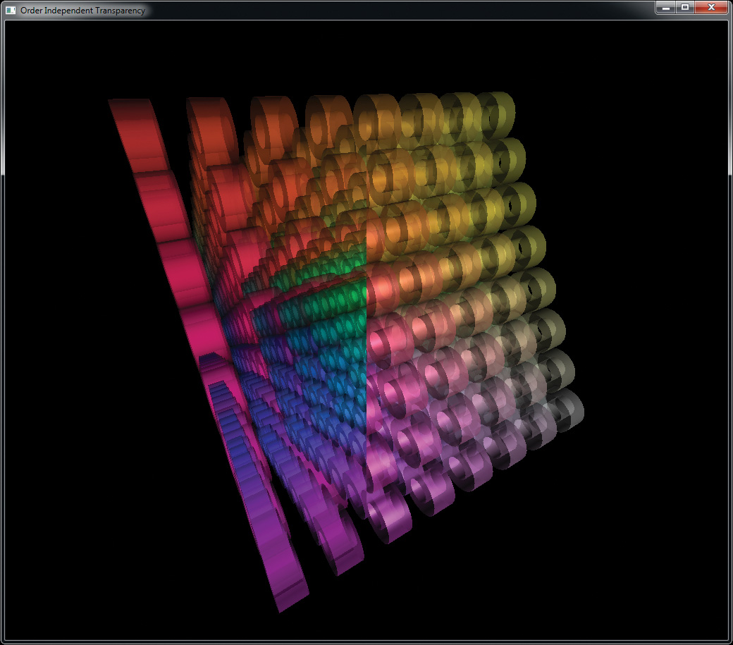
Example: Order-Independent Transparency
This section provides an example of the types of effects and techniques that can be implemented using the functionality described in this chapter. Order-independent transparency is a technique where blending operations are carried out in a manner such that rasterization order is not important. The fixed function blending provided by OpenGL through functions such as glBlendEquation() and glBlendFunc() are fairly restrictive. They provide a small, fixed set of operations that may be performed, most of which are not commutative. That is, the order of their operations matters: blend(a, blend(b, c)) does not produce the same result as blend(blend(a, b), c). This means that geometry must be sorted into a fixed, known order before being rendered. This can be very time-consuming, especially for complex geometry, and in some cases, such as where geometry may self-intersect, it may be impossible. The implementation in this example is based on a technique devised by demo engineers at AMD that uses sorted fragment lists to reorder fragments after rasterization and then perform blending in the fragment shader. This provides two benefits. First, the order in which the geometry is submitted to the GPU is not important and can be rasterized in any order. Second, arbitrary blending functions can be implemented as all operations are performed in the shader, so programmable blending is achievable.
Principles of Operation
The order-independent transparency technique described here uses OpenGL to rasterize transparent polygons. However, rather than rendering directly to the framebuffer, the fragment shader builds a set of linked lists into a large, one-dimensional buffer image. Each element in the list is a record of a fragment that contributes to the final pixel color and includes the fragment’s color, alpha, and (perhaps most important) depth. Also included in each record is the classic next pointer10 seen in almost any linked-list implementation. An atomic counter is used to keep track of the total number of fragments appended to the list so far. Each pixel on the screen generates a separate linked list of all of the transparent fragments that contribute to it. Although the fragments for all pixels are contained in the same buffer image, the resulting linked lists are interleaved, and each pixel has its own head pointer, stored in a 2D image that is the size of the framebuffer. The head pointer is updated using atomic operations. Items are always appended at the head of the image, and use of an atomic exchange operation ensures that multiple shader invocations attempting to append to the same list will not corrupt each other’s results.
10. Note that when the term pointer is used here, it is not used to refer to a physical (or virtual) address, but to an offset into the fragment buffer.
A simplified diagram of the data structures used by this algorithm is shown in Figure 11.6. Each element in the linked list is represented by a uvec4 vector and the fields used for different purposes. As uvec4 is a native type in GLSL and the OpenGL API, no special handling is required to interpret it as a structure.

In Figure 11.6, the first field (.x) of each record is used to store the next pointer (the index of the next item in the linked list). The second field (.y) is used to store the color of the fragment. It is stored in a single uint component by packing the red, green, blue, and alpha channels together in the shader, as will be shown shortly. The third component (.z) is used to store the depth of the fragment that will later be used to sort the list. As depth is a floating-point value, but we’re using integer components here, we’ll cast the floating-point value to an unsigned integer and store its bit-wise representation in the vector directly. This is a completely reversible operation and will provide the exact depth value during the sorting stage. The final component (.w) is not used currently but will be used during an enhancement to the algorithm shown later.
Once the linked list data structures have been built, a second pass is performed over the entire framebuffer. In this pass, the fragment shader traverses the linked list corresponding to its pixel and sorts all of the fragments in the list in order of depth. Once the fragments are in depth order, they can be blended together from back to front using any desired function.
To summarize, what is required for this algorithm to function are
• A buffer large enough to hold all of the fragments that might be rasterized
• An atomic counter to serve as an allocator for records within the linked list
• A 2D image the size of the framebuffer that will be used to store the head pointer for each pixel’s linked list of fragments
Initialization
Before any rendering can occur, we need to create the resources that our algorithm will use and initialize them to known values. In particular, we need to create our atomic counter that will be used to allocate items from our buffer object to store our linked list, create a 2D image the size of the framebuffer, and create a one-dimensional buffer object that is large enough to store all of the transparent fragments. Note that this doesn’t have to be large enough to store the number of pixels on the screen times the maximum expected overdraw, as most pixels will have no visible transparent fragments or perhaps very few transparent fragments. The code shown in Example 11.24 creates the required resources but does not initialize them because they need to be initialized before each frame anyway.
Example 11.24 Initializing for Order-Independent Transparency
// This is the maximum supported framebuffer width and height. We
// could support higher resolutions, but this is reasonable for
// this application
#define MAX_FRAMEBUFFER_WIDTH 2048
#define MAX_FRAMEBUFFER_HEIGHT 2048
// Local variables
GLuint * data;
size_t total_pixels = MAX_FRAMEBUFFER_WIDTH *
MAX_FRAMEBUFFER_HEIGHT;
// Create the 2D image that will be used to store the head pointers
// for the per-pixel linked lists.
GLuint head_pointer_texture;
glGenTextures(1, &head_pointer_texture);
glBindTexture(GL_TEXTURE_2D, head_pointer_texture);
glTexImage2D(GL_TEXTURE_2D, 0, // 2D texture, level 0
GL_R32UI, // 32-bit GLuint per texel
MAX_FRAMEBUFFER_WIDTH, // Width
MAX_FRAMEBUFFER_HEIGHT, // Height
0, // No border
GL_RED_INTEGER, // Single-channel
GL_UNSIGNED_INT, // Unsigned int
NULL); // No data... yet
// We will need to reinitialize the head pointer each frame. The
// easiest way to do this is probably to copy from a PBO. We'll
// create that here...
GLuint head_pointer_initializer;
glGenBuffers(1, &head_pointer_initializer);
glBindBuffer(GL_PIXEL_UNPACK_BUFFER, head_pointer_initializer);
glBufferData(GL_PIXEL_UNPACK_BUFFER,
total_pixels *
sizeof(GLuint), // 1 uint per pixel
NULL, // No data - we'll map it
GL_STATIC_DRAW); // Never going to change
data = (GLuint)glMapBuffer(GL_PIXEL_UNPACK_BUFFER, GL_WRITE_ONLY);
// 0xFF will be our 'end of list' marker.
memset(data, 0xFF, total_pixels * sizeof(GLuint));
glUnmapBuffer(GL_PIXEL_UNPACK_BUFFER);
// Next, create our atomic counter buffer to back our atomic
// counter. We need only one counter, so a small buffer will
// suffice.
GLuint atomic_counter_buffer;
glGenBuffers(1, &atomic_counter_buffer);
glBindBuffer(GL_ATOMIC_COUNTER_BUFFER, atomic_counter_buffer);
glBufferData(GL_ATOMIC_COUNTER_BUFFER, // Allocate buffer...
sizeof(GLuint), NULL, // with space for 1 GLuint
GL_DYNAMIC_COPY); // written to by GPU
// Finally, our large, one-dimensional buffer for fragment storage.
// We're going to allocate enough storage for 2 fragments for every
// pixel on the screen. Note again that this is average overdraw and
// should be sufficient and allow a few pixels to include ten's of
// fragments so long as the average remains low.
GLuint fragment_storage_buffer;
glGenBuffers(1, &fragment_storage_buffer);
glBindBuffer(GL_TEXTURE_BUFFER, fragment_storage_buffer);
glBufferData(GL_TEXTURE_BUFFER,
2 * total_pixels * // Twice the maximum number of pixels
sizeof(vec4), // Times vec4
NULL, // No data
GL_DYNAMIC_COPY); // Updated often by GPU
Rendering
For each frame, we will render the transparent objects in the scene using a fragment shader that determines the color and opacity for each fragment and then appends that information, along with the fragment’s depth, into the linked list data structures. Before each frame’s transparent objects are drawn, the head pointer and atomic counter buffers must be initialized to known values; otherwise, our shader will continue to append to the structures created in the previous frame. The code for this is given in Example 11.25.
Example 11.25 Per-Frame Reset for Order-Independent Transparency
// First, clear the head-pointer 2D image with known values. Bind it
// to the GL_TEXTURE_2D target and then initialize it from a PBO that
// has been preloaded with the value 0x00
glBindBuffer(GL_PIXEL_UNPACK_BUFFER, head_pointer_initializer);
glBindTexture(GL_TEXTURE_2D, head_pointer_texture);
glTexImage2D(GL_TEXTURE_2D, 0, // 2D texture, first level
GL_R32UI, // 32-bit GLuint per texel
MAX_FRAMEBUFFER_WIDTH, // Width
MAX_FRAMEBUFFER_HEIGHT, // Height
0, // No border
GL_UNSIGNED_INT, // Unsigned int
NULL); // Consume data from PBO
// Now bind it to the image unit that will be used for
// read-write access
glBindImageTexture(0, // Image unit 0
head_pointer_texture,
GL_FALSE, 0, // Not layered
GL_READ_WRITE, // Read and write access
GL_R32UI); // 32-bit GLuint per pixel
// Now bind the atomic counter buffer ready for use and reset the
// counter to zero
glBindBufferBase(GL_ATOMIC_COUNTER_BUFFER, // Atomic counter...
0, // Binding point 0
atomic_counter_buffer);
// Note that this also binds the buffer to the generic buffer
// binding point, so we can use that to initialize the buffer.
const GLuint zero = 0;
glBufferSubData(GL_ATOMIC_COUNTER_BUFFER, 0, sizeof(zero), &zero);
Once the code in Example 11.25 has executed, the head pointer image contains the value 0x00 in all texels and the buffer that stores our atomic counter contains zero, which resets the atomic counter to zero. Note that it is not necessary to clear the one-dimensional buffer that is used to store the linked lists, as these lists will be completely rebuilt during each frame.
Now we are ready to render the frame. First, we render all nontransparent objects, as there is no reason to append their fragments into the per-pixel fragment lists. Next, we render all of the transparent objects in an arbitrary order (this is the point of the algorithm, after all). The transparent objects are rendered using the fragment shader shown in Example 11.26.
Example 11.26 Appending Fragments to Linked List for Later Sorting
#version 420 core
// Turn on early fragment testing
layout (early_fragment_tests) in;
// This is the atomic counter used to allocate items in the
// linked list
layout (binding = 0, offset = 0) uniform atomic_uint index_counter;
// Linked list 1D buffer
layout (binding = 0, rgba32ui) uniform imageBuffer list_buffer;
// Head pointer 2D buffer
layout (binding = 1, r32ui) uniform imageRect head_pointer_image;
void main(void)
{
// First, shade the fragment -- how is not important right now.
vec4 frag_color = shadeFragment();
// Allocate an index in the linked list buffer. Remember,
// atomicCounterIncrement increments the atomic counter and
// returns the _old_ value of the counter. Thus, the first
// fragment to execute this code will receive the value 0, the
// next will receive 1, and so on.
uint new = atomicCounterIncrement(index_counter);
// Now insert the fragment into the list. To do this, we
// atomically exchange our newly allocated index with the
// current content of the head pointer image. Remember,
// imageAtomicExchange writes our new value to memory and
// returns the _old_ value.
uint old_head = imageAtomicExchange(head_pointer_image,
ivec2(gl_FragCoord.xy),
index);
// Before this code executed, we had:
// head_pointer_image(x,y) -> old_item
// Now we have
// head_pointer_image(x,y) -> new_item
// _and_
// old_head -> old_item
// Now assemble the fragment into the buffer.
// This will be the item...
uvec4 item;
// item.x = next pointer
item.x = old_head;
// Now we have
// head_pointer_image(x,y) -> new_item (.x) -> old_item.
// item.y = color
item.y = packUnorm4x8(frag_color);
// item.z = depth (gl_FragCoord.z)
item.z = floatBitsToUint(gl_FragCoord.z);
// item.w = unused (so far...)
item.w = 0;
// Write the data into the buffer at the right location
imageStore(list_buffer, index, item);
}
The shader shown in Example 11.26 appends fragments into the per-pixel linked list using atomics counters, general purpose atomic operations, bit packing, and bit casting. First, the global atomic counter is incremented in order to allocate a record in the one-dimensional linked-list buffer. This can be used as an allocator because the atomic increment operation doesn’t necessarily return (n + 1), but a new, unique value that is greater than(n). This is shown in Figure 11.7 (a). In Figure 11.7 (a), the head pointer contains the index of the first item in the linked list, and the index of the newly allocated item is stored in the new variable.

Next, this value is inserted into the head pointer texture, and the previous value of head is retrieved. This is performed in a single step by using an atomic exchange operation. This is shown in Figure 11.7 (b), where the head of the list is now pointing at the newly allocated item, and old_head contains the previous value of the head pointer—the index of the first item in the list. At this stage, the list is actually broken, as the head pointer indexes an item without a valid next pointer. However, this doesn’t matter because the list is never traversed as it is built.
Finally, the old value of the head pointer is used as the new next value for the inserted item. This means that the head pointer now refers to the item we allocated using the atomic counter, and the next pointer for that item points to what was previously the first item in the list. This is achieved by simply writing the old value of the head pointer into the next field of the new item, as shown in Figure 11.7 (c). In all parts of Figure 11.7, the new item is marked with a gray crosshatch pattern.
The result is set of unsorted lists of fragment records, each containing a color, depth, and link to the next item in the list, with one list per pixel. Notice that all of the data that might be shared between shader invocations, the atomic counter, and the head pointer is only ever modified by using atomic operations. We never actually traversed the linked list during building, as we only added items to the head. We are now ready to consume this data by sorting the fragments in order of depth and blending them together to form the final fragment color.
Finally, notice that the shader in Example 11.26 turns on early fragment testing using the early_fragment_tests layout qualifier. This is because we wish to ensure that fragments that are obscured by previously rendered opaque geometry are not added to the linked lists. As the transparent geometry is rendered with depth testing on, but the shader has side effects (writing into the linked list), OpenGL would normally perform the depth test after it has executed by default. Using the early_fragment_tests input layout qualifier instructs OpenGL to perform depth testing before the shader runs and to not execute it if the fragment fails the test. This ensures that the shader will not be executed for obscured fragments and that those fragments will not be added to the lists.
Sorting and Blending
Once the data structures have been built, the per-pixel linked lists are essentially a compressed representation of the scene. The next step is to walk the per-pixel lists and blend all of the fragments together in order to build the final output colors. To do this, we render a full-screen quad using a fragment shader that will read from the list corresponding to its output pixel, sort all of the fragments into order, and then perform the blending operations of our choice. Because the number of fragments per-pixel is expected to be low, a simple sorting algorithm can be used.
In this pass, we again take our head pointer image and our linked-list buffer and access them from the shader. However, as we are only going to be reading from them, we can bind them as a regular 2D texture and as a texture buffer object (TBO), respectively. This gives additional hints to the implementation that it can access the image in a read-only manner without worrying about coherency or caching issues. The atomic counter used to allocate list items is not required in the blending pass, as we are not going to allocate more items on the list. The main body of the sorting and blending shader is shown in Example 11.27.
Example 11.27 Main Body of Final Order-Independent Sorting Fragment Shader
#version 420 core
// Head pointer 2D buffer
uniform sampler2D head_pointer_image;
// Linked list 1D buffer
uniform samplerBuffer list_buffer;
#define MAX_FRAGMENTS 15
// Small buffer to hold all of the fragments corresponding
// to this pixel
uvec4 fragments[MAX_FRAGMENTS];
layout (location = 0) out vec4 output_color;
void main(void)
{
int frag_count;
// Traverse the list and build an array of fragments
frag_count = build_local_fragment_list();
// Sort the array in depth order
sort_fragment_list(frag_count);
// Blend the sorted fragments together to compute the final
// output color
output_color = calculate_final_color(frag_count);
}
Example 11.27 makes use of three functions. First, build_local_fragment_list traverses the linked list of fragments corresponding to the current pixel and places all of the fragments into the fragments[] array. The code for this function is shown in Example 11.28. Notice that the size of the per-pixel fragment array is defined as 15 here, even though the buffer allocated in Example 11.24 is only twice the number of pixels in the framebuffer. This is possible because the fragment lists needs to be only large enough to store the average number of fragments per-pixel, but the maximum overdraw supported can be much larger.
Example 11.28 Traversing Linked-Lists in a Fragment Shader
// Traverse the linked list, place all of the fragments into the
// fragments[] array, and return the number of fragments retrieved
// from the list.
int build_local_fragment_list(void)
{
uint current;
int frag_count = 0;
// Get the initial head pointer from the header-pointer image
current = texelFetch(head_pointer_image,
ivec2(gl_FragCoord.xy), 0);
// While we haven't reached the end of the list or exhausted the
// storage available in fragments[]...
while (current != 0xFFFFFFFF && frag_count < MAX_FRAGMENTS)
{
// Read an item from the linked list
item = texelFetch(list_buffer, current);
// item.x contains the 'next' pointer - update current
current = item.x;
// Store the fragment in the array
uvec4 fragments[frag_count] = item;
// Update the fragment count
frag_count++;
}
// Done - return the fragment count
return frag_count;
}
After the local array of fragments has been built, it is sorted in order of depth using the sort_fragment_list function shown in Example 11.29. This function implements a simple bubble-sort algorithm. While this is a simple algorithm and is not well suited for sorting large amounts of data because the number of items is very low, the cost of the function is still small, and the algorithm suffices.
Example 11.29 Sorting Fragments into Depth Order for OIT
// Simple bubble-sort for sorting the fragments[] array
void sort_fragment_list(int frag_count)
{
int i;
int j;
for (i = 0; i < frag_count; i++)
{
for (j = i + 1; j < frag_count; j++)
{
// The depth of each fragment is bit-encoded into the
// .z channel of the fragment array. Unpack it here.
float depth_i = uintBitsToFloat(fragments[i].z);
float depth_j = uintBitsToFloat(fragments[j].z);
// Compare depth and if the comparison fails...
if (depth_i > depth_j)
{
// Swap the fragments in the array
uvec4 temp = fragments[i];
fragments[i] = fragments[j];
fragments[j] = temp;
}
}
}
}
One the fragments in the fragments[] array have been sorted into depth order, we can traverse the array and blend the fragments together using a blending operation of our choice. This is implemented in the calculate_final_color function, which is shown in Example 11.30.
Example 11.30 Blending Sorted Fragments for OIT
// Simple alpha blending function -- we could replace this with
// anything...
vec4 blend(vec4 current_color, vec4 new_color)
{
return mix(current_color, new_color, new_color.a);
}
// Function for calculating the final output color. Walks the
// fragments[] array and blends each pixel on top of each other
vec4 calculate_final_color(int frag_count)
{
// Initialize the final color output
vec4 final_color = vec4(0.0);
// For each fragment in the array...
for (i = 0; i < frag_count; i++)
{
// The color is stored packed into the .y channel of the
// fragment vector. Unpack it here.
vec4 frag_color = unpackUnorm4x8(fragments[i].y);
// Now call the blending function.
final_color = blend(final_color, frag_color);
}
// Done -- return the final color.
return final_color;
}
The blend function shown in Example 11.30 simply uses the mix function to implement basic alpha blending. This is equivalent to using fixed-function OpenGL blending with the blend equation set to GL_FUNC_ADD and the blend functions set to GL_SRC_ALPHA and GL_ONE_MINUS_SRC_ALPHA for source and destination factors, respectively.
Results
The results of rendering with this algorithm are shown in Figure 11.8. The image on the left is produced using fixed-function OpenGL blending. As can be seen, the image does not look correct in all areas. This is because geometry is rendered in order of submission rather than in order of depth. Because the blending equations used are not commutative and are therefore sensitive to order, they produce different results depending on the submission order of the geometry. Contrast this to the result shown on the right of Figure 11.8. This is rendered with the order-independent algorithm described in this example. The result is correct in all areas.