Chapter 11. Extensional Structures: Balancing and Interpretation*
* For all figures in this chapter (in the printed book only), see the preface for information about registering your copy on the InformIT site for access to the electronic versions in color.
Introduction
In the first edition of this text, we mentioned that the balancing of extensional structures was in the initial stages of development. Since then, several major oil companies have successfully applied extensional balancing concepts in the northern Gulf of Mexico, Nigeria, Indonesia, Brazil, and elsewhere (Dula 1991; Nunns 1991; Withjack et al. 1995; Shaw et al. 1997; Shaw et al. 2005). Accordingly, we now have a higher degree of confidence in extensional structural and balancing methods and techniques. As with compressional structural geology and balancing, a common theme to this chapter is the relationship between hanging wall fold geometry and fault geometry. Thus, we introduce a new method in the section Using Structural Relief and Throw to Predict Downthrown Stratigraphic Section. In this section, we describe how to project footwall sand and its associated downthrown depth into the hanging wall. Similarly, in shale units, footwall porosity or hydrocarbon content information can also be projected downthrown into the corresponding hanging wall correlations. The method has high square correlations and is based on closed form solutions to the extensional balancing problem.
This chapter is divided into two parts. The first is the origin of hanging wall anticlines (commonly called rollover anticlines or rollovers), antithetic and synthetic faults, and keystone structures, and how knowledge of the genesis of a structure can help find additional hydrocarbons (Tearpock et al. 1994). We address such subjects as (1) why some growth faults die in both the upward and downward directions and what this means to exploration, (2) where rollover anticlines are likely to exist or be positioned along major listric normal faults (i.e., faults that exhibit large vertical expansion across the fault surface), and (3) how faults form prospects. The second part of the chapter is the study of compaction effects along growth normal faults and how sandstone/shale ratios are utilized to project growth faults into poor data areas or, conversely, how fault shape is used to predict percent sand in the footwall of the fault. The chapter ends with projecting footwall correlations into the corresponding downthrown and undrilled hanging wall section.
Origin of Hanging Wall (Rollover) Anticlines
Often, geoscientists work on the edge of coherent data or in areas where seismic data deteriorates. In this section, we present methods for extrapolating known data into poor data areas. Rollover anticlines have been successfully drilled for many years, yet questions remain concerning their origin and how rollovers form prospects. A major insight into the origin of rollover was initiated by Hamblin (1965) when he recognized that these strange “reverse drag folds” are the natural consequence of motion along listric normal faults. He reasoned that if the hanging wall block separates from the footwall block, a small void opens between the two blocks. Collapse due to gravity would instantaneously close the void and, as the hanging wall block collapses onto the footwall block, a reverse drag structure forms. However, Hamblin did not exactly specify how this gravitational collapse occurs. Gibbs (1984) later recognized from North Sea data that extensional structures (as an analogy with compressional structures) seemed to form duplexes, complete with horses, transfer zones, and so on. Yet a number of questions remain to be fully answered, such as:
Can the shallow portion of rollover structures be used (a) to predict the deeper structure (e.g., subfault structure) or (b) to extrapolate into regions of poor or nonexistent data (e.g., into poorly imaged seismic zones)?
What is the precise origin of rollover structures, and is it possible to predict the amplitude, style, and position of a rollover from observable and mappable geologic features?
What are the origins of the antithetic, or compensating, faults and the keystone structures, and how do these structures influence rollover geometry?
What causes some (perhaps most) antithetic growth faults to exhibit displacements along their surfaces that die in both the upward and downward directions in a seemingly contradictory relationship?
Answers to at least some of these questions should aid geoscientists in reducing the time and expense in (1) locating rollovers; (2) generating better interpretations, maps, and prospects; and (3) isolating trapping mechanisms. Our studies and those of others suggest that compaction, fault shape, antithetic and synthetic faulting, and cross structures affect the geometry of rollover structures.
When developing a theory for a structure that is as complex as a rollover, the initial theories are likely to be overly simplistic (Eichelberger et al. 2017). Our position is that a theory is only as good as its ability to quantitatively explain the observations. Therefore, and although less work has been conducted on extensional balancing in recent years, we expect that in the future, modifications and refinements are likely to make these theories more exacting.
Coulomb Collapse Theory
A theory of rollover formation based on Coulomb failure, or breakup (Suppe 1985) of the hanging wall onto the footwall block, has been advanced by Xiao and Suppe (1988, 1992), Groshong (1989), and others. According to this theory, rocks fail along Coulomb fracture surfaces oriented at about 20 deg to 30 deg to the maximum principal stress (σ1) (Billings 1972), which in the case of extensional deformation is subvertical. This theory describes many of the features observed on seismic sections, and the model commonly mimics observed rollover geometries subject to depth correction (Fig. 11-1). An understanding of this theory of genesis of rollovers can help you better interpret rollover geometries in poor data areas and thereby generate better prospects (Tearpock et al. 1994).

Figure 11-1 Comparison of (a) Brazos Ridge seismic data to (b) computer model, utilizing the Coulomb breakup theory. (Published by permission of H. Xiao and J. Suppe.)
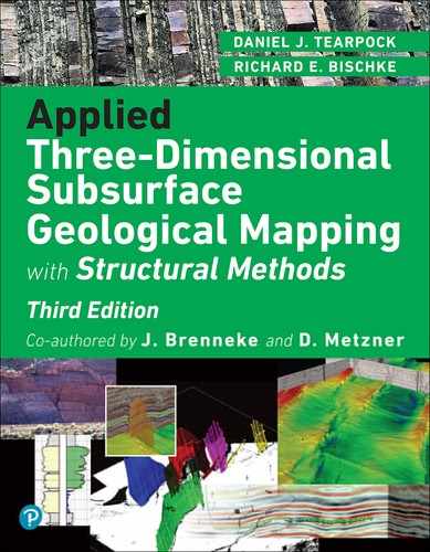
The elements of the Coulomb theory are shown in Figure 11-2a through e. Figure 11-2 represents the initial prefaulted or pregrowth state. This simple example shows an incipient major fault that has, for purposes of demonstration, a single concave upward bend. In nature, major listric normal faults are normally curved, and this more realistic case can be duplicated by introducing several concave upward bends into a model.
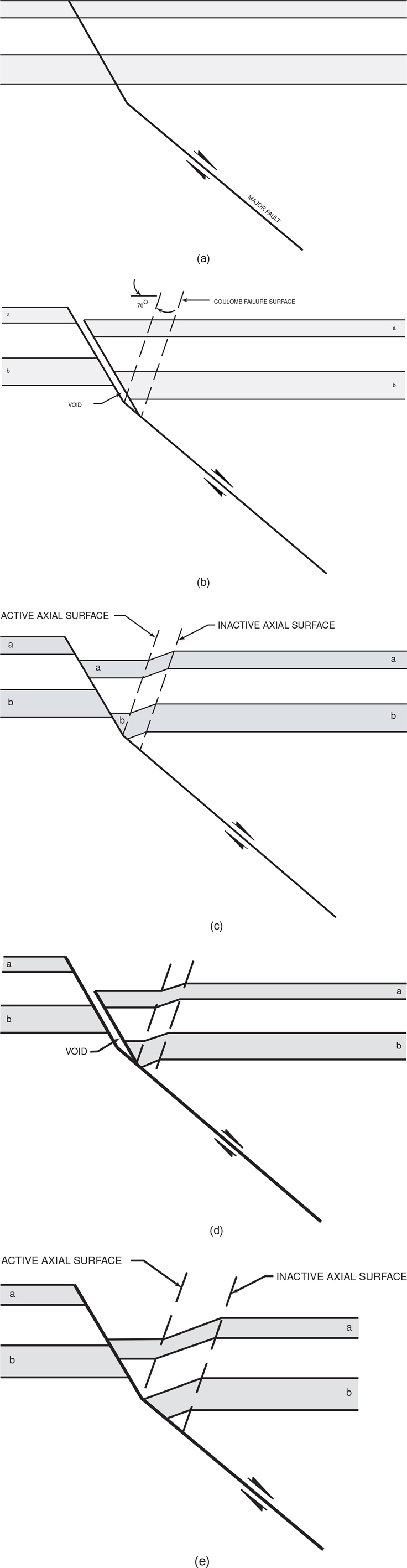
Figure 11-2 (a)–(e) Coulomb failure or shear collapse model showing different stages in the development of a simple rollover. A bend in the major fault subjects the hanging wall to deformation at the active axial surface, which is fixed to the bend in the footwall. Increased slip causes the inactive axial surface to migrate away from the surface of active deformation. (Modified after Suppe 1988. Published by permission of John Suppe.)
As the hanging wall block moves over the footwall block, a small void opens between the hanging wall and the footwall blocks, as described by Hamblin (1965) (Fig. 11-2b). Gravitational forces cause the hanging wall block to instantaneously collapse into the hole (created by the sliding) along the Coulomb failure surfaces. In Figure 11-2b the Coulomb collapse angle is 70 deg with respect to the horizontal. Beds in the hanging wall shear parallel to the Coulomb failure surfaces, and the material fills the hole, causing the beds to extend (Fig. 11-2c).
Observe in Figure 11-2b and c that material experiences rotation as it passes through the Coulomb shear surface that is fixed to the concave upward bend in the major fault. This is a locus of deformation that extends upward through the strata and, for that reason, this shear surface is called an active axial surface (Fig. 11-2c). Deformation occurs only along active axial surfaces, which are affixed to the bends in listric faults.
Initially, the material that passes through the bend in the normal fault is deformed at the active axial surface and is translated basinward. This material lies adjacent to the inactive axial surface, basinward of which the strata are undeformed (Fig. 11-2c). The inactive axial surface rides passively along the straight portion of the fault surface as movement progresses. As this surface is not affixed to the bend in the fault surface that creates the void, the inactive surface is passive and does not cause the hanging wall beds to dip toward the fault surface. Notice that the slip on the fault surface is the distance between the active and inactive fault surfaces, parallel to the fault surface.
This process is more readily understood if the fault model is subject to another increment of sliding (Fig. 11-2d). Of course, in nature these increments are infinitesimal. The sliding opens another void between the hanging wall and the footwall blocks, and the active axial surface that formed in Figure 11-2c translates basinward (Fig. 11-2d). However, the void instantaneously closes by gravitational shear failure, pinning the active axial surface to the bend. The resultant structure shown in Figure 11-2e contains a graben-like feature adjacent to the steepest portion of the major fault and is a monoclinally shaped rollover structure. Sedimentary compaction within the basin creates basinward dip and closes the structure in the direction to the right in the figure.
You can better understand these processes by redrawing Figure 11-2e and cutting the hanging wall block from the footwall block with scissors. Then subject the major fault to another increment of motion and collapse the suspended material onto the footwall parallel to the Coulomb failure surfaces.
Growth Sedimentation
In areas like the Gulf of Mexico, most major normal faults are active growth faults. This means that sedimentation occurs simultaneously with fault slip, and thus the stratigraphic intervals are subject to vertical expansion across the fault surface (i.e., the intervals thicken on the downthrown side of the growth fault). How does this syndepositional sedimentation affect the structure, and can an analysis of this growth aid us in finding hydrocarbons?
Referring back to Figure 11-2c, let us assume that a layer of sediment is deposited across the hanging wall and footwall portions of our structure (Fig. 11-3a). The graben-like feature contains more accommodation space than the top of the rollover, so the sediments will be thickest over the graben and thinner over the footwall and the crestal portions of the monoclinal rollover. We saw in Figure 11-2b through e that the active axial surface is fixed to the bend in the major fault and that it represents the locus of deformation of the hanging wall beds. The inactive axial surface is passive and migrates basinward. Notice in Figure 11-3a that the inactive surface does not extend upward into the recently deposited growth sediments. The active axial surface, however, is a locus of active deformation that affects the entire body of growth sediments. When deformation is viewed as an incremental process, a growth axial surface must connect the active axial surface to the inactive axial surface, as shown in Figure 11-3a. You can convince yourself of this statement by visualizing a thin layer of additional growth sediments deposited above layer 1. This layer will be horizontal. Another small increment of sliding along the major fault causes Coulomb collapse that deforms this recently deposited layer in the region where the active and the growth axial surfaces converge (Fig. 11-3a). An additional increment of sliding, combined with growth sedimentation, produces the geometry observed in Figure 11-3b. The growth wedge expands as the growth sediments move through the active axial surface.
Figure 11-3 (a)–(b) Rollover development showing deformation during growth sedimentation. The most recently deposited sediments are deformed at the point where the active and growth axial surfaces converge. (Modified after Suppe 1988. Published by permission of John Suppe.)
For larger rollover structures, sands are more likely to be deposited in the graben, whereas suspended sediments are more likely to be dominant across the top of the rollover. Therefore, facies changes and stratigraphic traps are predicted to occur in the vicinity of the growth axial surface. A more realistic example of growth faulting is presented in the following section on projecting large growth faults to depth.
The growth axial surface can be located on a seismic section by using dip domain analysis (Tearpock et al. 1994). This surface is located between the steeper-dipping beds at the front of the structure and the flatter-dipping beds located at the crest. After you locate the growth axial surface, you can determine the stratigraphic interval that was deposited as the structure grew. This is important, as no structure exists to trap hydrocarbons prior to the growth phase. To determine the growth phase of the structure, follow the growth axial surface downward. The growth axial surface subparallels the main fault during the time of growth, thus delimiting the history of the structural growth. The growth axial surface terminates at the inactive axial surface, and this point indicates the top of the pregrowth strata (Fig. 11-3a and b). No structure existed during the pregrowth phase of sedimentation to trap hydrocarbons (Fig. 11-2a).
Example of a Rollover Structure.
Some listric faults are observed to dip more gently with depth and then, at greater depth, to increase in dip (Fig. 11-12). This creates a concave downward bend in the major fault. Above this bend, the Coulomb collapse theory predicts that the deformation takes place along basinward-dipping conjugate shear surfaces. Shear can occur along two conjugate surfaces (Billings 1972) and, in our example, this shear occurs in the clockwise direction (Fig. 11-4a).

Figure 11-4 Deformation of growth sediments at the bends in normal faults. (a) A downward bend in the fault activates basinward dipping or synthetic shear. (b) An upward bend activates landward or antithetic shear. (c) Simple generic model of Brazos Ridge rollover development, not including compaction. (Published by permission of H. Xiao and J. Suppe.)
The Brazos Ridge, in the northern Gulf of Mexico, can be used to demonstrate the Coulomb breakup theory for a more realistic case. The Corsair fault is the major listric normal fault in the Brazos Ridge area. In the most general sense, the Corsair fault dips at about 45 deg, flattens to about 10 deg, and then steepens to approximately 20 deg, as represented in a computer model in Figure 11-4c. The Brazos region is subject to synchronous deformation and sedimentation, and thus the sediments deposited in the hanging wall block are growth sediments. If the simple Corsair fault model described in Figure 11-4c were subject to gravitational (basinward) sliding, two voids would be created, one above the concave-up portion and the other adjacent to the concave-down portion of the master fault. Clockwise collapse above the deeper concave downward bend (Fig. 11-4a) and counterclockwise collapse above the concave upward bend (Fig. 11-4b) would produce the geometry observed in Figure 11-4c. Notice that there is a relationship between the shape of the fault and the shape of the rollover in the hanging wall.
If deposition rates are high, as in the Brazos Ridge area, the sediments will fill the low area adjacent to the shallowest portions of the major fault, thin over the top of the rollover structure, and then thicken basinward (Fig. 11-4c). The vertical expansion of stratigraphic intervals, as observed in this example, demonstrates why the sediments are referred to as growth sediments. Also notice the growth axial surface in Figure 11-4c. It subparallels the growth fault, and it terminates with depth at an inactive axial surface that dips toward the fault (compare to Fig. 11-3b). The model in Figure 11-4c contains rollover amplitudes that are higher than observed along the Brazos Ridge (Fig. 11-1a). However, compaction combined with synthetic and antithetic crestal faulting reduces the amplitudes of rollovers.
The thickness of the crestal growth section can vary with the shape of the fault. In the case of the Brazos Ridge, the large expansion fault that creates the structure dips at about a 20-deg angle at depth. Thus, as the hanging wall moves over the footwall, the hanging wall slides down a 20-deg dipping fault surface. This slope causes the hanging wall to drop in elevation relative to the footwall, and the downward motion creates ample space for the accumulation of thick growth section over the crest of the structure (Figs. 11-3a and 11-12). Later we show that this fault geometry creates productive four-way closures (Fig. 11-21).
However, if a large expansion fault flattens at depth and is subhorizontal, then as the hanging wall moves over the footwall, the crest of the rollover structure does not change elevation with respect to the footwall (Fig. 11-5). This fault geometry creates the classic half-graben structure, with accommodation space developing between the fault and the flank of the half-graben structure but not over the crest of the structure. In this case the growth sediments are more likely to thin onto the flank of structure, creating stratigraphic traps. However, on actively growing structures, this thinning results from an interaction of stratigraphic and structural processes, classified under the heading of tectonostratigraphy (Chapter 13). Figure 11-5 shows a seismic profile of a half-graben structure from the Central Sumatra Basin, Indonesia. As the structure grows, growth sediments deposited in the half-graben structural low will be subject to axial surface deformation, as shown in Figure 11-5. The growth sedimentary section thins dramatically across the growth axial surfaces and onto the flank of structure (Suppe et al. 1992; Shaw et al. 1997). As growth sedimentation is typically episodic, alternating between high and low sedimentation rates, the local subsidence rate resulting from fault motion may temporarily exceed the sedimentation rate. In this case, coarser sediments may fill the accommodation space in the half-graben (Xiao and Suppe 1992). As the sedimentation versus subsidence rates fluctuate, the tectonostratigraphic process creates facies changes and unconformities along strike and down-dip of the growth axial surfaces.
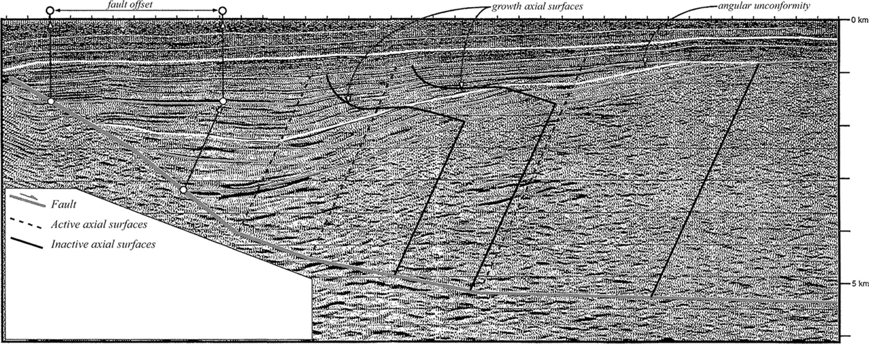
Figure 11-5 Seismic profile of a half-graben structure from Central Sumatra Basin, Indonesia, showing axial surfaces emanating from bends in the fault surface. Growth axial surfaces on the flank of the structure (subhorizontal curved lines) define the position where growth section thins onto structure. The syntectonic sedimentation created potential facies changes and unconformities at the position of growth axial surfaces. (From Shaw et al. 1997. AAPG©1997, reprinted by permission of the AAPG whose permission is required for further use.)
Provided that information exists on the shape of a fault that has created a rollover, the Coulomb breakup theory can be used to predict the rollover angle (θ) or bed dips. Based on Coulomb deformation, the rollover angle (θ) is related to the change in fault dip (f) through a complicated set of trigonometric formulae, which can be represented by graphs (Fig. 11-6a and b). The assumptions used in the graphs are that the material in the hanging wall is subject to Coulomb collapse and that the structure has not experienced sedimentary compaction, as described later in this chapter in the section Compaction Effects along Growth Normal Faults. Thus, these diagrams strictly apply to the nongrowth phase of the sedimentation and will approximate the rollover angle within growth sediments. Let us assume that a seismic section images the shallow and deeper portions of a listric fault but does not image the bed dips. If the above conditions are met and if the initial fault dip (β) and the fault dip at a deeper level (α1) can be observed on a depth-converted seismic section, then the rollover dip can be estimated from Figure 11-6a or b. Figure 11-6a assumes a Coulomb breakup angle of 60 deg, whereas Figure 11-6b assumes a 70-deg breakup angle. For example, the Brazos Ridge generally has a major fault that initially dips at about 45 deg and flattens abruptly to about 15 deg. Therefore, the change in fault dip f= 30 deg. From Figure 11-6a and b, the predicted bed dips at the front of the rollover structures are estimated to be 18 deg to 22 deg. Even though the Brazos Ridge growth sediments have been subject to compaction, these results compare favorably to observed bed dips, which average about 20 deg at the bend in the fault (see Fig. 11-1a and b). For presentation purposes, Figure 11-6a and b can also be used to generate generic or idealized models of real rollover structures. The generic structure shows how the rollover structure formed.
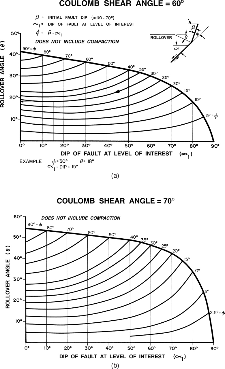
Figure 11-6 (a) Theoretical prediction of rollover angle (θ) from fault dips (ϕ and α 1) for a Coulomb shear angle of 60 deg. Diagram does not include compaction. (b) Same as (a), but for a Coulomb shear angle of 70 deg. (Published by permission of R. Bischke.)
A Graphical Dip Domain Technique for Projecting Large Growth Faults to Depth
Often, geoscientists work on the edge of, or below the level of, coherent seismic data. Large listric normal faults may be present in the poor data zone. If a proposed well crosses a large growth fault and the well encounters an unexpected stratigraphic section, the result is often disappointment and confusion regarding the geology. Also, large growth faults commonly are pressure-sealing faults, so the unexpected penetration of a large fault by a drilling well could be disastrous.
On the Gulf of Mexico shelf, in Indonesia, China, Nigeria, and elsewhere, rollover structures form downthrown to listric growth faults. Growth sequences of sediments that accumulate downthrown to normal faults are common throughout the world. We use these growth sections to formulate a technique for projecting normal faults into poor data areas using the well-imaged portions of rollover structures.
In the section on the origin of rollover, we show how rollover structures form as the hanging wall conforms to the shape of the footwall. Thus, there is a causative relationship between the shape of the fault and the shape of the fold. We use this causative relationship to present a graphical technique for projecting large growth faults into poor data areas. This inclined shear collapse technique is subject to measurement errors. Therefore, the method can project a fault through only a limited number of bends (two or three) within poor data zones. In order to compare theory to observation, we present a well-constrained example of projecting a fault surface to depth using the shallow parts of a rollover structure.
We base our graphical method on the kinematics developed by Hamblin (1965) and make no assumption as to the shape of the fault surface. For example, the fault surface can contain both concave and convex bends, and the fault surface need not flatten at depth. Bischke and Tearpock (1999) present formulas for projecting faults to depth and for calculating Coulomb collapse angles. The Coulomb collapse angle formula requires knowledge of fault throw and has application to rollover structures in extensional environments anywhere in the world. We also present a graphical method for predicting Coulomb collapse angles in this section.
Rollover Geometry Features
A major advancement in the understanding of structures occurred when Hamblin (1965) recognized that rollover anticlines form as hanging wall beds slip along listric normal faults. As the hanging wall slides along the fault surface, the hanging wall conforms to the shape of the fault surface by collapsing onto the fault surface. Hamblin indicated that the process could result from vertical or Coulomb collapse (Fig. 11-7). Numerous authors tested the two mechanisms and favor Coulomb collapse over the vertical collapse mechanism (White et al. 1986; Worrall and Snelson 1989; Groshong 1989; Bischke and Suppe 1990b; Dula 1991; Nunns 1991; Withjack et al. 1995). Xiao and Suppe (1992) show, from empirical observations using forward models, that many rollovers form as a result of Coulomb collapse at angles of 65 deg to 70 deg with respect to the horizontal. Industrial software programs are available that incorporate the vertical and inclined collapse algorithms to model rollover structures (Rowan and Kligfield 1989).
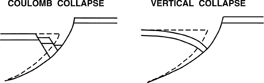
Figure 11-7 Rollovers form as the hanging wall collapses onto the footwall. Hanging wall collapse could occur as inclined (Coulomb) collapse or as vertical collapse. (Modified after Hamblin 1965. Published by permission of the Geological Society of America.)
In a listric normal fault system, as the hanging wall beds move through bends in the fault surface, small voids open between the hanging wall and the footwall (Fig. 11-7). Large gravitational forces instantaneously close these voids, forcing the hanging wall to conform to the shape of the footwall. This collapse mechanism causes the hanging wall beds to dip, or diverge, toward the fault surface (Fig. 11-8). Furthermore, the strata steepen in dip as they move across bends in the fault, so the more listric the fault surface, the steeper the dip of the beds (Fig. 11-8).
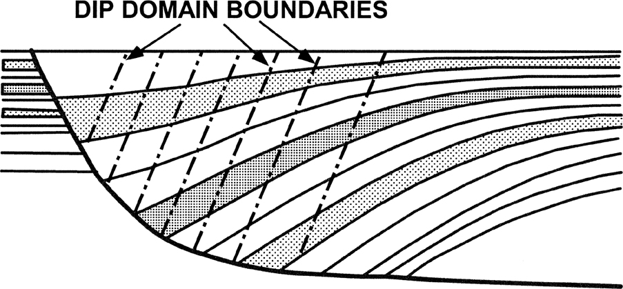
Figure 11-8 Listric normal faults cause the hanging wall beds to diverge toward the fault as the beds move through bends in fault surfaces. The fault bends define the dip domain boundaries. Young growth sediments dip at gentle angles relative to the deeper beds, as the shallow beds have not moved through many fault bends. The older and deeper beds, having moved through many fault bends, dip at higher angles. (Modified from Xiao and Suppe 1992. Published by permission of the Gulf Coast Association of Petroleum Geologists.)
Motion of the hanging wall down the fault surface creates accommodation space for growth sediments. The recently deposited sediments, having existed for only a short period of time, have not moved through many fault bends and therefore exhibit gentle bed dips (Fig. 11-8). The deeper and older sediments have moved through numerous fault bends (Xiao and Suppe 1992). Thus, older growth sediments dip at higher angles than shallow growth sediments (Fig. 11-8).
Several observations can be made about rollover fold shapes. First, the more listric the fault, the steeper the dip of the growth section. Second, there is a relationship between fault shape and rollover shape. If fault shape is known, then rollover geometry can be predicted with a high degree of certainty (Xiao and Suppe 1992; Shaw et al. 1997). Conversely, if rollover shape is known, then fault shape can be predicted, but with less certainty. Predicting fault shape from rollover shape is an inverse technique and calculation errors accumulate. These errors originate from uncertainties resulting from depth correction, geological and stratigraphic variations, and simple measurement errors. However, both techniques are important tools in extensional structural interpretation.
Projecting Large Normal Faults to Depth
We present a graphical method for projecting large normal faults to depth using hanging wall beds that have been subject to noticeable rollover. We also present methods for estimating fault shape and position from the shape of a well-constrained rollover structure.
In order to apply this method, two features must be known: (1) a marker bed that exhibits noticeable rollover and (2) the true dip of the fault at the hanging wall cutoff level of the marker beds. A profile is constructed that must be a dip profile, so that it is perpendicular (as close as possible) to strike of the fault and strike of the beds. A fault surface map can help you determine the dip direction of the profile. The structural information can come from well log data, depth-corrected seismic profiles, or cross sections. If possible, start the projection process by locating a marker bed above the known level of the main expansion fault. Then use the known portions of the fault to calibrate and test the projection procedure. If satisfied with the results, apply the method to the unknown levels of the fault.
Procedures for Projecting Large Normal Faults to Depth
If using a seismic profile, depth-correct the seismic section over the interval of concern. Depth-correct the section on the workstation using local checkshot or other more modern depth conversion methods such as employing formation tops to calibrate models derived from time surfaces and processing velocities.
If secondary faulting offsets the marker bed, restore the bed to its unfaulted position before proceeding further. This is readily done by scanning or digitizing the marker bed into a graphics program and restoring the upthrown and downthrown cutoffs of the marker bed (Bischke and Tearpock 1999).
In the graphics program, locate a deep marker bed on a level that intersects the main fault. The bed should exhibit obvious rollover and intersect the imaged portion of the main fault (Fig. 11-9a).
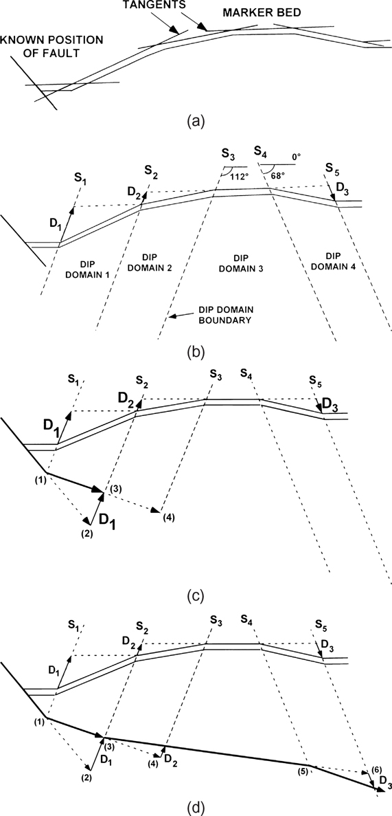
Figure 11-9 (a)–(d) Graphical procedures for projecting a normal fault to depth, using the shape of a generic rollover. For explanation, see text.
Fit tangents to the marker bed in order to segment the rollover into dip domains (see Cross-Section Construction and Kink Method Approximation sections in Chapter 10). Each dip domain contains a region of roughly uniform bed dips (Shaw et al. 1997). Curved rollovers will possess several dip domains (Figs. 11-8 and 11-9a). Our generic example has four important dip domains: dip domains 1, 2, 3, and 4 (Fig. 11-9b). Where the tangent lines intersect, construct five dip domain boundary lines (S1, S2, S3, S4, and S5) to each of the dip domain panels (Fig. 11-9b). The dip domain boundaries are drawn at an angle of either 68 deg or 112 deg. In Figure 11-9b, dip is measured clockwise, with 0 deg to the right and 180 deg to the left. If the marker bed dips toward the main fault, then these domain boundaries dip at about 112 deg with respect to the horizontal, and they dip in the antithetic direction toward the main fault. If the marker bed dips away from the main fault, then these domain boundaries dip at about 68 deg in the synthetic direction, or in the same direction as the main fault. As an alternative to the above assumed angles, you can derive the collapse angle from the geometry of rollover structures, as described later in the chapter (Bischke and Tearpock 1999).
Project the first dip domain boundary S1 downward to where it intersects the straight-line projection of the main fault surface (Fig. 11-9c). Where the two surfaces intersect at point (1), the fault dip decreases and the fault becomes more listric.
As the first step to determine the fault position beyond the first bend in the main fault, construct horizontal lines between the right and the left dip domain boundaries, or between boundaries S1 and S2, S2 and S3, and so on (Fig. 11-9b and c). Then, parallel to the dip domain boundaries and between the marker bed and the horizontal line, measure the distances D1, D2, and D3. In other words, measure distances D1 and D2 along the 112-deg inclined dip domain boundaries. Similarly, measure distance D3 along the 68-deg inclined dip domain boundary S5 (Fig. 11-9c).
Next, project the known portion of the main fault forward, from the left domain boundary at point (1) to the projection of the right dip domain boundary at point (2) (Fig. 11-9c). Where the straight-line projection of the main fault intersects the right domain boundary S2, measure the distance D1 from point (2) upward and in line with the right domain boundary S2. This procedure determines the position of point (3). The position of the main fault is now known at point (1) and at its projected position at point (3), defined by distance D1. Next, construct the projected portion of the fault surface between points (1) and (3), establishing the position of the fault beneath dip domain 1 (Fig. 11-9c).
Project the main fault forward from point (3) to point (4) (Fig. 11-9c) and repeat step 7 for the next fault bend (Fig. 11-9d). For this fault bend, measure distance D2 from point (4) at the right domain boundary S3 (Fig. 11-9d).
If the rollover has a horizontal crest, this means that the fault does not change dip beneath the flat crest of the rollover. Thus, the main fault dips at the same angle beneath the crest of the rollover (Fig. 11-9d). In other words, the fault is straight beneath dip domain 3 in Figure 11-9b. Project the fault beneath the flat crest to dip domain boundary S4 at point (5). At point (5) the fault turns down and becomes convex where the beds turn down, but what is the dip of the fault beyond dip domain boundary S4?
Repeat step 7 again, but in this case, the fault turns down at the axial surface where the marker bed turns down. So subtract distance D3 from point (6). Lastly, we construct the convex projection of the fault surface beneath dip domain 4 (Fig. 11-9d).
This technique is very precise on ideal or generic rollovers, but it suffers from measurement errors and geologic variations on real rollover structures, where these measurement errors add through each fault bend. Therefore, the projection technique may deteriorate after projecting the fault surface through three or four fault bends.
Field Example.
The method has application to all extensional regimes. A field example of a rollover structure from the Gulf of Mexico basin illustrates the procedures used to employ the fault projection method.
The example is from a 3D depth-corrected profile from the Burgentine Lake Field, onshore Texas (Fig. 11-10) (Bischke and Tearpock 1999). The horizons and fault surface were tied to well log data and mapped. The profile was depth-corrected using checkshot data. A graphical technique for determining the Coulomb collapse angle (described in the next section) derives a collapse angle ψ of 63 deg for the structure (Fig. 11-10a). This angle is slightly less than the 67-deg to 68-deg collapse angles observed on some Gulf of Mexico rollovers (Xiao and Suppe 1992). Employing the steps described in the preceding section on procedures, and using a ψ of 63 deg, we generate the cross section shown in Figure 11-10b. The projected portion of the fault surface lies over the depth-corrected portion of the fault surface. In this example, the agreement between theory and observation is very good. Therefore, we have shown that the method has application in working with real rollover structures.
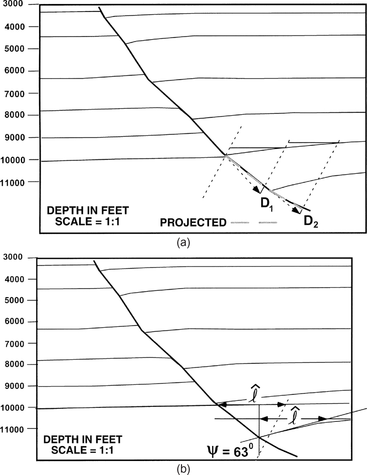
Figure 11-10 (a) Graphical procedures for determining the Coulomb collapse angle on a rollover anticline at Burgentine Lake, Texas, USA. For detailed explanations, see text. (b) Predicted fault surface conforms to depth-corrected fault surface [dashed in (a)].
Determining the Coulomb Collapse Angles from Rollover Structures
We conclude this section by describing a graphical technique for determining the Coulomb collapse angle. In Bischke and Tearpock (1999), we present the mathematical basis for these graphical methods. Here we describe the graphical method.
Using a dip-oriented, depth-corrected seismic profile, begin by locating a deep dip domain that lies adjacent to a large expansion fault, as outlined by the dashed lines in the hanging wall block in Figure 11-11a. The fault is represented by the lines L and S. A tangent line ℓ is fit to the steepest dipping beds adjacent to the fault surface, and another tangent line is fit to the flat crest of the rollover. The technique requires the determination of two displacement parameters: (1) the throw T on the fault and (2) the vertical distance V between the marker bed’s footwall position and the position of the marker bed at the crest of the rollover (Fig. 11-11b).
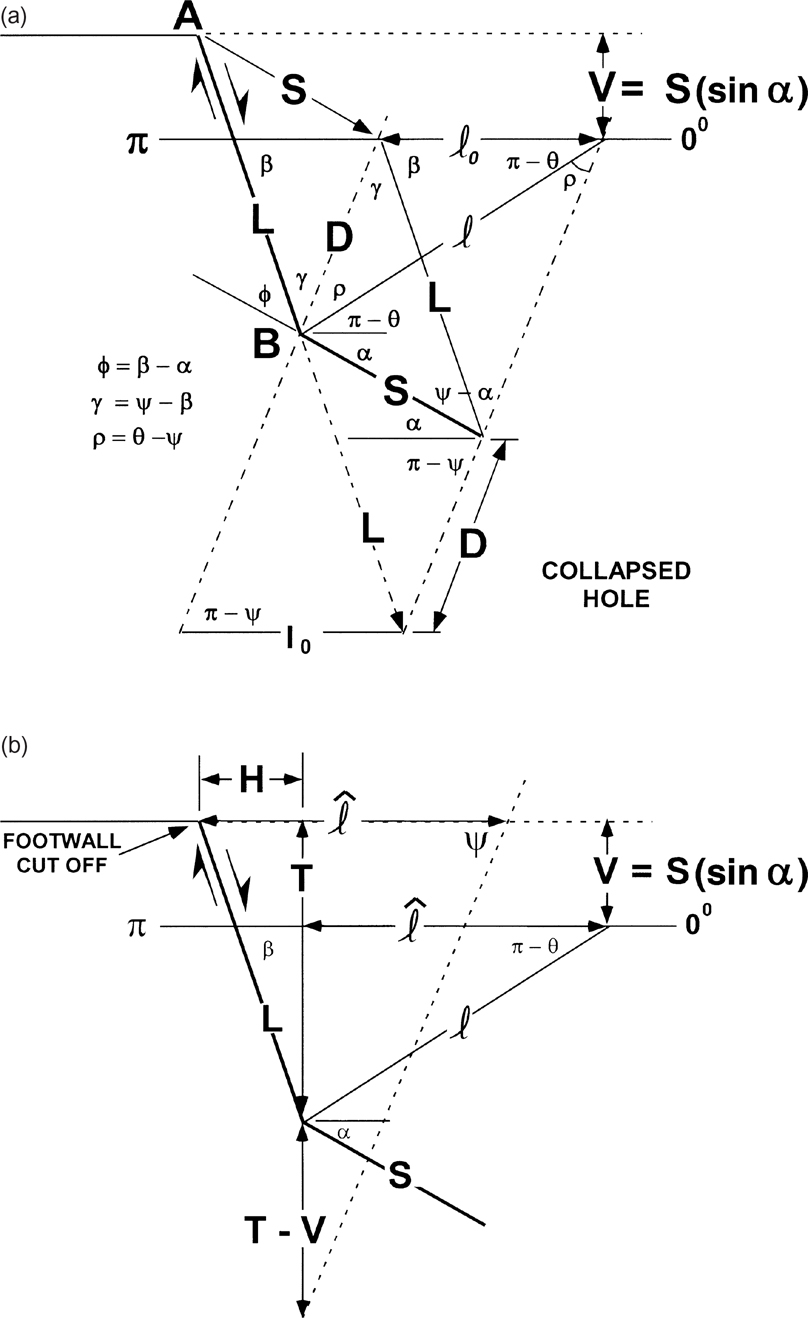
Figure 11-11 (a)–(b) Graphical method for predicting Coulomb collapse angles from rollover structures. For detailed explanations, see text.
At the position of the marker bed’s hanging wall cutoff, construct the vertical throw vector line T on the depth-corrected profile (Fig. 11-11b). Determine the vertical distance V. Next, extend the throw line T by the distance T-V (Fig. 11-11b). Determine length (![]() ) by first locating the point of intersection between tangent line ℓ, at the front, and the tangent line at the crest of the rollover. Length
) by first locating the point of intersection between tangent line ℓ, at the front, and the tangent line at the crest of the rollover. Length ![]() is the horizontal distance between this intersection point at the crest and the vertical line T (Fig. 11-11b). Measure length
is the horizontal distance between this intersection point at the crest and the vertical line T (Fig. 11-11b). Measure length ![]() at the same structural level as the tangent line drawn at the flat crest of the rollover structure. Next, position a line of length (
at the same structural level as the tangent line drawn at the flat crest of the rollover structure. Next, position a line of length (![]() ) adjacent to the marker bed’s footwall cutoff position (Fig. 11-11b). The final step in the process is to determine the value of the Coulomb collapse angle ψ (Fig. 11-11b). The angle ψ is equal to the inclination of the dip domain boundary (Fig. 11-11a). From the right-hand termination of line (
) adjacent to the marker bed’s footwall cutoff position (Fig. 11-11b). The final step in the process is to determine the value of the Coulomb collapse angle ψ (Fig. 11-11b). The angle ψ is equal to the inclination of the dip domain boundary (Fig. 11-11a). From the right-hand termination of line (![]() ), positioned adjacent to the marker bed’s footwall cut off, construct a dashed line downward to the lower extension of the T-V line (Fig. 11-11b). Lastly, measure the Coulomb collapse angle ψ from the horizontal, using a protractor. At Burgentine Lake, the Coulomb collapse angle ψ is 63 deg if measured counterclockwise, as dip (Fig. 11-10b).
), positioned adjacent to the marker bed’s footwall cut off, construct a dashed line downward to the lower extension of the T-V line (Fig. 11-11b). Lastly, measure the Coulomb collapse angle ψ from the horizontal, using a protractor. At Burgentine Lake, the Coulomb collapse angle ψ is 63 deg if measured counterclockwise, as dip (Fig. 11-10b).
In conclusion, Hamblin’s (1965) inclined collapse mechanism of rollover formation combined with dip domain analysis provides a graphical method for projecting normal faults into poor data regions. The fault projection method, when compared to depth-corrected profiles of fault shape, yields reasonable results. The technique is sensitive to measurement errors and may deteriorate after projecting a fault through more than a few fault bends. The method is also dependent on the collapse angle (Bischke and Tearpock 1999), so we presented a graphical method for calculating the Coulomb collapse angle for rollover structures.
Origin of Synthetic and Antithetic Faults, Keystone Structures, and Downward Dying Growth Faults
In this section, we describe in more detail how rollover structures and secondary faults form in relation to the main structures. Some of the secondary features observed on rollover structures are inconsistent with some elementary textbook explanations.
In many growth fault areas, most of the antithetic or compensating faults do not connect to the concave upward bend in the major normal fault (e.g., Fig. 11-12). Surprisingly, few antithetic faults are present in the region directly above the concave upward bend in the major fault. As this region is subject to extension, as was discussed previously, this is contrary to what might be expected. Instead, many of the antithetic faults terminate at, and lie above and basinward of, a synthetic fault that appears to be associated with the concave downward bend in the major fault (Fig. 11-12) (Bischke and Suppe l990b). For lack of a better term, this synthetic fault is called the master synthetic fault. In Figure 11-12, a master synthetic fault is imaged between shotpoint (sp) B and sp C at 0.2 sec to 2.0 sec. Figure 11-12 also shows antithetic faults terminating along the master synthetic fault. Antithetic faults generally do not exist beneath this synthetic fault.
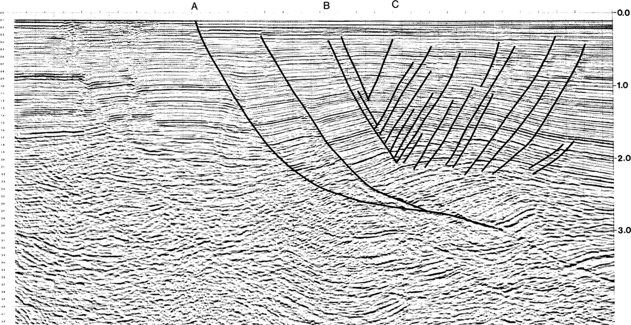
Figure 11-12 Jebco Seismic Inc. line from Brazos Ridge imaging Corsair fault (sp A), rollover structure, and downward dying antithetic and synthetic faults. Some antithetics terminate along a master synthetic fault. (Interpretation by R. Bischke. From Xiao and Suppe 1990. Published by permission of John Suppe.)
From Figures 11-4c and 11-12, and our discussion of simple rollover structures, it appears likely that the master synthetic fault is related to the active axial surface that forms at the concave downward bend in the master fault. More importantly, the master synthetic fault can be observed to offset reflectors between the 1.0-sec to 2.0-sec level, but not reflectors at 2.1 sec to 2.4 sec near sp C. Notice that the bold reflector at sp C and at 2.1 sec below sp C is coherent (i.e., not displaced). A closer inspection of the master synthetic fault shows not only that the displacements decrease downward to zero but also that the displacements die upward toward the sea floor. The fact that the displacements are negligible near the sea floor is not surprising, as little time has lapsed since the most recent sediments were deposited. Our examination of the seismic lines in this area has resulted in two seemingly confusing relationships concerning the slip along the antithetics and the master synthetic fault: (1) the slip along the antithetics generally terminates at the master synthetic fault; and (2) the slip along the master synthetic fault in Figure 11-12 at first increases from shallow depths but then dies at greater depths. Where does all this slip go, and does it really go to zero? A close examination of Figure 11-12 shows that these relationships of downward-decreasing slip continue along the deep portions of the main listric growth fault shown at sp A. However, the conservation of fault displacement and the linking of faults, discussed in Chapter 10, suggest otherwise. In Chapter 10, we make the point that slip along a thrust fault need not remain constant and that the slip could totally die in the core of a fault propagation fold. We do, however, account at all times for the changes in slip and how the slip is consumed, or dissipated. In extensional tectonic areas such as shown here, this slip, which appears to vanish so abruptly, apparently follows the bedding planes. How does this process work?
Backsliding Process
One can envision these large listric growth faults as being within a large, slowly moving landslide (Xiao and Suppe 1992). As the hanging wall fault block slips, a void opens between the hanging wall and the footwall, and the overlying material instantaneously collapses along Coulomb shear surfaces, producing the rollover (Figs. 11-2 and 11-4). We learned from Figure 11-6a and b that the greater the concave bend (ϕ) in the major normal fault, the greater the rollover angle (θ). If the dip along the major fault decreases with depth, then eventually the rollover angle may increase to an angle such that the bed dip (θ) exceeds the dip on the major fault (Fig. 11-13). Frictional failure could then occur along the bedding surfaces that form the front limb of the rollover structure, and not just along the Coulomb shear surfaces. The higher the dip of the rollover structure, the closer the sedimentary beds come into parallelism with the antithetic Coulomb failure direction. At some angle of inclination, perhaps less than the Coulomb shear angle, the bedding planes are likely to present less frictional resistance than a sequence of sedimentary layers. Thus, frictional failure along the bedding surfaces would be favored over the Coulomb shear surface (of 60 deg to 70 deg), which cuts across the layering at a high angle (Fig. 11-2b). These potential bedding plane slip surfaces are likely to occur in weak layers, such as overpressured shale zones, which would present the least possible frictional resistance.
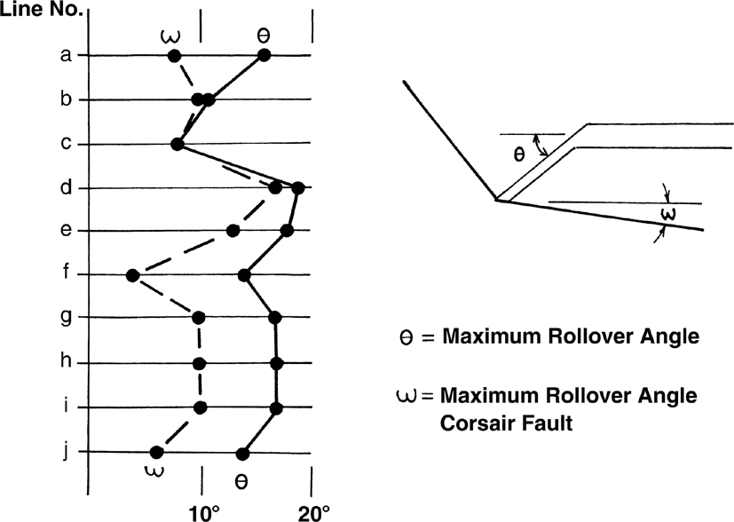
Figure 11-13 Minimum dip (ω) on Corsair fault (U.S. Gulf of Mexico) versus maximum bed dips (θ) at the front of the rollover and above its base. The frontal limb dip on the rollover structures generally exceeds the gentle dips on the Corsair fault. (Published by permission of R. Bischke.)
We therefore conclude that backsliding along bedding surfaces is a mechanism that can account for the apparent termination of the slip along the downward dying synthetic faults and antithetic faults. Using the examples of the Brazos Ridge, the backsliding appears to initiate where the rollover angle exceeds about 10 deg. The backsliding is a second-order effect relative to the total amount of slip along the major normal fault, about one part of bedding plane slip to about every seven parts of the slip along the Corsair fault. Although the bedding plane slip within the frontal limb of the rollover structure is small compared to the total slip, we shall see that it can have a marked effect on the amplitude of the rollover structure.
Backsliding Model.
Exactly how does this backsliding mechanism operate? We present two examples: the first outlines the backsliding process, and the second, a more realistic model, assumes that the backsliding consumes about 1 part in 10 of the amount of slip that occurs along the major detachment fault. Depending on geological conditions, however, backsliding may at times be the dominant process.
Figure 11-14 illustrates the backsliding mechanism. Initially, slip along the master fault must occur to an extent such that a critical rollover failure angle is exceeded (Fig. 11-14a). This critical failure angle depends on local geological conditions, such as the pore pressures, and is likely to vary from area to area. As the pore pressure is unlikely to be large in pregrowth sediments, backsliding is most likely to occur within the growth sedimentary package. At some time, a weak rock, such as an overpressured shale, moves through the concave upward bend in the normal fault surface. When this occurs, an increment of backsliding along the bedding surfaces that comprise the frontal portions of the rollover structure fills the lower part of the void created by the basinward sliding (Fig. 11-14b). Initially, the plane of detachment propagates along the bedding plane surface and, in the case of the Brazos Ridge, up to the master synthetic fault. At this location, the synthetic shear associated with the concave downward bend in the major fault turns the strata downward in the basinward direction and forms the upper portions of the rollover (Figs. 11-4c and 11-12).

Figure 11-14 Backsliding model in growth sedimentary section. (a) Uniform shear along bedding surfaces causes the hanging wall to detach from the undeformed footwall wedge. (b) The backsliding forms an antithetic fault and opens a void along the newly formed fault surface. (c) The upper void is filled by synthetic Coulomb collapse along a basinward-dipping shear band. The balanced model forms a keystone and downward dying antithetic and synthetic faults. (Published by permission of R. Bischke.)
At the position of the master synthetic fault, the shear within the weak horizon can follow one of four possible paths. First, the propagating bedding plane slip (overpressured) could also turn downward and follow the bedding surfaces across the top of the rollover structure. This possibility seems unlikely, as large amounts of energy would be required. Second, the propagating slip could cut across the more gently dipping bedding surfaces located near the top of the rollover to a pre-existing antithetic fault (plane of weakness), and then follow the older antithetic fault to the surface. This would create small, triangular-shaped structures. Third, at the position of the master synthetic, the growing bedding plane fault could follow a Coulomb failure surface up to the sea floor, creating a new antithetic fault (Fig. 11-14b). This deformation path appears to be the mechanism of least resistance and the path most favored by many compensating faults. This mechanism would also result in antithetic faults that appear to terminate along the master synthetic, which are normally observed on our Brazos Ridge seismic section example. Fourth, the hanging wall block above the bedding plane detachment and the major fault and master synthetic fault could detach and slump toward the major fault (not shown in Fig. 11-14). This mechanism would produce a surface of detachment along the master synthetic. This mechanism could be a dominant process in certain areas. We favor the third, and to a lesser extent, the second mechanism to explain the observed antithetic faulting that we have studied in examples such as the Brazos Ridge.
The third mechanism would cause another void to open along the newly formed antithetic fault (Fig. 11-14b). This hole can be filled only by collapse along the basinward-dipping Coulomb failure surfaces (Fig. 11-14c), forming a keystone structure. According to the balanced deformation model just described, another increment of backsliding will result in the formation of another antithetic, which forms above the master synthetic and the previously formed antithetic.
Another consequence of this model is that the bedding plane slip is likely to occur along shale horizons that could be related to fluctuations in sea level (Payton 1977). As a result, the intervening horizons are more likely to contain sands, or reservoir rock. Notice in Figure 11-12 that the antithetic faults die downward into a unit of semicoherent reflections between 2.1 sec and 2.4 sec. This unit is an overpressured shale, and we have observed normal faults that die into overpressured shale intervals in other structures.
Example from Corsair Trend.
A more realistic, generic example is illustrated in Figure 11-15. Here the major fault initially dips at 45 deg, decreases to 10 deg on the flat, and then steepens basinward to 20 deg. This fault configuration is similar to the shape of the Corsair fault in Figure 11-12. Also, the Coulomb failure angle is assumed to be 70 deg and the growth phase of the sedimentation to begin at Horizon 1 (Fig. 11-15a). In Chapter 13, we describe how to distinguish the growth interval from the nongrowth interval using growth plots. Since the sediments deposited beneath Horizon 1 are pregrowth sediments, and since the backsliding mechanism is likely to initiate in an overpressured horizon, the backsliding process is not likely to begin until a critical dip angle is reached within the growth sediments. At this stage, the first increment of backsliding occurs and a keystone structure forms (Fig. 11-15b) at Horizon 1. Notice in this example that the distance between the concave upward bend and the concave downward bend in the fault is greater than in the example in Figure 11-14.

Figure 11-15 (a)–(i) Generic model of the Corsair fault illustrating the progressive development of downward dying antithetic and synthetic faults through growth stages 1 to 7. (Published by permission of R. Bischke.)
Additional sliding along the major fault produces the geometry present in Figure 11-15c, and another increment of backsliding results in Figure 11-15d. The backsliding has the effect of creating keystone blocks that become younger upward as the blocks grow larger. The basinward sliding along the major fault has deactivated the antithetic fault that formed in Figure 11-15b, and this antithetic fault stopped growing after Horizon 2 was deposited (Fig. 11-15c) and was buried by the more recent growth sediments. The backsliding also has the effect of reducing the rollover amplitude. After the deposition of Horizon 4, the geometry appears as shown in Figure 11-15e. At this stage, the lower two antithetic faults, which formed during the interval of time that Horizons l to 3 were deposited, have moved through the locus of deformation (active axial surface) that is associated with the concave downward bend in the major fault. The clockwise shear associated with this deformation has the effect of slightly rotating the antithetic faults clockwise (Fig. 11-15e). During the interval of time that Horizon 5 is deposited (Fig. 11-15f), slip along the major fault has advanced to the stage that the newly forming antithetics initiate to the right of the clockwise shear-active axial surface. Thus, the antithetics that form after the deposition of Horizon 4 will not be rotated clockwise by the concave downward bend in the major fault (Fig. 11-15g). Additional increments of backsliding are shown in Figure 11-15h and i.
Figure 11-15i is a generalization of the deformation that occurred during the deposition of Horizons 1 through 7. Dashed lines are drawn at the base of the antithetic faults where the slip entered the bedding planes and at the top of the antithetic faults where they ceased to grow and became inactive (Fig. 11-15i). These lines can be considered axial surfaces that are associated with the growth phase of the antithetic crestal faulting and the formation of the keystones (Tearpock et al. 1994).
Again, notice that the more recent antithetic faulting and keystones form to the left of the older rollovers. If this model is correct, then it can be tested by data. Figures 11-16 and 11-17 are two seismic lines from the northern Gulf of Mexico and Brunei (Southeast Asia) respectively. On both of these lines, the antithetic faults have a tendency to be younger upward and to be older in the deeper sediments. The pattern of downward dying faults and keystone blocks is similar to our example in Figure 11-15.
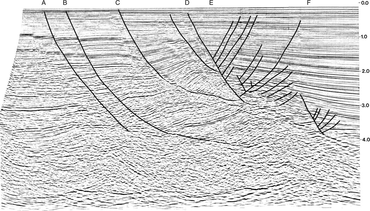
Figure 11-16 Jebco Seismic Inc. migrated line of Brazos Ridge showing antithetic faults that die with depth into the sedimentary basin. Corsair fault is imaged at sp C and two other less active faults at sp A and B. (Based on unpublished work of Xiao and Suppe. Published by permission of John Suppe.)
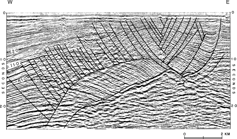
Figure 11-17 Seismic line from Brunei (Borneo) showing antithetic faults that appear to terminate along bedding surfaces. The antithetic faulting also dies with depth into the basin. (Published by permission of Muzium Brunei.)
Let us briefly review the consequences of the above-described deformation.
Growth antithetic faults form basinward and above synthetic faults located near the crests of rollovers.
The antithetics become younger upward with the older antithetics being positioned basinward and terminating at a deeper level.
Slip along the master synthetic may die with depth, and slip along the antithetic faults appears to terminate at the position of the master synthetic.
The deformation mechanism forms a keystone structure, or a graben, which with the antithetic faults has the effect of reducing the amplitude of the rollover structure.
The deformation and sedimentary mechanisms form faults that die in both the upward and downward directions.
The process may be controlled by the sedimentary cycle.
Three-Dimensional Effects and Cross Structures
Our observation of the Brazos Ridge tie lines revealed the existence of previously unreported cross structures, or transverse structures, within the rollover structure. As these cross structures determine the position of structural highs (closures), cross structures may play a fundamental role in locating closures in other rollover structures. In fact, all the Brazos Ridge closures that we studied could be located directly from strike lines (tie-lines) or from fault surface maps.
Many geoscientists, however, may mistrust 2D regional strike lines, and this is most unfortunate. They correctly reason that collecting data parallel to strike of a steeply dipping surface, such as the Corsair fault, is like collecting data from a roof. For example, seismic energy from the up-slope portion of the roof returns to the receiver, while the energy returning from directly beneath the receiver is deflected down-slope. Thus, in regions of structural dip, the energy recorded on 2D strike lines comes from out of the plane of the seismic section and is called sideswipe. Consequently, reflections on strike lines are difficult to depth-correct.
Nevertheless, our experience has led us to conclude that strike lines can be used to correctly interpret data. Strike lines may not image structures in their correct location, but we take the position that often more can be learned from strike lines than from dip lines, even though strike lines are generally more poorly imaged relative to dip lines. Indeed, strike lines look like dip lines with one additional advantage. Strike lines also image the cross structures. We make this point for the following reason. The location of all the rollover closures along a 25-mi section of the Brazos Ridge that we studied, and this includes five rollover structures and four major gas fields, can be predicted from a single strike line. In frontier areas subject to extension, the use of regional strike lines can rapidly locate structural highs within a large rollover structure and save the expense of acquiring numerous unnecessary dip lines.
The Brazos Ridge strike lines clearly image the Corsair fault and a number of other faults on a deeper structural level. In Figure 11-18, the Corsair fault is imaged as a distinct boomer (strong reflection) between the 2.3-sec to 2.7-sec level to the right of sp C. The fault surface is not planar. The Corsair is level between sp C and sp D, but then it deepens to 2.7 sec at sp E. The Corsair fault is seen to surface in Figure 11-18 at about sp A (0.2 sec). You can follow this fault downward to about the sp B area, where another deeper fault is observed to deform, or roll over, the Corsair fault, analogous to the geometry in a compressional duplex (Chapter 10). This deeper fault continues beneath the Corsair to perhaps the 3.55-sec level, where it levels off (at sp D). On the dip lines, this and other deeper faults can be observed to surface to the north or landward of the Corsair fault, to dip beneath the Corsair fault, and to be presently active, although at much lower slip rates (Fig. 11-16, sp A and B). In Figure 11-16, the Corsair fault is seen to surface at sp C. On the strike lines, these deeper faults can be observed to intersect the Corsair fault (Fig. 11-18, sp B), to offset the fault, or to form cross structures.
Figure 11-18 Jebco Seismic Inc. strike line along Corsair fault. Deeper faults have deformed the Corsair into a series of highs and lows that create cross structures on the fault surface map (Fig. 11-19). The low on the Corsair fault at sp B creates Chute 1 on Figure 11-20. (Published by permission of Jebco Seismic Inc., Houston, Texas, USA.)
These cross structures trend subperpendicular to the Corsair fault and deform and partition the footwall into a series of high-gradient and low-gradient areas (Fig. 11-19). On a regional scale, the series of highs and lows on the Corsair fault, which are caused by the major subfault deformation, are bounded by the cross structures (Fig. 11-20). The low-gradient, shelf-like, or “flat” areas on the Corsair fault produce what we term bows on the fault surface. Bows are known in the U.S. Gulf of Mexico to be a key indicator of a petroleum trap. We propose the term chute for the higher gradient regions of indentation into the fault surface. The strike line (Fig. 11-18) images chute 1 (Fig. 11-20) at sp B.
Figure 11-19 Fault surface map of a portion of the Brazos Ridge. The structural contours deepen toward the lower portion of the diagram. The cross structures segment the fault surface map into a series of low-gradient areas (bows) and high-gradient areas (chutes). (Prepared by W. L. Keyser. Published by permission of Texaco USA, Eastern E & P Region.)
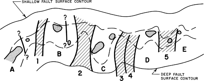
Figure 11-20 Location of chutes and bows. The chutes exist as intrusions into, and the bows exist as protrusions upon, the fault surface map (Fig. 11-19). Five bows and chutes exist along trend, with chutes 3 and 4 being a double chute. (Published by permission of Texaco USA, Eastern E & P Region.)
Finally, we demonstrate that the general position of the rollover structures can be predicted from the fault surface map of the Corsair fault (Fig. 11-19), with the bows (lowest gradient areas) on the fault surface corresponding to the position of the structural highs within the rollover structure and the chutes (higher gradient areas) corresponding to the position of the saddles between the structural highs. These relationships are shown in Figure 11-21, which is a restored time map of a horizon within the rollover structure. The map was restored to a common level by simply closing the faults. A comparison of Figure 11-21 to Figures 11-19 and 11-20 demonstrates that the bows correlate to the position of the structural highs, whereas the chutes correlate to the saddles. Thus, rollover closures can be located from fault surface maps, which further demonstrates the value of constructing these maps (Chapter 7).

Figure 11-21 Partially restored horizon time map. The structural highs correspond to the position of bows, whereas the saddles correlate to the chutes. (Published by permission of Texaco USA, Eastern E & P Region.)
What does the saddle geometry look like in 3D? Figure 11-22 is a 3D perspective view of the flanks of two structures within a large rollover structure, based on a study of axial surface deformation in the Central Sumatra Basin, Indonesia (Shaw et al. 1997). The fault surface contains a central low, or chute, and the chute is bordered on its flanks by two fault surface highs. As the hanging wall block moves down the fault surface, the displaced horizons conform to the shape of the 3D low in the fault surface, forming a saddle and the flanks of the adjoining structures, as depicted in the inset in Figure 11-22. The geometry resembles that observed on the strike line (Fig. 11-18) between sp D and sp E, where the flank of a closure in the hanging wall block is imaged. The structures flanking the low dip toward the chute in the fault surface (Fig. 11-22).
Figure 11-22 Perspective view of a 3D structural saddle based on a fault surface map from Central Sumatra Basin, Indonesia. The low area on the fault surface generates a structural low. (Modified after Shaw et al. 1997; AAPG©1997, reprinted by permission of the APPG whose permission is required for further use.)
Strike-Ramp Pitfall
We discuss the necessity of constructing accurate maps throughout this book, and we emphasize that here by presenting examples of the pitfall in interpreting strike-ramps between en echelon normal faults, which are common in extensional terranes (Tearpock et al. 1994). We demonstrate how to recognize, locate, and avoid this costly pitfall. We have observed this problem and its resultant dry wells on a number of 2D and 3D data sets. The examples illustrate the necessity of constructing accurate maps of subsurface faults.
Strike-ramps form along arrays of normal faults that contain en echelon offsets, or stepovers (Morley et al. 1990; Peacock and Sanderson 1991). Strike-ramps are commonly ubiquitous features on extensional data sets. Examine the air photograph shown in Figure 11-23, taken from the Yucca Mountains, Nevada (Ferrill et al. 1999). Notice how the Boomerang fault almost connects to the uppermost extension of the Fatigue Wash fault, but no connecting fault links the two fault systems to form a two-way fault closure. On 3D data sets, the seismic data may become semicoherent, or deteriorate, where two faults overlap, perhaps due to the fault shadow effect. If this occurs, then structural horizon mapping may result in the mapping of two fault surfaces as a single fault surface. In addition, on 2D and 3D seismic data sets, structural aliasing can result in mapping the two overlapping faults as one fault (Fig. 11-24a and b). Furthermore, this overlap has a limited lateral zone. Even if the data are good, en echelon faults may be overlooked if the interpretation is based on insufficiently close seismic lines.

Figure 11-23 En echelon normal fault surfaces from Yucca Mountains, Nevada, USA, showing faults and fault offsets in bold lines. An unfailed block, or strike-ramp, separates the Boomerang fault from the Fatigue Wash fault. Failure of the block between the Fatigue Wash and Northern Windy Wash faults creates the West Ridge cross fault. In the subsurface, a structural geometry identical to the Yucca Mountains normal fault system would trap hydrocarbons in the block downthrown to the West Ridge connecting fault system, but not in the block between the Boomerang and the Fatigue Wash Faults. (From Ferrill et al. 1999 Published by permission of Elsevier Science, Journal of Structural Geology.)
Figure 11-24 (a) Two en echelon faults die out in opposite directions, creating a strike-ramp. The unfaulted ramp is incapable of trapping hydrocarbons. An improperly spaced 2D data set, structural aliasing, or poor 3D seismic data in the area of fault overlap could result in the prospect shown in (b). (b) If fault surface maps are not constructed, then a combination of incomplete seismic control, structural aliasing, or poor 3D seismic data can create a nonexistent prospect. (Published by permission of R. Bischke.)
Notice on Figure 11-24a that the strata downthrown to the overlapping faults form a structural low relative to the upthrown strata. Where Fault 1 dies out, or loses displacement to the east, Fault 2 increases in displacement to the east. This reversal of displacements between the offsetting fault surfaces causes the strata within the overlap area to dip to the west, forming a strike-ramp. The pitfall is that this ramp may or may not contain a fault that would form a three-way fault closure (Brenneke 1995).
Let us assume that the strike-ramp shown on Figure 11-24a is within a 3D survey area, that a fault shadow effect causes the data to deteriorate between the offset fault surfaces, and that the data were interpreted along equally spaced lines. If on the 3D data set the horizontal distance between the two overlapping fault surfaces is large, then seismic horizon mapping should detect the strike-ramp. On narrower strike-ramps, however, structural horizon mapping of the offset fault surfaces is subject to possible fault miscorrelation problems. Geoscientists may assume that the fault surfaces are throughgoing and, in this case, the deterioration of the seismic data set may not resolve that two faults are present. If the geoscientist connects Fault 1 to Fault 2, then the result is a nonexistent prospect based on a three-way closure (Fig. 11-24b). In practice, the data are commonly incoherent between the offset fault surfaces, so in such a case, interpreting every line on a 3D data set may not even resolve this problem.
How does one locate, recognize, and resolve fault correlation problems? Figure 11-25 shows a fault surface map that contains two en echelon faults, which are incorrectly mapped as a single fault. Can you detect the strike-ramp between the two faults? The strike-ramp exists as a minor bend or curve on the fault surface map (Brenneke 1995).
Figure 11-25 Fault surface map of two en echelon fault surfaces mapped as a single fault surface. Bend in fault surface map suggests the possible presence of two faults that do not intersect rather than one fault. Map is in two-way time (msec). It was generated using a triangulation algorithm that does not smooth through bends in fault surfaces. Compare to the coherency cube display in Figure 11-26 that clearly shows the presence of two separated faults. (Published by permission of R. Bischke.)
We are aware of two methods to prevent this costly pitfall, both of which involve fault surface mapping. Geoscientists can analyze 3D coherency data over many time slices (Fig. 11-26). Coherency data commonly image the en echelon offsets associated with strike-ramps, particularly on the shallow structural levels. When interpreting seismic data, assign a fault segment to every fault that exists on the multilevel time slices. These interpreted fault segments on the time slices represent strike (trace) segments relative to the dip profiles. Thus, faults observed on time slices easily tie to faults observed on dip profiles.

Figure 11-26 Strike-ramp on coherency cube data taken from St. Charles Ranch, Texas. Just above the dashed line, the en echelon pattern of the faults is evident. The dashed line represents a fault surface contour on Figure 11-25, where the curvature of the contours is a clue to possible en echelon faults. (Published by permission of R. Bischke.)
Lacking coherency data on 3D data sets, or when using 2D data, you can locate en echelon offsets by constructing fault surface maps, as described in Chapter 9. If the fault surface map contains a kink or a bend, as in Figure 11-25, then en echelon faults may be present. Two overlapping fault surfaces, separated by a significant horizontal distance, will contain a contouring bend if mapped as a single fault surface. However, two closely spaced faults may exhibit only a subtle kink or bend in the fault surface. When using 3D data, we can readily solve the problem of distinguishing between a gentle bend in a single fault from an en echelon offset of two fault surfaces. Construct several arbitrary lines across the kink or the bend in the fault surface, at oblique angles to the kink. Where strike-ramps are present, these arbitrary lines will commonly encounter regions of coherent data in the areas where the two fault surfaces do not overlap. Accordingly, two faults, and not one fault, will image on the arbitrary lines.
In order to solve the strike-ramp problem on 2D data sets, properly oriented oblique or dip profiles must exist that cross both faults. These lines may not exist. Thus, be suspicious of any bend, kink, or curve in a normal fault surface that acts as a potential trapping fault for a prospect. Risk this bend in the fault accordingly. An additional line or two may need to be acquired to resolve the problem.
Alternatively, additional motions along the strike-ramp may generate faults that link two originally separate faults, creating a fault trap (Tearpock et al. 1994). The probability of an accumulation in this type of trap depends on the timing of these younger faults. Chapter 13 in this book and Tearpock et al. (1994) present methods for studying fault timing.
Geoscientists should exercise care when interpreting faults and constructing fault surface maps. Geoscientists loop-tie fault surfaces maps for the same reason that they loop-tie horizon surfaces: to make sure they remain on the same fault. Also, consider that on 3D data sets, randomly placed arbitrary lines may or may not locate the strike-ramps. Strike-ramps that exist along faults that constitute the same fault system are often subtle features on 3D data sets. Geoscientists must know where to place the arbitrary lines in order to demonstrate that a trapping fault exists. Correctly interpreted and loop-tied fault surface maps show geoscientists where to place the arbitrary lines. Fault surface mapping also reduces the horizon mis-tie problem, often saving time. The final product is a higher quality interpretation and prospects.
Compaction Effects Along Growth Normal Faults
We present a theory developed by Xiao and Suppe (1989), which explains why some growth normal faults are listric (concave upward) or antilistric (concave downward). When using depth-corrected seismic data, it is apparent that faults are commonly listric in shape through predominately shale sections and turn antilistric into thick sand packages. Generally, about 20% to 30% of the faults in an area like the northern Gulf of Mexico coastal region are mapped as antilistric, whereas in specific areas like Brazos Ridge, the majority of the antithetic faults are antilistric. We stress that the following techniques for projecting faults into poor data areas apply only to growth faults, which were active when the sediments were being deposited, but not to the sections of those faults within pregrowth sediments deposited prior to the normal faulting. In other words, these techniques apply only to those portions of a fault that were active during deposition.
Furthermore, this method uses the true dip of a fault, so any seismic profile used for data must be dip-oriented (perpendicular to the strike of the fault), depth-corrected, and as close as possible to true scale. Similarly, cross-sections must be dip-oriented and at true scale.
An understanding of the change in fault shape with depth is critical in applying the fault projection technique. Consider two small columns of material, column A located at the sea floor and column B located at depth, as illustrated in Figure 11-27. Column A is just recently deposited and not subject to significant compaction, whereas column B is buried and is compacted. Initially, column A has width ΔX and an initial porosity of ϕ0 If we define the height of column A as ΔY, then the initial dip of the growth normal fault relative to the footwall is defined by

Figure 11-27 Compaction and burial along a growth normal fault. Element A at the sea floor compacts to the geometry present at B. These relationships are taken relative to the compacted footwall. (From Xiao and Suppe 1989. AAPG©1989, reprinted by permission of the AAPG whose permission is required for further use.)

After burial, column A will dewater and compact and take on the shape of column B (Fig. 11-27).
Column B has a buried width, height, fault dip, and porosity of ΔX′, ΔY′, θ, and ϕ respectively. Therefore, the fault dip at B is defined as
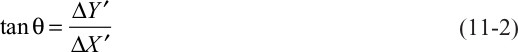
However, the compaction primarily affects the height and not the width; therefore,
and thus, using Eqs. (11-1) and (11-2),
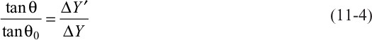
where θ = bed dip
As porosity controls the extent of compaction (Baldwin and Butler 1985), this mass conservation formula written in terms of solid volume is
and from Eqs. (11-4) and (11-5), we derive
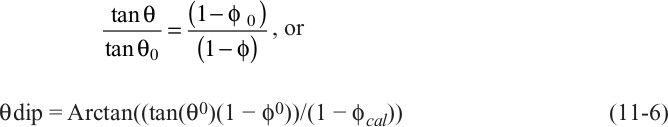
where
Therefore, if we are able to predict the initial fault dip (θ0) and initial porosity (ϕ0) along with the porosity (ϕ) of the rock at any given depth level, we can determine the approximate fault dip (θ) at any level of interest (Xiao and Suppe 1989) (Fig. 11-27).
The process of dewatering and compaction is rapid, occurring within about the upper 700 ft (Baldwin and Butler 1985), so any compaction equation is controlled primarily by the porosity, which is in turn related to the sandstone/shale ratio. Thus, if the depths of a normal fault are known in each of several neighboring wells, and if the sandstone/shale ratios are known from local or adjoining footwall well logs, then the fault shape and its location can be extrapolated between the adjoining wells using Eq. (11-6). Case histories of the process are presented later in this section.
Before applying Eq. (11-6) to an area, we must be able to calculate the amount of porosity to be expected in sandstone and shale horizons at any given depth. Porosity/depth equations are dependent on the region being studied (Baldwin and Butler 1985). These equations represent the average porosity of sandstone or shale at any given depth, so determine these relationships by using local data. The porosity/depth equations represent averages, so results will also represent averages.
For the U.S. Gulf Coast, the following empirically derived sandstone and shale porosity/depth equations can be applied (Xiao and Suppe 1989). For shale,
where

For sandstone, Eqs. (11-8) through (11-10) apply:
and
Alternatively, you may use the following equation (Atwater and Miller 1965).
where

From Eq. (11-9) we can determine that the initial sandstone porosity is about 39% by setting the depth to zero. Porosity/depth equations for areas other than the Gulf of Mexico are presented by Baldwin and Butler (1985) and Sclater and Christie (1980).
The technique can now be applied. First, the sandstone portions of a well are determined by locating the sandstone and the shale base lines from spontaneous potential (SP) logs. Common industry practice suggests that sandstones exist wherever the SP log exceeds 25% of the distance between the sandstone and shale baselines (Fig. 11-28). Values of less than 25% on the divided SP log are taken to be shale (Schlumberger 1987). Second, a “splicing method” is employed, using Figure 11-29. In those depth intervals that have been determined from the SP log to be sandstone, use Eq. (11-8), (11-9), or (11-10), and use Eq. (11-7) in those depth intervals that represent shale.
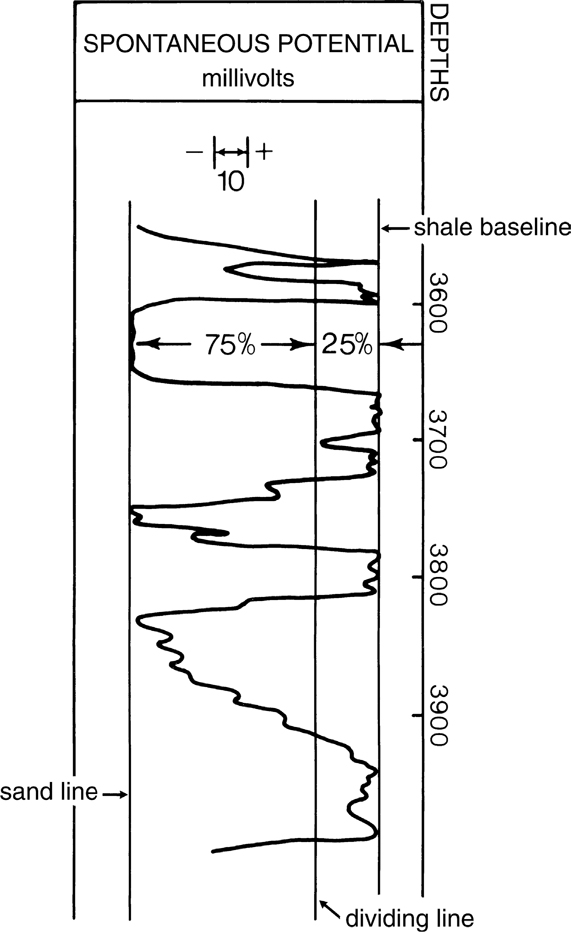
Figure 11-28 Relationships utilized to determine sand/shale ratios. Sand is present wherever the SP log deviates more than 25% off the shale base line. (From Xiao and Suppe 1989. AAPG©1989, reprinted by permission of the AAPG whose permission is required for further use.)

Figure 11-29 The splicing method for estimating fault dips from sand/shale horizons determined from SP logs. (From Xiao and Suppe 1989. AAPG©1989, reprinted by permission of the AAPG whose permission is required for further use.)
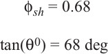
Equation (11-6) is also dependent on the initial fault dip and initial porosities. As an example, for the northern Gulf of Mexico these values have been empirically determined to be 67.5 deg for initial fault dip, and 39% and 68% porosity for sandstone and shale, respectively (Xiao and Suppe 1989). You may wish to confirm these initial values from local data prior to applying Eq. (11-6) to your area of interest. We have now determined the sandstone and the shale portions of the sedimentary section from the SP logs and can calculate their average porosity at any given depth from Eqs. (11-7) to (11-10). Therefore, we can now calculate the average fault dip (θ) at any depth from Eq. (11-6) and the splicing method. These formulae were tested with good results in a number of examples in the Gulf of Mexico, such as the one shown in Figure 11-30.
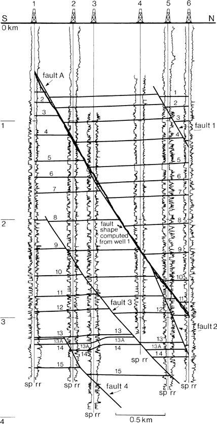
Figure 11-30 Test example for projecting fault dips between wells. The SP log from Well No. 1, the fault dip (Fig. 11-27), and the porosity/depth equations are utilized to predict the shape and position of Fault A with depth. (From Xiao and Suppe 1989. AAPG©1989, reprinted by permission of the AAPG whose permission is required for further use.)
In areas of poor seismic data, or in areas with well log data and limited seismic data, the technique can be used to help interpret the shape of important growth faults. The shape of a fault with depth may be important in generating a prospect, designing a prospective well location, or the determination of reserves based on the areal extent of a reservoir.
Perhaps a prospect is under evaluation and the location of the trapping fault is of critical importance. The method can be used as a “quick-look” technique (Tearpock et al. 1994) to evaluate the presented interpretation and, in particular, the shape and location of the trapping fault.
Prospect Example
A good application of this method arises when analyzing a prospect. Examine Figure 11-31, showing Well No. 1, which penetrates a large growth fault, and Well No. 2, which has a discovery at the D Sand level on a rollover structure. Seismic data from this area are not of the best quality, but they image gentle south dips. The proposed well, to be drilled up-dip of the discovery well, looks like a lead-pipe cinch! Would you participate in the proposed well? If not, why not?
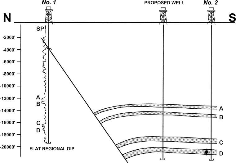
Figure 11-31 Proposed well position located up-dip of the producing Well No. 2, and downthrown to a planar fault surface that intersects Well No. 1 at −4000 ft. Quick-look techniques can determine structural viability of the proposed production well. (Published by permission of R. Bischke.)
Let’s do a quick examination of the cross section in Figure 11-31. We first observe that the normal fault is planar in shape, dipping at an angle of about 55 deg. The discovery and proposed wells appear to be in the hanging wall rollover anticline formed by the fault, which is penetrated by Well No. 1.
Several questions come to mind. Why is the fault in Figure 11-31 not listric? Why do the beds dip or roll toward a fault surface that is a planar surface? Geoscientists know that rollover structures are associated with listric fault surfaces; that is, rollover structures form above fault surfaces that are not planar. In the section on the origin of rollover in this chapter, we demonstrate that only above listric fault surfaces do hanging wall strata form a rollover anticline.
Let’s take a look at the fault surface shown in Figure 11-31 and refer back to Figure 11-29. Figure 11-29 allows us to estimate fault dips from lithology. The lithology in the footwall of the fault in Well No. 1 allows us to predict the dip and shape of the fault. Well No. 1, which penetrates the fault near −4000 ft, contains about 50% sand in the footwall block between the −4000-ft and −8000-ft levels (−1200 m to −2400 m). The average depth of the sandy section is −6000 ft (−1800 m). On Figure 11-29, a fault at a depth of −6000 ft (−1800 m) in a 50% sand section will dip at an angle that lies halfway between the fault shape in pure sandstone and the fault shape in pure shale. We can fit a protractor to this figure to obtain a fault dip of about 55 deg. The fault shown on Figure 11-31 dips about 55 deg between −4000 ft and −8000 ft, exhibiting good agreement between observation and theory.
Notice that Well No. 1 penetrates a predominantly shale section below −8000 ft (−2400 m). Thus, the footwall section below −8000 ft should be subject to significant compaction. Faults in compacting shales will dip at gentler angles than faults traversing sand-rich sections. Let’s take another look at Figure 11-29, but this time we assume a pure shale section between −8000 ft and −20,000 ft (−2400 m to −6100 m). The average depth of this pure shale section is about −14,000 ft (−4250 m). Fit a protractor to the fault shape on the pure shale curve (Fig. 11-29) at an average depth of −14,000 ft. Figure 11-29 predicts that the fault will dip at an average of 40 deg below −8000 ft. If the fault dips at an average of 40 deg below −8000 ft, then the fault should follow the path shown in Figure 11-32. The listric bend in the fault causes the strata to roll toward the fault and to form a rollover anticline in the hanging wall block (see section on origin of rollover). Furthermore, the listric shape of the fault causes the strata to dip at a higher angle than those shown in Figure 11-31 and causes the fault to be farther to the south than previously interpreted. The result of our quick analysis is to predict the possibility that the productive D Sand will be faulted out in the proposed well (Fig. 11-32). What appeared at first to be a sure thing may not be. An alternative to the quick-look method is to use a spreadsheet and the procedures outlined in this section to write a program using Eqs. (11-6), (11-7), (11-8), (11-9), and (11-10). The program can be used to predict the fault dip through a varying sandstone/shale section.
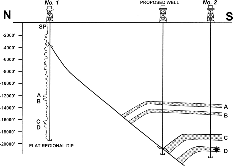
Figure 11-32 The SP log in Well No. 1 and the compaction formula result in a listric fault surface that dips at a lower angle below −8,000 ft, causing the interpreted fault to displace to the south. Listric shape of the fault surface causes the beds to roll toward the fault surface. Given this structure and the relocated fault, a good probability exists for the reservoir being faulted out in the proposed well. (Published by permission of R. Bischke.)
The importance of this example is to stress that there is often a geometric relationship of fault shape to fold shape, and it can be used when generating geologic interpretations. The cross section shown in Figure 11-31 does not conform to certain basic geologic principles. Therefore, a good possibility exists that the interpretation is in error. The error may be small or large. The quick-look technique indicates that the error, in this case, may be large enough to result in a dry hole. This quick analysis should direct the prospect generator to additional work to either substantiate the interpretation, as shown in Figure 11-32, or modify the interpretation based on the principles shown in this section on the effects of compaction on the shape of growth normal faults.
The compaction work presented by Xiao and Suppe (1989) can result in accurate predictions of fault shape where compaction is the predominant process. The method is stable and tends to average the well log data. As the method predicts the average fault dip based on the average lithology over an interval, the method averages through intervals that do not obey the idealized compaction formulae. Thus, the method tends to average out local and aberrant secondary cementation intervals that may affect the compaction curves. Deformation of the fault surface, either by salt or by another fault, may affect the results of the method.
Inverting Fault Dips to Determine Sand/Shale Ratios or Percent Sand
Inverting fault dips is a technique used to estimate the percent sand in a prospective interval, which is valuable information for a prospect. When well log data are not available on the level of interest, and provided that a normal fault is present, it may be possible to estimate the amount of sand off of a seismic line. The seismic line must be depth-corrected. With an estimate of the percent sand over the prospect area, a certain amount of risk can be mitigated, better volumetrics can be estimated, and overall economic evaluation can be improved.
Normal faults can be listric in shape and dip at lower angles with increasing depth, or the faults can be antilistric and dip at higher angles with increasing depth (Fig. 11-29). Observation by industry indicated that growth normal faults commonly dip at shallower angles in shale sections and at higher angles in sand sections (Gow 1962; Roux 1978). Industry uses this relationship between fault shape and lithology (Roux 1978) to predict sand intervals from depth-corrected seismic profiles. If on a depth-corrected, dip-oriented seismic section a growth fault steepens at depth, then the fault may be entering a sand-rich interval (Bischke and Tearpock 1993). In this section, we develop a technique based on the Xiao-Suppe equation [Eq. (11-6)] to estimate percent sand from the shape of faults on depth-corrected seismic sections.
In the Brazos Ridge area in the northern Gulf of Mexico, many of the growth normal faults at shallow depths, and within the crests of rollover structures, dip at angles of 40 deg to 45 deg, and with greater depths dip at higher angles (50 deg to 60 deg). These antilistric normal faults steepen into a known section of higher sandstone/shale ratios (approximately 1.0 to 1.5). These normal faults are the basis for a method of using fault dips to estimate sandstone/shale ratios (Bischke and Suppe l990a). The basic concept for accomplishing this task has been presented in the previous section and is implicit in Eq. (11-6).
For example, if the initial fault dip (θ0) and porosities (ϕ0) are known and if the average porosities (ϕ) are calculated at all depth levels using Eqs. (11-7) to (11-10), then the fault dip (θ) at the level of interest can be calculated from Eq. (11-6). This is the forward modeling procedure described previously. Forward modeling is more accurate than inverse modeling, and ratios such as sand/shale ratio are sensitive.
If, however, the fault dip (θ) is constrained by good depth-corrected seismic sections, then the average porosities (ϕ) for sand and for shale can be calculated from Eqs. (11-7 to 11-9) at any depth level. This is called inverse modeling, which is sensitive to measurement errors. As porosities are dependent on lithology [see Eqs. (11-7) to (11-10)], we can estimate the (sand or shale/depth curve in any area, provided that we have information on local porosity depth curves. This information can be derived from the nearest wells, which in frontier areas could be many miles from the area of interest.
First, we must initiate a sandstone/shale ratio formula. This can be accomplished using Figure 11-33. In practice, the observed height of the figure is the top and the bottom of a portion of an interpreted growth normal fault on a depth-corrected seismic section. This distance represents a column of interbedded sandstone and shale. Using a deck-of-cards analogy, the sandstone layers are removed from the deck and placed at its bottom.

Figure 11-33 An alternating sequence of sand and shale beds can be generalized into a shale interval of thickness hsh and a sandstone layer of thickness hss. As shales have a higher initial porosity than sandstones, shales compact more than sandstones. (Published by permission of R. Bischke.)
We now calculate from Figure 11-33:
where
Using the law of sines,
and substituting and rearranging yields
or
where
Sandstone/shale ratios can be converted to percent sand by the following equation:
As θsh and θss can be obtained from Eq. (11-6) and the porosity from Eqs. (11-7) to (11-10), we can calculate the average porosity, or sand/shale, curve with increasing depth.
Before proceeding to a test case, we outline a number of factors that affect the accuracy of our methods.
Inversion methods are sensitive, and errors occur when measurements are not accurate. The method is most accurate when penetrating thick sand sections interbedded with thick shale formations, such as exist in the Brazos Ridge and Segno Field examples presented in the next section (Figs. 11-34, 11-36, and 11-37).
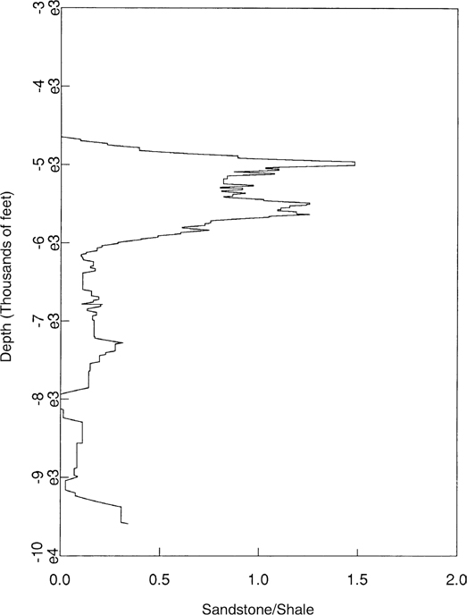
Figure 11-34 Processed sandstone/shale depth curve obtained by averaging sand/shale horizons taken from an SP log from Well No. 9 (Bischke and Suppe 1990a). The data are plotted at a frequency of two seismic wavelengths and range in depth from −3000 ft to −10,000 ft. (Published by permission of R. Bischke.)
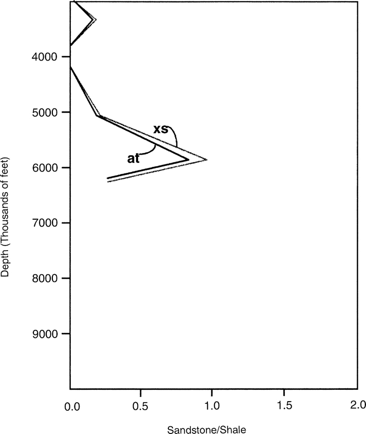
Figure 11-35 Plot showing predicted sandstone/shale depth curve derived from fault dips interpreted on seismic profile. The fault is adjacent to the well data shown in Figure 11-9 in Bischke and Suppe (1990a). The xs curve uses the Xiao-Suppe compaction equation, whereas the at curve denotes the Atwater equation. (Published by permission of R. Bischke.)
Figure 11-36 (a) Map of Segno Field, Texas, USA, with location of Cross Section A-Aʹ. (b) Section A-Aʹ shows growth fault steepening in sand intervals. As Gow (1962) noted on the section, “Note that fault plane steepens in sand formations.” (From Bischke and Tearpock 1993. Redrawn from Gow 1962. Published by permission of the Houston Geological Society.)
Figure 11-37 Percent sand plot for Segno Field growth fault, based on changes in dip of fault. Fault steepens through Yegua and Wilcox sand sections, generating a high sand percentage response from about −5000 ft to −7000 ft and below about −9000 ft. Compare calculated sand percentages to sand percentages based on log of footwall Well No. 8 (closed box bar on graph). (From Bischke and Tearpock 1993. Published by permission of the Houston Geological Society.)
Accordingly, accurate measurements are necessary.
The method applies only to growth normal faults and thus to areas that are experiencing both active sedimentation and extension.
Although the method can be applied wherever velocity information is available, the velocity function is critical to obtaining reliable results because it is used to determine depth of the fault. Velocity determinations are discussed in Chapter 5.
The method in its present stage of development involves only compaction, and thus deformation of normal faults by other processes, such as salt flow, may invalidate the method.
The method is restricted to the depth to which the seismic reflections can be resolved.
The method applies only to sandstone/shale lithologies, and not to carbonates. However, faults also steepen into carbonate reservoirs.
Example from Corsair Fault Offshore Texas
In the following test of the method from data located on the Corsair fault, Texas, we compare a depth-corrected growth normal faults to well log data (Bischke and Suppe 1900a). In order to compare observed well log results, which resolves horizons to within feet to seismic data, in which the resolution is a function of depth, the well log data must be converted to longer wavelengths. This is accomplished by first determining the sand and shale horizons from SP logs, as discussed earlier (Fig. 11-28), and then measuring the wavelength of coherent reflectors from the seismic section. The frequency content of the seismic section is thus determined. As the frequency content decreases with depth, the wavelength of the reflections increases with depth. This wavelength is then depth-corrected and passed over the SP data as a moving average, with the length of the operator increasing with depth. The result of this averaging process from an example well is the sandstone/shale depth curve shown in Figure 11-34. The processed data are near several antilithic faults located on a rollover above the Corsair fault, Texas (Bischke and Suppe 1990a, their Figs. 8 and 9). The data are plotted at a frequency of two seismic wavelengths. This long-wavelength well log data can be directly compared to normal fault calculations based on seismic data.
Typical results, calculated using Eq. (11-13) and based on a growth fault located near Well No. 9, are shown in Figure 9 of Bischke and Suppe (1990a). This fault is the closest fault to Well No. 9. The results approximate the well log data. The seismic data was processed utilizing stacking velocities. The normal fault, which terminates at a depth of −7000 ft, has been used to predict the higher sandstone/shale ratios present in the −4800-ft to −6300-ft level. Other examples, located closer to the main fault, encounter a sedimentary dumb or more precisely a prograding wedge, which has higher sandstone/shale ratios ranging from 2 to 4. The prograding wedge thins and dies out near the crest of structure. A typical calculated example is shown in Fig. 11-35, in which high sandstone/shale ratios occur near 1 between a depth of 5500 ft to 6000 ft.
Elements of the sandstone-shale theory were known to industry for many years and were applied worldwide. As a final example, we examine a field in Texas where an early form of the method was applied in the 1960s.
Example from Segno Field, Polk County, Texas.
The Segno Field rollover structure formed downthrown to an east-west trending normal fault (Fig. 11-36a). Examine the footwall portion of cross section A-A′ constructed from dense well control on the eastern flank of the field (Fig. 11-36b). This section from Gow (1962) through the Tertiary Jackson, Cook Mountain, Sparta, and Weches shale sections shows that the normal fault dips at angles of 30 deg to 40 deg. Gow wrote on the profile, “Note that fault plane dip steepens in sand formations” (Gow 1962). In the Yegua and Wilcox sand sections the fault surface steepens to about 50 deg to 55 deg (Fig. 11-36b).
A change in fault dip angle from 30–40 deg to 50–55 deg is typically apparent on depth-corrected seismic profiles. Indeed, Roux (1978) presents an example of a fault that changes dip through a thick sand and shale section on a vintage seismic time profile. This profile is in Lowell’s book on structural styles (Lowell 1985). Industry recognized, and at times used, this “change in fault dip technique” to locate sand sections during the 1960s and 1970s. Subsequent bright spot analysis apparently replaced the technique, but geoscientists are again using the technique where direct hydrocarbon indicators are not applicable or not in support of amplitude versus offset (AVO) analysis.
We obtained a seismic line that crosses the crest of the structure. The line was digitized and depth-corrected using interval velocities. Interval velocities approximate true velocities and are always available to the geoscientist. On the profile (Fig. 11-36b), the fault dips at high angles through the Yegua and Wilcox sands and at less steep angles through the Jackson, Cook Mountain, and Sparta shale sections (Bischke and Tearpock 1993). After picking the fault on the vintage seismic line, the inflection points on the fault surface were depth-corrected for input into a sand percentage prediction program. This program uses formulas presented in the previous section. Program results shown in Figure 11-37 are comparable to Well No. 8 in the footwall block (Fig. 11-36a), located adjacent to the seismic line (Bischke and Tearpock 1993). In Figure 11-37, the diamond-shaped bar on the left shows the resulting computations from the Atwater-Miller sand compaction formula [Eq. (11-10)], whereas the open box bar on the right defines the Xiao-Suppe compaction curve results [Eqs. (11-8) and (11-9)]. The Atwater-Miller sand compaction formula is more conservative than the Xiao-Suppe formula. The closed box bar (middle) is the percent sand based on the Well No. 8 log.
When subject to computation, the interpreted fault trace predicts a sand response on the level of the Yegua sand between the depths of about −5000 ft and −7000 ft. The Atwater-Miller and Xiao-Suppe bars bracket the sand percentage in Well No. 8 and predict a sand percentage of about 60% (Fig. 11-37). Between the −5000-ft and −6700-ft depths in Well No. 8, the sand percentage is about 60% (Bischke and Tearpock 1993). An examination of Figure 11-37 indicates that a shale section should exist at about the −7000-ft to −8800-ft level and that sand should exist below −8800 ft. Well No. 8 contains shale between −6700 ft and −8200 ft before encountering the Wilcox sand (Fig. 11-36b). These estimates, which are a good match to the well data, are based on imprecise interval velocities, and better velocity estimates and seismic data should improve the depth percent sand and sandstone/shale predictions.
The method works best on seismic sections where you can pick the fault trace accurately and where thick sand and shale sections are present. Fault surfaces also respond to interbedded sand/shale sections, and the section need not be predominantly sand (Bischke and Tearpock 1993; Tearpock and Bischke 1991). Why drill a well to a depth of 20,000 ft if there is no direct evidence for sand at that level, without first using fault dip analysis to help reduce your sand risk?
This method has application to petroleum exploration, as was recognized by industry years ago (Gow 1962; Roux 1978). Normally, when a well is drilled, one of the least known parameters is the sand/shale ratio of the reservoir. As the section in the Segno Field example contains shale from −7000 ft to −8800 ft (Fig. 11-37), the method also produces estimates for seal thicknesses. Such information can be used by a geoscientist or engineer to better determine the target depths for wells and to improve the estimates of potential reserves prior to drilling. The method can be applied to the third dimension, so 3D percent sand maps can be constructed to better select well locations.
We have seen examples of exploration well locations being moved by as much as 1000 ft on the basis of this analysis. If a prospect has good structural closure over a large lateral area, the specific choice of the actual well location may be based on where the prospective intervals have the highest percent sand. This technique can be used, under the circumstances discussed, to make such determinations. All that is required to apply the method is an array of small antilistric, growth normal faults. The usefulness of the method increases as well control becomes limited and the distance between wells increases.
Using Structural Relief and Throw to Predict the Downthrown Stratigraphic Section
This section discusses several methods that may be used in some cases to predict the downthrown stratigraphic section on deep rollover structures. The requirements are a depth-corrected seismic section that images the master (major) fault surface, the general geometry of the structural relief of the hanging wall rolled over, anticlinal beds, and the stratigraphy of the upthrown beds. These beds are typically at the depths to known sand intervals, or sandy shale horizons that contain a high percentage of total organic carbon content (%TOC). These intervals need not be drilled downthrown to the fault. One method shows how the expanded downthrown stratigraphic section may be predicted at greater depths by measuring the R/T ratio, which is the downthrown structural relief (R) divided by the throw (T) on the interpreted portions of the fault using the imaged upthrown and downthrown portions of a growth rollover structure. A second method is to calculate the ratio of the structural relief (R) divided by the entire thickness of the growth stratigraphic section (Gh). In this case, only downthrown data are required.
The depth of any important horizon, expressed as a mapped horizon on seismic, is dependent on the fault slip or sedimentation rate, which is dependent on time. However, this important horizon, which exists adjacent to the normal fault, exists at a particular depth. Depth, like the R/T ratio, is a length measurement and is independent of time. This results as both the changes in the depth of the structural relief (R) and the changes in throw (T) cancel out in the R/T ratio, and thus the R/T ratio measure is dimensionless.
Provided that the growth is near linear (which is often the case), the methods described here can then be used, from closed form mathematic derivations, to project known data into the undrilled portions of the stratigraphic section. Models of generic structures are developed in order to better understand how real structures behave. The seismic line must be in the fault dip direction or corrected for apparent dip using a well-known formula. The subject of accuracy or robustness of the techniques is addressed with %difference and R-square calculations of linear regression taken from the R/T measurements and calculations. The methods often have a high degree of accuracy on both modeled and real rollover structures, even though the growth intervals may contain large variations. Near-linear growth is often present on real growth faulted structures, which enables the projection equations to estimate the deeper stratigraphic section. Nonlinear results occur when R-square measurements are large. Nonlinear results exist at miscorrelations, large unconformities, or large changes in growth.
Topics
During a field study of rollover structures, Hamblin (1965) realized that rollovers form when the hanging wall beds move through bends in the causative listric fault. Typically, at shallow depths, the beds dip at shallow angles and bed dips steepen where the master normal fault increases its curvature (ϕ) (Fig. 11-38). This means that the greater the curvature of the large master fault, the more the beds diverge or dip toward the master fault. As growth faults typically increase curvature with increasing depth, the structural relief (R) also increases with increasing depth (Fig. 11-38). A comparison of the orange, yellow, and blue horizons shows how R and ϕ increase with depth (see Table 11-1 for a glossary of terms).
Figure 11-38 An expansion fault from offshore Texas. As the master fault decreases in dip (ϕ), the stratigraphic units diverge toward the listric fault as the structural relief (R) increases at depth. Also defined are the shallow (β) and deep (α) dips on the master fault. (Published by permission of John Suppe.)
Table 11-1 Glossary of Terms
(β) |
Initial or shallow dipping portion of the master fault (Fig. 11-38). |
(α) |
Dip of the deep portion of the fault beneath the crest of the rollover (Fig. 11-38). |
(ϕ) |
Change in normal fault dip angle. |
(ρ) |
Dip of Growth axial surface (Xiao and Suppe 1992). |
(τ) |
Angle that the rollover limb dips toward the master fault, defined by inflection points located near the crest and base of the limb. |
R |
Structural relief of the limb of the rollover, defined by inflection points and the crest and base of the limb of the structure. |
T |
Throw defined by the vertical displacement between the footwall and its equivalent hanging wall horizon. |
(ψ) |
Coulomb collapse angle (typically 67 to 70 deg). |
Hn |
Horizon number n = 1, 2, 3, . . .m. |
Ghn |
Total thickness of growth sediments for the base of Horizon Hn, which is equal the total depth(Zn) of the horizon being studied. The Ghn depth is taken relative to a datum depth, which can exist below the surface or sea floor. |
Gn |
Hanging wall horizon thicknesses. |
Gf |
Footwall horizon thicknesses. |
Ei |
Expansion index, the growth calculated from the hanging wall horizon thicknesses divided by the equivalent footwall horizon thickness (Gn/Gf). |
FP |
Parameter correlation coefficient of a linear regression through the calculated or measured thickness change ratios displayed on (Tn/Rn) vs depth(Zn) or Rn/Ghn vs depth(Zn) graphs. |
The mechanics of the rollover formation process is well understood and has been discussed by many geoscientists (e.g., Dula 1991; Nunns 1991; Xiao and Suppe 1992; Withjack et al. 1995; Tearpock and Bischke (2003) but has been subject to few studies in recent years. This section reviews only the most basic aspects of rollover formation. Xiao and Suppe (1992) showed, using theoretical analysis and empirical data, that if three primary parameters are known, then the geometry of rollover structures could be accurately modeled. These primary parameters are the Coulomb collapse angle (ψ), the shape of the listric normal fault, or the change in normal fault dip angle (ϕ), and the growth or expansion index (Ei) (see Fig. 11-39a to c). Ei = Gn/Gf is calculated as the ratio between the corresponding hanging wall (Gf) and footwall horizon thicknesses (Gn). Thorson (1963) was first to define the concept of growth, which does not involve time (consult Chapter 13 for more about growth structures).
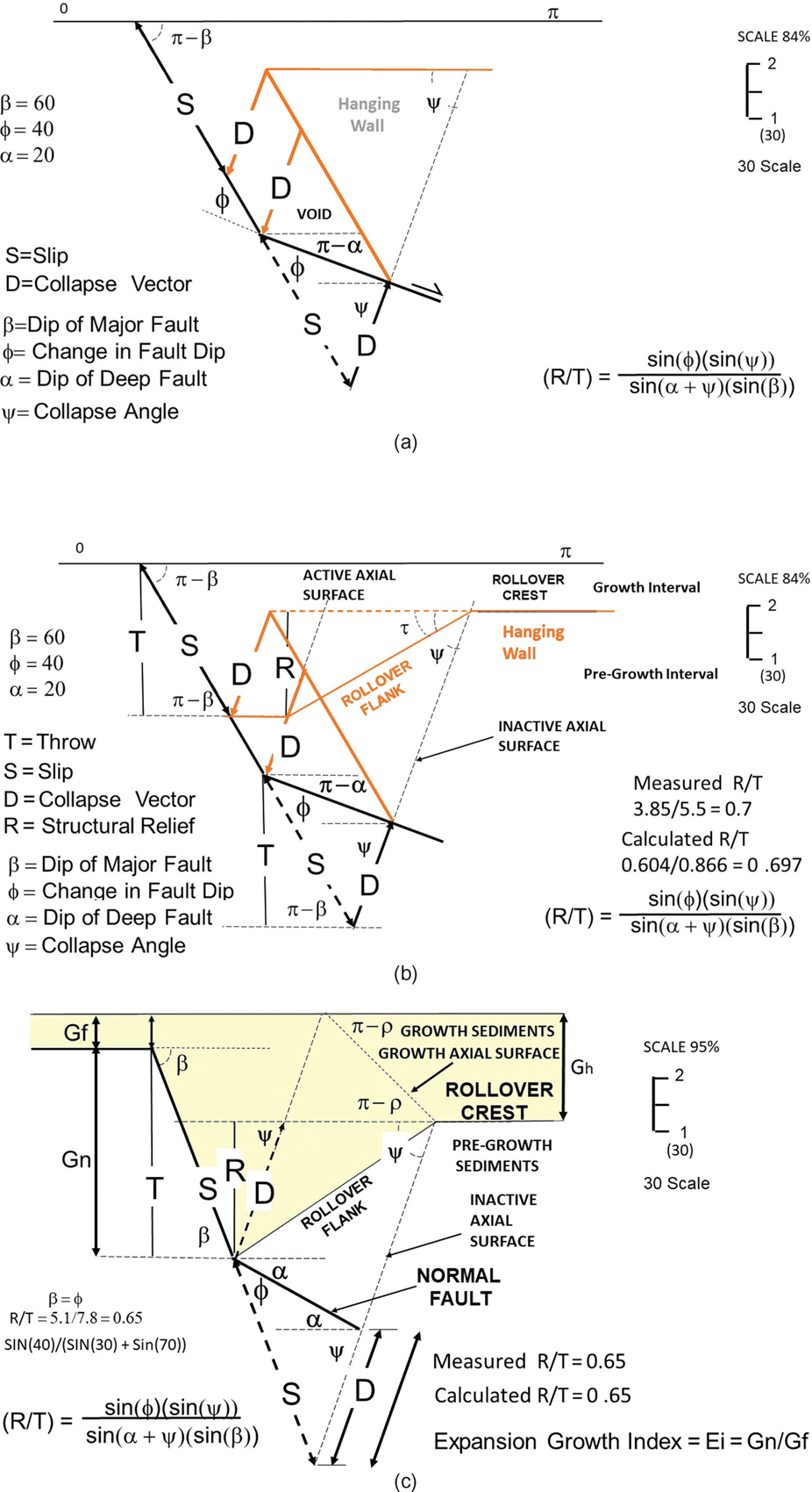
Figure 11-39 (a) Following Hamblin (1965), the hanging wall (colored orange) slips an amount S along the fault surface, creating a void. This void collapses an amount D onto the footwall, generating a rollover structure. (b) The resultant rollover has a structural relief (R) and a throw (T), and thus an R/T ratio can be measured and calculated. This graphic representation shows how the projection of the dashed line S vector beneath the fault bend and the addition of the collapse vector D along the collapse vector (ψ) determines the position of the master fault below the bend. Thus, (b) geometrically defines the ϕ and α angles for pregrowth structures. As the amount of slip increases, the throw also increases along with the D vector, which determines the values of the ϕ and α angles. In addition, and employing the angles shown in (b), the law of sines allows for a calculation of the Rn/Tn ratios. (c) The results of Eq. (11-20) when b = ψ. (Published by permission of R. Bischke.)
For the Gulf of Mexico and Indonesia, the Coulomb collapse angles are about 67 deg to 70 deg (Xiao and Suppe 1992; Shaw et al. 1997; Bischke and Tearpock 2003) (see Fig.11-11). The change in fault angle (ϕ) can be obtained from depth-corrected seismic (Tearpock and Bischke 2003) and the expansion index from depth-corrected seismic or well log data. Thus, the basic theory and procedures exist to accurately predict hanging wall rollover geometries from using structural balancing software packages. Nomograms for predicting the shape of the bed dips in the hanging wall structure are presented in Tearpock and Bischke (1991, 2003). Prospectors typically know that the greater the change of the listric fault angle (ϕ), the steeper the bed dips on the flank of the rollover and the greater the structural relief (R) to the crest of the rollover structure (Fig. 11-38).
This section addresses both pregrowth and synsedimentary or growth structures. On pregrowth structures there is a general mathematical relationship between the structural relief (R), the throw (T) on the fault, and the change in fault dip (ϕ) [see Eq. (11-18) in the section Pregrowth Structure and Calculations], or
where K is a different function for pregrowth or for growth faulted structures.
In pregrowth modeled structures, the closed form equation derivations show that the K function is primarily influenced by the change in fault dip angle (ϕ) (see Pregrowth Structure and Calculations). However, other parameters also influence the shape of pregrowth rollover structures, and in general, K is a function of
[Fig. 11-39b; also see Eq. (11-18) in Pregrowth Structure and Calculations], where (β) = the initial or steepest dipping portion of the master fault and (α) = the dip of the deep portion of the fault beneath the crest of the rollover (Fig. 11-38). Except for the Coulomb collapse angle (ψ), the remaining parameters, such as the structural relief (R)/throw (T), can be measured from depth-corrected seismic sections. All calculations apply to the top of the horizons. However, the base of Horizon H1 is the top of Horizon H2.
General Eq. (11-14) may be used to determine the deep rollover structure and stratigraphy of pregrowth horizons, where the fault surface and seismic reflections image but where the seismic resolution may be of poor quality and/or the sequence stratigraphic relationships are uncertain. Thus, the seismic does not need to be perfectly coherent.
On the more common growth or synsedimentary faults, K is a function of
[see Eq. (11-18) in Pregrowth Structure and Calculations], where (ψ) = the Coulomb collapse angle, (ρ) = the growth axial surface (Xiao and Suppe 1992), and (τ) = angle that the rollover limb dips toward the master fault, defined by inflection points located near the crest and base of the limb (Fig. 11-39b or 11-41).
On pregrowth and growth structures, the method and its equation may also be used to check interpretations for consistency and structural validity where structure is complex or where the correlations are uncertain. Again, the seismic section must be depth-corrected. Following Xiao and Suppe (1992), we introduce simple, modeled derived structures to better understand the properties of real models based on seismic data. They classified models into pregrowth structures and growth structures. The pregrowth, or no-growth, structures are simpler than growth structures and are studied first. The application of these models to existing Gulf of Mexico rollover structures follows. At first, the models are simple, approximating curvilinear surfaces as straight lines, and become increasingly complex.
Lastly, real structures are analyzed. Xiao and Suppe (1992) realized that real structures could be modeled with smaller straight-line segments. In fact, real listric fault surfaces are often curved and have multiple active axial surfaces emanating from small bends in the fault surface (Xiao and Suppe 1992).
Linear Growth
Linear or near-linear growth is not always present but can occur when the R/T picks of seismic horizons, when processed in a spreadsheet, generate linear or near-linear regression coefficients in an x/y equation. The PF (see Table 11-1 for definitions) regressions may have high R-square values. More specifically, the variable R and T depth changes at increasing depths, and the depths of the R and T values adjacent to the master fault are modeled by a linear regression equation with high correlation coefficients. These high correlation coefficients of the measured and calculated depths result in a near linear (T/R) versus depth graph (e.g., Fig. 11-40, and see Chapter 13). Linear or near-linear growth is interesting in that linear functions with high R-square calculations are able to make predictions. For example, if the position of sands or a high %TOC horizon exists in the footwall, and these identical beds have not been drilled in the downthrown block, then the approximate depth of the downthrown beds maybe estimated utilizing the near-linear formula.

Figure 11-40 A graph of Rn/Tn values versus the change in the dip (ϕ) of the fault for a 50-deg and a 60-deg dipping master fault. These values are generated from Eq. (11-18). For pregrowth structures, the graph can quickly check R/T values. For example, using this figure, a change in fault dip of ϕ = 40 deg on a fault initially dipping at β = 50 deg yields an Rn/Tn ratio of 0.8. (Published by permission of R. Bischke.)
The correlations were conducted using well log parasequences and on high seismic acoustic impedance contrast data. Of course, the parasequence data had more correlations than the seismic data. The zero crossings on the seismic were not included in order to simplify the interpretation of the seismic profile. It is generally accepted that if random error is not included, then fewer independent variable correlations are required to justify linearity, even as low as 2 to 3 (Warner 2013). Later in the discussion of syntectonic models, we visually explain, using seismic data, how to identify near-linear growth using growth axial surfaces (Fig. 11-39c).
The cause of this linear or near-linear growth is not well studied but may result from uniform sedimentary loading, causing the master fault to generate linear growth. Linear growth was first recognized in paleontological data (Shaw 1964), then in contractional (compressional) setting using seismic, well logs and outcrop data (Suppe et al. 1992; Suppe et al. 1997; and Shaw et al. 2005). The latter case is interesting in that in order to get linear growth, the sediments must flood over the uplifted structure at a steady state. Linear growth was also recognized in extensional well log data, and segments of linear growth exist between some sequence boundaries (Bischke 1994b; Sanchez et al.1997; Chatellier and Porras 2001, 2004) and was also recognized in field studies (Bischke et al. 1999). Linear growth is also confirmed in well log data collected along strike-slip faults (Shaw et al. 1994). When using well logs, the parasequence correlations can be typically determined within less than a meter (several feet), so the growth data graphs have a high degree of accuracy (Bischke 1994b).
Furthermore, linear or near-linear growth is not uncommon and exists in all environments (Tearpock and Bischke 2003) (for examples, see Figures 13-8, 13-9, 13-11, 13-12, 13-14, 13-17, and 13-21). For example, seven parasequences on depth-corrected seismic had an R-square = 0.982. Knowing beforehand from the seven parasequence examples presented above that only one of the examples was linear suggests that linear growth may be more common than realized. Linear growth just exists within sedimentary sequences. We do not suggest that linear growth is always present, as published examples in the preceding references also contain nonlinear sedimentary growth. Despite the evidence of linear or near-linear growth along normal faults, no studies have been published on how linear growth occurs or on its extent. On the other hand, linear growth associated with contractional structures has been subject to numerous studies (see preceding references).
Unlike contractional structures in which the growth sediments must flood over the uplifted structures, as long as the normal fault is slipping, extensional normal faults create accommodation space to trap growth sediments. It is important to understand that growth measurements involve thickness changes and are not directly related to time (Suppe et al.1992). Unlike growth sedimentation, empirical determinations of sedimentation rates are known to scale—or obey fractal mathematical relationships, which plot as a negative sloping power law on a log/log scale (Sadler 1999). In other words, mean sedimentation rates are high over short time periods, and sedimentation rates are smaller over long time periods. In effect, longer time periods allow for more and/or larger hiatus, which include nondeposition or erosion (Sadler 1999). The important point is that sedimentation rates are strongly dependent on the time frame of reference.
Industry acknowledges that thin growth sections on normal faults (let us assume a growth section of 100 feet, or 33 m) were deposited over shorter time frames than growth sections measuring several miles thick (assume 2 miles, or 3.2 km) (for extensional examples, see Tearpock and Bischke 2003; for contractional examples, see Echavarria et al. 2003). Thus, in analogy with sedimentary rate data, thin growth sections are unlikely to contain many large or numerous hiatus (sequence boundaries, unconformities, or erosion), while thick growth sections are likely to contain more and larger hiatus. We are not familiar with any study that addresses these issues for normally faulted sections.
Calculations and Examples
This section shows how to calculate and describe equations for pregrowth and growth structures. Pregrowth structures are discussed first. The following pregrowth and growth models contain both measured and calculated values (see definitions described in the next section, Measured and Calculated Values on Graphs). Only the most salient aspects of rollover formation are reviewed, and the details of rollover formation are covered by Xiao and Suppe (1992) and in the first five sections of Chapter 11 in Tearpock and Bischke (2003).
Pregrowth Structure and Calculations.
Rolled-over beds (hanging wall anticlines) are caused by a void that develops between the hanging wall and foot wall of a normal fault, as the hanging wall beds slip (S) along the footwall fault surface (Hamblin 1965) (Fig. 11-39a). The weight of the hanging wall instantaneously closes the void caused by Coulomb shear collapse (ψ). The shear, which parallels the collapse angle, produces the rolled-over bed geometry (Hamblin 1965; Xiao and Suppe 1992) (Fig.11-39b).
In Figure 11-39b, the amount of the collapse required to fill the void is shown by the vector D, which parallels the collapse angle (ψ). In other words, the magnitude of vector D represents the amount of displacement required to cause the hanging wall to collapse onto the footwall (Hamblin 1965), closing the void. This collapse process forms the flank of the rollover, which dips toward the fault between the active and inactive axial surfaces and forms the structural relief (R) (Fig. 11-39b). The vector D is the vector Ax in Xiao and Suppe (1992). The structural relief is defined by the inflection points on the flank of the structure. The vector D vector is determined by the amount of slip (S) or throw (T), the Coulomb collapse angle (ψ), the change in dip (ϕ), and the dip of the fault (α) at depth as the hanging wall moves over the footwall (Fig. 11-39b). (Consult Table 11-1 for the definition of symbols.)
A graphical or inverse model solution to the structure consists of several steps. First, a copy of the modeled hanging wall is constructed from the fault surface, and the hanging wall slips over the footwall. Next, parallel to the dip of the shallow portion of the fault surface (β), project the amount of slip (S) below the bend in the major fault surface. Then, parallel to the inactive axial surface, add the D vector to the tip of the slip vector (S) (Fig. 11-39b). The D vector determines the position of the deep fault surface (α) and also determines the flank dip angle (τ) of the rollover.
Using the law of sines, a mathematical solution from Figure 11-39b is as follows:
where
where

Substituting Eqs. (11-16) and (11-17) into Eq. (11-15) and employing trigonometric identities eliminates π from Eqs. (11-15) and (11-16), and all of the angles are first-quadrant angles. This formulation yields
and rearranging yields
or
If ψ = β, then Eq. (11-18) simplifies to
where
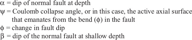
Equation (11-22) yields the Rn values if the Tn values are measured. Equation (11-20) is plausible, as the major fault dip (β) could initiate or fracture at a 67-deg to 70-deg angle, or for dips approximating the Coulomb collapse angle ψ [see Fig. 11-39c to calculate R/T for Eq. (11-20)]. A study of the shallow portions of large expansion faults using depth-corrected data had a range of values between 60 and 45 deg for β. Figure 11-40 was created using Eq. (11-18) for Figures 11-39b and 11-41, assuming 50-deg and 60-deg angles for β, α = 20 deg, and ϕ = 40 deg. Even with four sine equations, the results are nearly linear. The accuracy of Figure 11-40 can be checked against Figures 11-39b and 11-41. In addition, from depth-corrected data and knowing the footwall stratigraphy and fault shapes, from well control or seismic data, Eq. (11-18) can be used to predict the throw or structural relief across large pregrowth faults and thus the downthrown stratigraphy (Fig. 11-41).
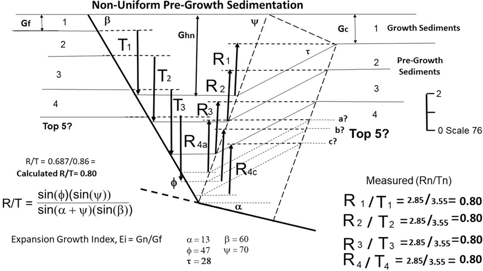
Figure 11-41 A simple modeled pregrowth structure that exhibits uniform sedimentation in the hanging wall and footwall for horizons H1 to H4. The amount of throw (Tn) and structural relief (Rn) vectors are shown for each horizon. Unlike growth structures, pregrowth structures dip in a uniform horizontal width toward the largest bend (ϕ) in the normal fault. Hand-measured values of Rn/Tn are posted on the figure along with the calculated value from Eq. (11-18), and the definition of the expansion index (Ei). Horizon 5 is assumed to be in a poor data area, but its hanging wall depth can be predicted by the Rn/Tn plot proposed in this study. (Published by permission of R. Bischke.)
A Pregrowth Structure
A pregrowth structure (Fig. 11-41) is distinguished from a growth structure in that the rolled-over beds form a band or dip domain of uniform horizontal width that typically converges toward a large bend in the listric fault. However, if the growth is a syntectonic or growth fault and the growth increases with depth, then the growth-faulted rolled-over beds grow wider with increasing depth (Xiao and Suppe 1992) (Figs. 11-38 and 11-44). In Figure 11-39b, notice that the bed is rolled over at the bend in the fault surface (ϕ). The active axial surface emanates from this bend and dips at angle of about 67 deg. The (ψ) surface is active as shear along the (ψ) surface propagates into the hanging wall and defines where the beds roll over (Xiao and Suppe 1992).
In the hanging wall, the vertical distance between the top, or crest, of the structure and the depth at which the dipping beds are near horizontal defines the structural relief (Rn). Let us assume in Figure 11-41 that (1) sands are present in the footwall at the top of horizon 5, (2) in the hanging wall and in the vicinity of horizon 5, the data are semicoherent and cannot be correlated from the hanging wall into the footwall using reflection character, and (3) all of the wells in the hanging wall penetrate only as deep as horizon 4. Which is the correct solution to the depth of horizon 5? To determine the correct horizon, geoscientists can measure the Rn/Tn ratios for horizons 5a, 5b, or 5c (Fig. 11-42).

Figure 11-42 A structural relief(Rn)/throw(Tn) versus depth(Zn) plot for the uniform R/T data posted on Figure 11-41. The top of horizons H2 to H5b have the same R-square value of 1.0. From this figure, horizon 5 has a unique depth(Zn) value of 9.05 units. Horizons H5a and H5c represent potential miscorrelations. (Published by permission of R. Bischke.)
A convenient way of illustrating the correct horizon position—5a, 5b, or 5c—is by projection and then displaying the Rn/Tn results on an Rn/Tn versus depth(Zn) plot (Fig. 11-42). Depth(Zn) is the total depth to the base of the Rn/Tn or Hn values, typically the subsea depths to the horizons or to a datum below the surface. These plots have been called Δd/d or throw (T) versus depth (Z) plots in the literature (Bischke 1994b; Pochat et al. 2004). Again, depth(Zn) is the total depths to the base of the throw(Tn) and structural relief(Rn) vectors. When applied to well log data, these plots have an accuracy of better than 5 ft/10,000 ft, or a 0.05% error, at a depth of 10,000 ft (3049 m) (Bischke 1994b). Seismic resolution accuracy at this depth is substantially lower than well log data (Sheriff 1980), and thus the error is higher. Geoscientists can determine seismic resolution from vertical Fresnel zone nomograms that are a function of frequency, that decreases with depth, velocity, and wavelength (Sheriff 1980).
Figure 11-42 is a Δd/d or structural relief(Rn)/throw(Tn) versus depth(Zn) graph for the measured data in Figure 11-41. Also, note that the base of Horizon H1 is the top of Horizon H2. Projecting the base of horizons H1 to H4 and the R2/T2 to R5/T5 data and to depth leads to the obvious conclusion that the Horizon H5b data point on the graph is the correct answer. Notice that the H5b horizon R5/T5 data matches Rn/Tn data for the top of horizons H2, H3, and H4. Also, notice that the R5b/T5b data point has a unique depth(Zn) position on the graph of 9.05 units (Fig. 11-42). This follows, as the Rn/Tn measurements for the top of horizons H2 to 5b all have the same values of Rn/Tn = 0.80 (Figs. 11-41 and 11-42). The Rn-square or FP correlation values (see Table 11-1 for definition) for these horizons is 1.0. This makes sense, as the pregrowth sequence was deposited prior to the faulting and the faulting is post-depositional (the Tn values in Fig. 11-41 all have the same value). Thus, all of the horizons must have the same throw(Tn) values, in this case equal to 3.55 units. A plot of the throw(Tn) values versus depth(Zn) would confirm these conclusions. The calculated Rn/Tn value is 0.80, which is calculated from Eq. (11-18).
Figure 11-40 is a Rn/Tn versus depth(Zn) graph, which has properties similar to those of Δd/d plots in that outlying points constitute an anomaly. The cause of an anomalous point must be investigated, and this technique is discussed in detail in Chapter 13. The possibility that the horizon points H5a and H5c are the result of variable geology are unlikely. This conclusion follows, as the horizons were continuous when deposited and were deposited in a near horizontal position prior to the faulting. Excluding the possibility of a channel, stratigraphy does not change across a nonexistent fault. The possibility of a channel can be checked on adjoining lines. A possible but less likely explanation is that a major unconformity terminates by coincidence at the fault surface. Again, this explanation is unlikely, as the nonexistent fault was not moving and could not represent a buttress to onlapping sediments. Also, adjacent lines may resolve this possibility. Another option is to create a figure similar to Figure 11-42 using different depth(Z) values, such as points H5a and H5c, which do not match shallower Rn/Tn = 0.8. If the problem is an improper depth correction and a velocity error, then the velocities can be checked and the graph will help correct the incorrect velocities to a proper value. The correct depth will correspond to the depth in which Rn/Tn = 0.8. Lastly, another option exists when confronted with an anomalous situation in which it is not possible to correlate from the footwall into the hanging wall using seismic reflection character. In pregrowth structures, as the hanging wall along the fault surface must fit back into the footwall, structural balancing or, more specifically, retrodeformation may help (see Chapter 10, Fig. 10-10).
The next plot (Fig. 11-43) is based on Figure 11-41 and contains a deep single bend (ϕ) below Horizon H5. As the beds have not moved through the bend in the fault, the data points shown in Figure 11-43 are impossible in uniform thickness pregrowth strata, as the downthrown and upthrown beds must have the same thicknesses and thus the same Rn/Tn values. This interpretation of the data is possible as a result of poor seismic data or poor stratigraphic correlations. The Rn/Tn versus depth(Zn) graph (Fig. 11-43) looks reasonable except for the FP calculation of 0.357. In addition to the low FP value, the Rn/Tn plot in Figure 11-43 looks more random than the data in Figure 11-42. Assuming that the best linear fit is the most probable answer, possible problems exist in horizon correlations H4 and H5. These horizons appear more anomalous than correlations H2 and H3, which could be better. If there are any questions as to data anomalies, the following ratios can be graphed. Ratios, such as Rn/Tn ratios, are more sensitive than direct depth measurements such as the throw (T), which in this case, because the faulting is post-depositional, has a uniform value of 3.55 units (Fig. 11-41).

Figure 11-43 Nonuniform sedimentation between the hanging wall and footwall cannot exist in pregrowth structures. This follows, as the marine sediments are typically deposited at low dip angles, and the faulting is post-depositional. The low linear regression R-squared result of 0.357 indicates that there is a problem with the interpretation. (Published by permission of R. Bischke.)
Accuracy of Methods
One way to address accuracy or correctness is to calculate the FP and R-squares of the data. Another is to calculate the % differences of the data. Percentage differences have the property that the order of the numbers do not matter. The % difference takes the averaged sum of the largest and smallest horizon thicknesses (Gn) (Fig. 11-44), then divides this number into the horizon thickness differences between the largest value minus the smallest value multiplied by 100. As there are no horizon thickness differences in the correct values measured on Figure 11-42, the % difference = 0.0, which means that the data have zero variations. The following discussion on growth and real structures contains % differences that are much larger. Large % differences can affect the accuracy of any projection method, but methods exist to recognize, address, and mitigate large % differences in real structures. (See Fig. 11-45 for the general equation).

Figure 11-44 Figure used to calculate growth formula for variable sedimentation. The M1, N1 portions of the triangle are colored in orange, and the law of sines formulation for growth structures is shown for the M1 and N1 vectors on the right side of the figure [Eq. (11-28)]. For clarity, the rounded measured and calculated values for the M1–N1 to M4–N4 vectors are posted on the left side of figure. (Published by permission of R. Bischke.)
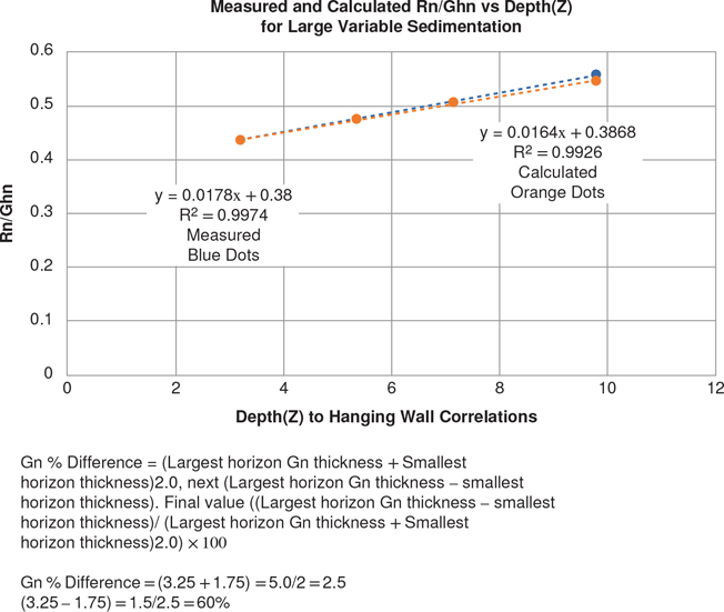
Figure 11-45 A Rn/Ghn plot versus total depth(Zn) for the Figure 11-44. The measured and calculated values for variable sedimentation show near-linear growth. The % difference values are high with a 60% variation. Thus, the R-squared result for the measured values is 0.997, but the calculated result is only near linear at 0.993. (Published by permission of R. Bischke.)
The calculated values for graphs use Eqs. (11-18) and (11-28) to (11-30), and the measured values often used higher-imaged scales (200% to 400%), a magnifier, and typically a 30 scale (1/30 of an inch). Thus, the measured values have errors of up to 0.0167 in. = (1/(30 × 2) = (0.042 cm) (the viewing scale is shown as a percentage above the measured scale at 1/60 inches).
Growth Structure and Calculations
Figure 11-44 shows a modeled growth structure labeled to calculate growth on a simple fault (0 is on the left, and π is on the right). Measurements are taken from the horizontal, and ρ can exceed 90 deg, but in the formula π − ρ is less than 90 deg. As described in the section Details for Constructing Triangles, the object of the following calculations is to create a triangle often, but not always, bounded by an axial surface dip ψ. In this case, the triangle is formed by the vector Mn, flank dip vector Nn, and ρn (see Fig. 11-44).
Down to the Right Faults
The following formula is for a down to the right fault, or one that flattens to the right. Thus, if by convention, 0 is next to the shallow portion of the master fault, and π is above the deeper portion, then down to the right faults satisfy Eq. (11-28) (see Table 11-1 for definitions of terms). In this case, for (ρn > ψ) and from the law of sines and Figure 11-44,
where
where, as before, R1 is the structural relief for Horizon H1, but (T1 + Gf) is the throw plus the sum of the growth section from the base of the horizon being calculated to some datum located at or below the sea floor (Fig. 11-62a). Similarly, Gh1 is the total sedimentary or growth section for the horizon being studied to a datum, which in this case is from the base to the top of Horizon H1 (Fig. 11-44).
Substituting Eqs. (11-24) and (11-25) into Eq. (11-23) yields
However, in general and as the horizon deepens and the flank dip often increases, the total Depth(Zn) of the base of Horizon Hn increases and thus, in general, from Figure 11-44,
where
n = 2, 3, 4, . . . m for top of Horizon Hn
ψ = Coulomb shear collapse angle, typically 67 to 70 deg
ρn = dip of the growth axial surface in Figure 11-44, which in this case is the angle π–ρ
τn = frontal dip of the rollover structure defined from inflection points, located near the crest and base of structure for the top of Horizon Hn
Ghn = total thickness of growth sediments for the base of Horizon Hn (which has a thickness Gn), which is equal to the total depth(Zn) of the horizon being studied. The Ghn depth is taken relative to a datum depth that can exist below the surface or sea floor. The chosen datum can affect the accuracy of Eq. (11-28).
One exception to Eq. (11-28) is that in multibend or nonlinear structures, if the right side of the triangle is not ρn and is replaced by ρm, where m = a, b, c, . . .z, then, Eq. (11-28) becomes
(See sections The Growth Axial Surface Increases Dip and The Growth Axial Surface Decreases.)
Formula for Down to the Left Faults.
This equation follows the same formulation as Eq. (11-28), and its derivation is also
but with 0 on the right.
Accuracy of Eqs. (11-28), (11-29), and (11-30).
Sine functions can be sensitive, and the datum can be adjusted to more stable angles. The ψ, or the Coulomb collapse angle, is a constant, and the dip of the limb dip (τ n) range is not as large as the ρn angle range. Thus, the calculation accuracy of Eqs. (11-28) to (11-30) is mainly dependent on ρn. If the ρn − ψ dip angles are less than about 5 to 10 degrees, then if possible, use a datum that results in ρn − ψ angles that are between about 45 to 130 degrees. This procedure will result in lower calculated ρn − ψ errors and thus in better Rn/Ghn values.
Details for Constructing Triangles.
In Figure 11-44, vector M1, which is an active axial surface ψ for Horizon H1, the growth axial surface ρ1, and the dip of the flank N1 form a triangle. Vector M1 in Eq. (11-25) defines Gh1/sin(ψ). Also, N1 = R1/sin(τ 1) [Eq. (11-24)]. As long as the growth axial surface, ρn, and Nn values do not change dip, the angles do not change. According to the general Eq. (11-28), R3/Gh3 is defined by angle (ρ − ψ), and length of vectors M3 and N3 (line N3 dips at τ 3 degrees) (Fig. 11-44). It is important to remember that when the horizons or the growth axial surface (ρn) changes dip, the calculations require the formation of new triangles, with new angles for each horizon studied. In this case, the τ 1 angle dips more gently at the crest of Horizon H2, and the dip increases with increasing depth.
When analyzing a seismic line, geoscientists can predict whether the depth-corrected structure is near linear by observing the dip of the growth axial surface ρ. If ρ appears to be near linear, then the calculated and measured data points are likely to generate a near-linear line when processed by a linear regression option in a spreadsheet. Thus, along some seismic lines a straight line, or a nearly straight line ρ, can be drawn on the seismic line at the crest of structure (red lines on Fig. 11-62a). The ρ lines, although not directly entered into the equations, are part of the visual data.
As before, Rn is the structural relief, and Ghn includes the total thickness of growth sediments for Horizon Hn to a datum located at or below the sea floor as described previously. Figure 11-44 is a high-growth rollover type of model resulting from changing Ghn and Gn thicknesses, and changes in the frontal rollover dip angles τn. The changing τn dip values could be caused by sedimentary onlap. The variable sedimentation Rn/Ghn plot (Fig. 11-45), generated from Figure 11-44 data, nevertheless exhibits a near-linear calculated and measured growth versus depth plot. Every point on the plot on Figure 11-45 represents a new formula formed by new values in the equation. On this plot, the Gn % difference is 60%. Calculated values, using Eq. (11-28) may generate larger R-square values than measured values, but not always. PF coefficients (see Table 11-1 for definition) typically get better at lower % differences calculations ranging from below about a 50% to 70% difference. Thus, R-square variations reflect the linearity of the equations.
Measured and Calculated Values on Graphs.
For measured values, the figures were made larger at a scale of 200% to 400%, and the Rn/Tn values are measured directly with a scale ruler and a magnifying glass, resulting in a measurement error of about 1/60. For syntectonic structures, defined by Eqs. (11-28) to (11-30), the calculated and measured values are compared to each other on the graphs. The posted calculated values on all of the graphs use angular measurements defined from the right-hand side of Eqs. (11-28) to (11-30) (calculated values on Fig. 11-45). Notice that from the left-hand side of Eqs. (11-28) to (11-30) is the ratio
This ratio is measurable. Thus, the measured values for Eq. (11-31) are first obtained by measuring the lengths of Rn and Ghn. The left-hand side of Eqs. (11-28) to (11-30) is then determined from Eq. (11-31) by dividing Rn by the measured value of the total growth (Ghn), or depth(Zn), from a chosen datum to the horizons being studied. The Ghn = depth(Zn) values are much larger than the Rn values.
Syndepositional Growth Models
In nature, syndepositional growth structure is more common than pregrowth structure and is structurally more complex. For example, geoscientists have recorded growth on normal faults using expansion indices (Thorsen 1963) or throw (Tn) versus depth(Zn) diagrams (Bischke 1994b; Sanchez et al. 1997; Tearpock and Bischke 2003). Expansion indices (Ei) typically compare downthrown horizon or sequence package thicknesses (Gn) divided by the equivalent upthrown sequence thicknesses, here defined as Gn/Gfn (see Fig. 11-46 for the definition of depth(Zn) and Gn/Gf). An alternative is to correlate thickness on the crest of the rollover structure to upthrown thicknesses, here defined as Gc/Gf (Fig. 11-46, right-hand side). If the growth is roughly uniform, then Eq. (11-18) in the Pregrowth Structure and Calculations section can be used to confirm the correlations. If the growth axial surface changes rapidly, then Eq. (11-28) is modified to correct for the change in growth (Fig. 11-52).
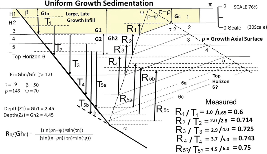
Figure 11-46 This figure is a growth or syndepositional structure that exhibits uniform growth. On growth structures, the throw(Tn) and structural relief(Rn) values increase with depth as the limb of the structure widens with increasing depth(Zn). Accordingly, the Rn/Tn values also increase with increasing depth. The equation on the figure is the growth equation for a uniform growth axial surface (ρ). (Published by permission of R. Bischke.)
This discussion starts with the simplest models first, by developing models that have uniform or a small amount of growth. For this low-growth analysis, the late and rapidly growing sediments infilling the most recently deposited sediments are not included in any calculation. For example, if the thickness of Gf is about 0.0 in the models, then the expansion index calculations Gn/Gf would be near infinite, making the % difference evaluations useless. Thus, Horizon H1 (Fig. 11-46) will be included only when investigating large-growth sedimentation models. The initial models will concentrate on simple uniform growth. These models have a straight-line growth axial surface (ρ) (Xiao and Suppe 1992) and where no variations in sedimentary thicknesses exist. This assumption permits for a simple understanding of the methods, which are then made more realistic. Typically, lower R-square values indicate a more complex model, and thus R-square values are reported in the text. Understand that the R-square values reflect the correlation calculations!
Uniform Growth
In the simple uniform sedimentation model (Fig. 11-46), the measurements and calculations start at the top of Horizon H2. In this model, the downthrown stratigraphic horizon thicknesses do not change, and the growth and corresponding Rn/Tn measurements are linear. The geometry of syndepositional structures expand, and the horizontal width of the structure grows wider with depth. The growth axial surface (ρ) defines the top or crest of structure (Xiao and Suppe 1992) and is a constant in this model (Fig. 11-46). If (ρ) appears to be linear, as in Figure 11-46, then the linear regression results will exhibit high R-square values, and the growth will be linear. This occurs in real or modeled data. If the growth axial surface does not change dip, and the horizons (Gn) do not change thickness, then the expansion index Gn/Gf does not change and the growth is uniform. Again, the vertical distance between the top, or crest, of the structure and its flank, which is the depth at which the beds no longer dip, define the structural relief (Rn). Thus, R1 is the vertical distance between a horizontal line drawn at the crest of structure (that terminates at the position of the growth axial surface) and a point on the flank of the structure where the horizon is roughly horizontal. Again, we assume that the position of the top of Horizon H6 is not clearly known (Fig. 11-46).
Figures 11-47a and b are an Rn/Tn and Rn/Ghn versus depth(Zn) plot. The mathematical formulation of expansion faults is covered in the Pregrowth Structure and Calculations section. Notice that the Rn/Ghn plot (Fig. 11-47b) does not require footwall data, as Ghn exists only in the hanging wall. The measured structural relief(Rn)/throw(Tn) and calculated Rn/Ghn values are near linear with an R-square very close to 1. Measurement errors are the cause of the imperfections. The misinterpreted horizons 6a and 6c clearly deviate from the more linear trend on Figure 11-47a. Ratios, such as Rn/Tn versus depth(Zn) graphs, are more sensitive than direct measurements of Rn and Tn, both of which can contain minor errors. Studies of the models generally show that the structural relief(Rn) versus depth(Zn) graphs tend to have the highest R-square results from the linear regression. Figure 11-47b contains the same data plotted in Figure 11-46, but the data are calculated using Eq. (11-16) and angles. Growth measurements (Ghn) is always measured from the datum for horizon Gn to the base of the horizon being studied [Fig.11-50 and Eq. (11-13)]. In this data set, the direct measurements result in an R-squared of 0.9919 (Fig. 11-47a). The calculated data from Eq. (11-18) result in an R-squared = 1.0 (Fig. 11-47b). The result is constant, as the angles do not change between horizons. The measured values result in an R-square of 0.9, which results from direct measurement errors (consult Measured and Calculated Values on Graphs for definitions of measured versus calculated values). Data with a positive slope on these Rn/Tn diagrams means that the structure is growing larger with depth(Zn). As a result of this growth, the sedimentary wedge grows thicker. On Figure 11-47a, the total depth to the top of horizon 6b is 10.3 units. The position of the R5/T5/base depth(Z5) (which defines the top of horizon 6) value has a unique position on the linear, calculated uniform growth graphs (see the Gh1 = 2.45 and Ghn = 4.45 calculated depths on Figure 11-46). Thus, by projection, the top of Horizon H6b is the correct horizon top for uniform growth, and not horizons H6a or H6c.The data set need not be perfectly linear to conduct this projection exercise. An R-square near or at 1.0 means a high correlation is involved in the projection process.
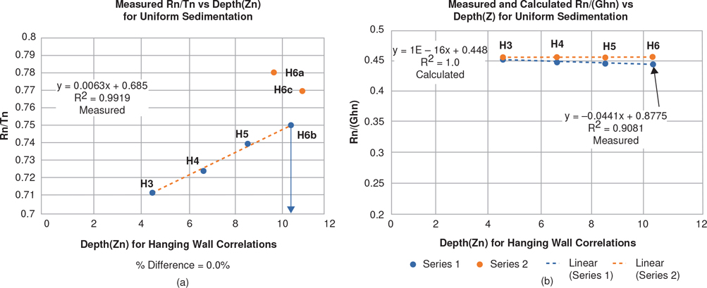
Figure 11-47 (a) The measured Rn/Tn values are linear correlation for horizons H3 to H6b and have a high R-squared value. The depth(Zn) value is measured from the base of Horizon Hn to the top of the growth. (b) The measured Rn/Ghn values are not as accurate, which is not typical. However, the calculated linear regression R-squared results, using Eq. (11-28), are 1.0 for H3 to H6b. (Published by permission of R. Bischke.)
In normally faulted structures, delta (Δd)/d (change in depth/depth) plots of stratigraphic sequences are also often near linear, indicating near-linear stratigraphic growth within sedimentary sequences (Bischke 1994b; Sanchez et al. 1997; and Bischke et al. 2006). Thus, near-linear growth is not uncommon (Tearpock and Bischke 2003) (Figs. 13-8, 13-9, 13-11, 13-12 13-14, 13-17, and 13-21).
The graph represented in Figure 11-48 is similar to the graph shown in Figure 11-46, except that the displacements are larger and horizons H7, H8, and H9 have moved through the active axial surface into an inactive zone. In this case, these horizons have moved through the bend in the fault bend defined by (ϕ), and these horizons dip onto the deep portion of the fault defined by α (Fig. 11-46). Notice that the calculations for throw(Tn) on Figure 11-48 for horizons H7 to H9 do not change and have the same values. The constant values mean that the region to the right of the active axial surface is inactive and lacks any deformation.
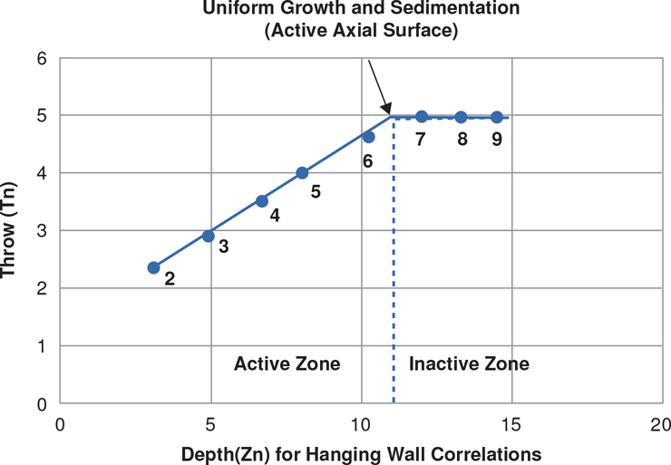
Figure 11-48 This model is very similar to the model shown in Figure 11-46, but the strata pass through the active axial surface into the inactive zone to the right of the active axial surface. No deformation occurs in the inactive zone. (Published by permission of R. Bischke.)
Low Variances in Growth Sedimentation
Similarly, if the sedimentation differences have relatively low slopes, then the growth plots are nearly linear (Fig. 11-49) and are similar to Figure 11-47a. As the growth approximates uniform growth, the calculated Rn/Tn values have an R-square = 0.99, and thus this model, like the previous model, is relatively simple. Hereafter both the growth and sedimentation variances are posted on Figure 11-49 and on all of the remaining higher-growth figures. The following discussion on growth contains % differences that are much larger than low-growth sedimentation differences.
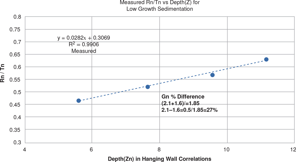
Figure 11-49 If the growth does not vary significantly, the results are similar to uniform growth, but the % differences in this low-growth model increase to 27%. (Published by permission of R. Bischke.)
The Rn or Tn % differences have no meaning on growth structures, as the Rn or Tn values often increase and have a larger value with increasing depth(Zn). However, the horizon thicknesses Gn or the Ghn/Gfn values can define differences in sedimentation thicknesses that affect growth and its linearity. Thus, Gn % differences will define sedimentation variations on growth structures. On Figure 11-49, the Gn % differences have a 27% variation.
High Variations in Growth
Thorsen (1963) showed from correlations of well log data that expansion index Ghn/Gfn defined displacements on listric growth faults. The growth typically increases with increasing depth, reaches a maximum, and then decreases (Fig. 13-3). Thus, growth on listric faults is typically not random. Nevertheless, we test a nonuniform, or random, sedimentation model on a relatively high horizon thickness Gn, hanging wall % difference data (Figs. 11-50 and 11-51a and b) scenario. As a result of the large % difference values of 113%, the Rn/Tn data are less reliable with a measured R-square of 0.9335 (Fig. 11-51a) that indicates lower correlations, but this R-square value could indicate a less certain interpretation.
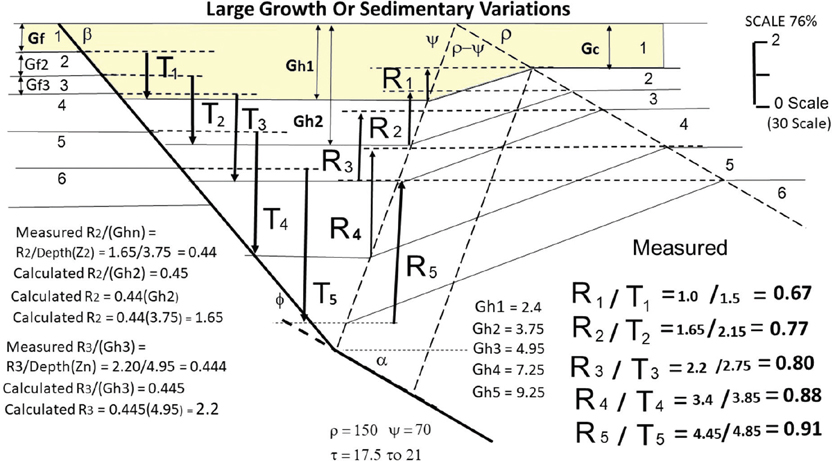
Figure 11-50 A model showing nonuniform growth sedimentation, which is not typical of many structures. Measured and calculated values for horizons H3 and H4 (R2/Gh2 and R3/Gh3) are posted on the left-hand side of the figure. (Published by permission of R. Bischke.)
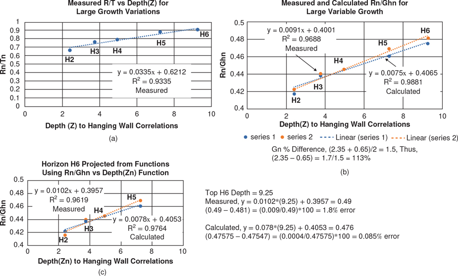
Figure 11-51 (a) As a result of more random sedimentation, the measured Rn/Tn data are less reliable and have a lower R-squared than more uniform growth. (b) However, the calculated data using Eq. (11-28) is more reliable with a linear regression result of R-square 0.988. When the % difference is around 50% to 70% or greater, with the exception of increasing growth, the linear projection assumption maybe less reliable. (c) Test of the projection method assuming that the location of the top of Horizon H6 is unknown. Measured and calculated R6/Gh6 values are shown along with the relative errors. (Published by permission of R. Bischke.)
However, the calculated Rn/Ghn plot (Fig. 11-51b) is near linear with a correlated R-square result = 0.988 even though the Gn % difference variance is 113%. When the % difference data exceed about 50% to 70%, the correlation of the data may or may not significantly decrease. Also, posted on Figure 11-50 are the rounded measured and calculated values for R2/Gh2 and R2/Gh3 and the Rn/Tn values. (See Measured and Calculated Values on Graphs for the definition of calculated and measured values).
Figure 11-51c tests the accuracy of the correlation, projection method assuming that the position of the top of Horizon H6 is unknown. This is accomplished by excluding Horizon H6 data from the data set and using only the H2 to H5 data on the plot. The recalculated Rn/Ghn values are shown in Figure 11-51c (notice that a comparison of Fig. 11-51b and c show slight differences in the y, Rn/Ghn, and R-square values). Thus, it is possible to predict the top Horizon H6 by evaluating the two y/x equations in Figure 11-51c. Simply insert the x = depth value for the top of Horizon H6, which is 9.25, into the two equations (Fig. 11-51c). The measured and calculated solutions are 0.49 and 0.476 respectively. Next, the relative % errors can be determined from the results of the two plots by (1) taking the measured and calculated values from Figure 11-51b, then (2) subtracting the values from the Figure 11-51c results, and (3) determining the % relative error by multiplying the difference by 100. The measured and calculated relative % errors are 1.8% and 0.085% respectively (Fig. 11-51c).
The Growth Axial Surface Increases Dip
In the modeled examples described, the growth axial surface remains constant. Figure 11-52 shows an example of the growth axial surface changing dip and dipping at a lower angle, thus increasing the growth-angle (ρ1) dips at 139 deg and then dips at ρ2 = 153 deg at greater depths. In Eq. (11-28), the ρ1 and ρ2 angles are subtracted from (ψ) = 70 deg. Thus, there are two sources of changing growth in Figure 11-52: the change in the horizon thicknesses and the change in the dip of the growth axial surface. A more gently dipping growth axial surface means that the growth decreases (Xiao and Suppe 1992). On seismic sections, this change in the growth axial surface is recognized by a shift in the position of the crest and flank of the rollover structure. In this case, the crest of the rollover shifts to the right. If, however, the growth increases, then the growth axial surface bends downward, and the crest of the structure narrows and shifts to the left (Fig. 11-54). Furthermore, this change in growth creates a discontinuity in the data (Fig. 11-53a), indicating that the problem is nonlinear. This nonlinearity must be adjusted for in the measurements and calculations. Typically, solutions to nonlinear problems are not trivial.
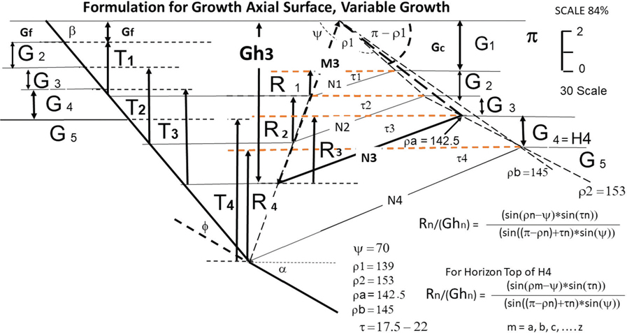
Figure 11-52 As the growth axial surface (ρn) changes, the problem is nonlinear. (Published by permission of R. Bischke.)
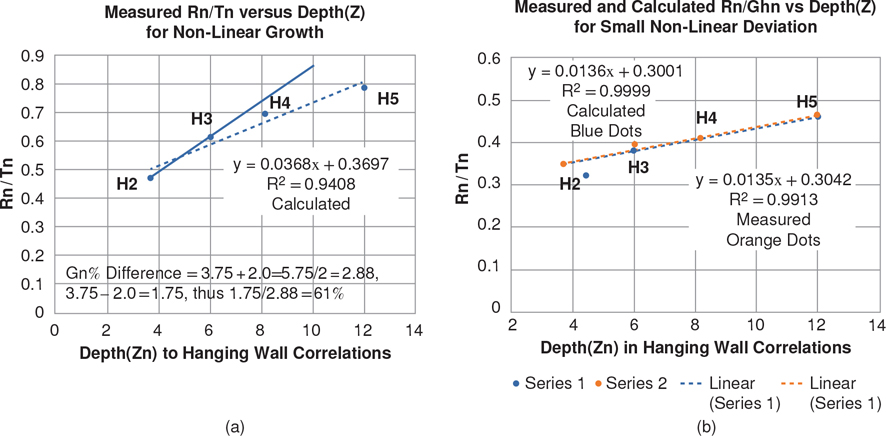
Figure 11-53 (a) The large changes in growth on nonlinear structures cause the Rn/Tn values to have a lower R-square value of 0.94. The high Gn % difference = 61% results in a lower R-square result. (b) However, the values for the calculated linear regression results are R-square = 0.999 and 0.99 for the measured Rn/Ghn values. (Published by permission of R. Bischke.)

Figure 11-54 A growth model, modified from Figure 11-52. Steeply dipping growth axial surfaces may image on seismic, and in this model decrease from ρ1 = 139 to ρ2 = 130 deg; if recognized on seismic, decreasing growth can be corrected on the Rn/Tn and Rn/Ghn plots (Fig. 11-55a and b). (Published by permission of R. Bischke.)
This topic is also briefly discussed in the Pregrowth Structure and Calculations section, where a detailed derivation of Eq. (11-18) is presented. The following is a description of how to calculate the right-hand side of Eq. (11-28) to adjust for nonlinearity. Notice on Figure 11-52 that the growth axial surface (ρ1) for the crest of horizons H1 and H2 does not change position. Thus, (ρ1) does not change in the calculations for the first two horizons. The solution for the top of Horizon H3 in Eq. (11-28) is to form a triangle that includes the angles (ρ1), ψ, and the value of the bed dip τ2 [use radians in Eq. (11-28) for a computer-generated solution].
At the crest of Horizon H4 (or the bottom of Horizon G3), the growth axial surface abruptly changes dip from ρ1 = 139 to ρ2 = 153 deg, and this change in the growth axial surface shifts the position of the crests of horizons H4 and H5 to the right. In order to adjust for this nonlinear behavior, the triangle formed does not include the growth axial surface (ρ2) but rather the angle ρa = 142.5 deg. Thus, in Eq. (11-28), the ρm replaces the angle ρn, and Eq. (11-29) contains the term ρm − ψ in the numerator (consult Fig. 11-52 for variable ρ values). The lengths M3 and N3 and the angle ρa = 142.5 deg are shown in bold on Figure 11-52. Also, notice that for the base of Horizon H4, the value of the growth axial surface changes to ρb = 145 deg, both N4 and M4 lengthen, and τ4 increases. This change must also be incorporated into Eq. (11-28) [see Eq. (11-29)], and the values can change with every horizon. However, this procedure corrects for the nonlinearity of the growth.
Figure 11-53a and b shows the measured and calculated results from Figure 11-52 for an Rn/Tn and Rn/Ghn versus depth(Zn) graphs. Figure 11-53 has a relatively large Gn % difference of 61% and a growth axial surface that changes from 139 deg to 153 deg, which has the result of decreasing sedimentary growth. These large variability changes have the effect of creating a distinct discontinuity in the tops of horizons H3 and H5 on the Rn/Tn graph (compare the tops of H2 to H4 and H4 to H5 on Fig. 11-53a). In spite of the discontinuity on Figure 11-53a, the Rn/Ghn R-square valves are near unity.
Increasing or decreasing variable growth is present on many rollovers that exhibit a divergent bed dip pattern and is not uncommon (Fig. 11-38). However, real structures can have a high degree of correlation similar to the modeled values. The number of different-sized triangles can vary for each sedimentary sequence on some rollover profiles. To solve for nonlinear growth, one simply recognizes where the growth axial surface is located on the seismic section. The growth can increase or decrease several times, and this changing growth can be calculated by adjusting the sides and angles of the triangle. Also recognize that even if the structure is nonlinear in its formation, precise information on model-derived Rn/Tn data are available in the nonlinear portion of the curve between imaged horizons. For example, on Figure 11-53a, an equation exists for horizons H4 to H5. This follows as two points determine a straight line!
The Growth Axial Surface Decreases Dip
Figure 11-54 is an example of the effects of increasing horizon growth on linearity of the regression analysis. This increasing growth axial surface model was created by decreasing the dip of the growth axial surface in Figure 11-54. In this new model, the growth axial surface ρ1, which is 139 deg, is the same as in Figure 11-52. However, ρ2 is decreased in dip to 130 deg from 153 deg in Figure 11-52. This change in the dip of the growth axial surface also makes the problem nonlinear like Figure 11-52, and the problem is solved as described in the prior section, The Growth Axial Surface Increases Dip. The equation shown on Figure 11-52 determines the values of the plot in Figure 11-55b. Also, this change in the dip of the growth axial surface causes the crest of the structure to narrow, and the crest of structure shifts to the left.

Figure 11-55 (a) In this model, with a decreasing growth axial surface, ρ2 turns down at Horizon H3. The Rn/Tn graph has an R-square of 0.9516, which is caused by higher growth. (b) However, the calculated and measured R-square values are higher for the Rn/Ghn plots at 0.9975 and 0.9821 respectively. (Published by permission of R. Bischke.)
Relative to Figure 11-52, Figure 11-54 has a lower Gn % difference = 46% and has a relatively high calculated linear regression R-square of 0.9516 (Fig. 11-55a). Some seismic lines image a decreasing growth axial surface. When the % difference values approach about 50%, the R-squares tend to be lower, as seen in Figure 11-55a. Nevertheless, one could argue that a 5% error is better than guessing. In Figure 11-55b, the calculated and measured linear regression R-square values are 0.9975 and 0.9821 respectively; these values are not significantly different. The similar R square-linear regression results are characteristic of the Rn/Ghn graphs.
Figure 11-52 shows how to correct for nonlinear data measurements. In the model, the growth axial surface changes from ρ1 = 139 deg degrees above Horizon H3 to ρ2 = 153 deg degrees at depth. The change in the dip of the growth axial surface causes the limb of the structure to widen with increasing depth. A triangle must be formed in order to employ Eq. (11-29) and solve for one of the data points. This triangle is shown in bold for the top of Horizon H4 and is defined by the growth axial surface ρa = 142.5 deg, N3, M3, and Gh3 in Figure 11-52.
Large Growth, Multibend Structure
This multibend model contains large growth variations as the frontal limb dip angles change from 12 to 32 deg (Fig. 11-56). In this model, there are two fault bends and two active axial surfaces emanating from the bends. Also, for each horizon, there are two dips that define the structural relief and a growth axial surface equal to 150 deg. Consequently, the structure has two distinct dip domains. Therefore, each domain produces two different structural reliefs (Rnm) and (Tnm) for each throw. The two structural reliefs are defined as Rna for the shallow dip domain and Rnb for the domain near the fault that is deeper. This means that Rna/Ghna depths are shallower than the Rnb/Ghnb depths (consult Fig. 11-56 for the posted, measured, and calculated values for R1a/Gh1a and R1b/Gh1b). Notice that the Rna dips nearer to the crest of structure are smaller than the Rnb dips. Thus, there are two groups of problems to be solved in Figure 11-56. This geometry is similar to some large growth faults (Fig. 11-16).
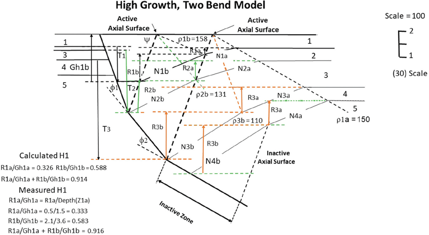
Figure 11-56 This multibend model may look more realistic than the previous models and tends to look more like some real structures. The model employs two active axial surfaces emanating from two bends in the fault. In order to solve Eq. (11-29), three inactive axial surfaces, R1a, R2a, and N1a, are used to form the triangles (see text for details). Horizon H5 has moved through the deepest active axial surface in the major fault, and thus the shape of the top of Horizon H4 is the same as Horizon H5. (Published by permission of R. Bischke.)
Domain 1.
The first domain group of solutions involves the structural relief of domain R1a. This involves the growth axial surface ρ 1a = 150 deg, N1a, and the active surface (ψ) to form the first triangle. The second problem also involves the growth axial surface related to ρ 1a dipping at 150 deg, the active axial surface, and N2a. The third set of solutions involves the triangle formed by ρ 1a and ρ 3b dipping at 110 deg and N3a. and not the angle (ψ) (Fig. 11-56). As the left-hand side of the triangle is not the angle (ψ) but ρ3b = 110 deg for this triangle, (ψ) is replaced by ρ3b = 110 deg when formulating Eq. (11-29). Also, for the measured values of Rna/Ghna, the Ghna values are measured at 1.5, 3.5, and 5.95 units.
Domain 2.
The second domain Rnb/Ghnb are solved next. The three triangles are formed by ρ 1b = 158 deg, N1b, and the shallowest active axial surface (ψ) at the first bend in the fault. Next, ρ 2b = 131, Nb2, and the active axial surface form a triangle. The last problem involves ρ b3 dipping at 110 deg, Nb3, and the active axial surface located at the second bend in the fault (Fig. 11-56). Horizon H4 is in the inactive zone of no deformation and has the same values as H3 (Fig. 11-56). In this case, the Ghnb values are larger than Ghna values in the first domain.
As there are two dip domains for each horizon, in order to determine the correct values of Rn/Ghn, the value of R1a/Gh1a is added to the value of R1b/Gh1b values. Figure 11-56 shows the measured and calculated values R1a/Gh1a and R1b/Gh1b along with the sum of the two values.
The Pregrowth Structure and Calculations section provides additional discussion on changing growth axial angles and how to model changing growth axial surfaces on real rollover structures. The large Gn variations in this modeled structure test the viability of the Rn/Ghn projection methods (Figs. 11-56 and 11-57). The Rn/Ghn value calculations using Eqs. (11-28) and (11-29) have an R-square of 0.9986 even though Gn = 82% (Fig. 10-57). This linearity at high Gn values is probably the result of a constant growth axial surface. In this case, the measured R-square is equal to 0.9999 and is a direct linear measurement, measured with a scale. Real structures (e.g., Figs. 11-61, 11-62b and c) also can have high R-squares, as do modeled structures. However, the growth model study, which includes other models not shown, suggests that the projection methods are often less reliable if the Gn % difference calculations exceed about 50% to 70%. The study of model structures predicts that the only structures that cannot be projected to greater depths are structures in which random horizon thicknesses (Gn) are present or in which the growth axial surface (ρn) changes significantly.
Figure 11-57 (a) The Rn/Ghn measured and calculated values versus depth(Z) graph for multibend model in Figure 11-56. This graph has a relatively high % difference = 82%, but nevertheless, the linear regression R-square results are about 1.0, in this case probably due to a linear growth axial surface. Horizon H5 has moved into the inactive zone, having passed through the deepest active axial surface. (Published by permission of R. Bischke.)
Thorsen (1963), and other work on extensional growth structures (Bischke et al. 2006), suggests that random structures are not common. An exception would be structures that rapidly increase or decrease in growth with increasing depth or contain large unconformities. However, many real structures, described in the following Real Structures section, have near-linear R-squares.
In summary, as many real rollovers have curved frontal limbs, the two-bend models look more realistic [Fig. 11-56 has two fault bends (ϕ) of 20 deg each]. Each bend requires a τn and ρn calculation or measurement. How to calculate this type of structure is also covered in the Pregrowth Structure and Calculations section, but the calculations are relatively simple when using a spreadsheet. Every change in dip requires an axial surface (ψ). Again, if the left-hand side of the triangle is not the angle (ψ), but the angle ρμ, then for this triangle, ρμ replaces (ψ) in Eq. (11-28); in this case, use Eq. (11-29). Notice that on Figure 11-56, the structure moved through the deepest active axial surface and entered the inactive zone.
Real Structures
Real structures can be observed in both seismic and well log data. Seismic data is described first. Published public domain 3D, depth-corrected seismic data are not common, probably for several reasons, including proprietary issues. First, vertically expanded data, such as time data, expand the vertical component of the time section, making correlations and sequence boundaries more obvious. Second, depth correction takes more time. In contrast, in compressional regimes, non-depth-corrected seismic data can lead to major interpretation problems (Chapter 10), although this distortion of geometry is less problematic in extensional regimes. Nevertheless, simply converting a depth-corrected seismic line with a local or regional velocity/depth function permits geoscientists to view the prospect on a scale that is closer to one to one and presents a less distorted view of the actual geometry. Chapter 9 discusses in detail the modern depth-correction process, mapping methods, and techniques involving several 3D shale basin data sets.
Seismic
Southern Louisiana Rollover.
Figure 11-58a is a measured Rn and throw(Tn) diagram from an older depth-corrected 2D line taken from Xiao and Suppe’s (1992) paper on the origin of rollover. This seismic line was one of the first balanced lines for extensional structures. Horizon H6 was not included in this calculation, as its base is a pregrowth horizon. Horizon 5, which is a multibend horizon, was divided into two-line segments with different dips and depths (Zn) (see Fig. 11-56 for an example). Four active axial surfaces, ψ = 67 deg, were constructed at the position where the base of divergence of horizons H2 to H5 intersect the fault surface. The throw(Tn) correlations of y to x is high, and thus the R-squares results are high at 0.973, indicating roughly linear slip with increasing depth (Fig. 11-58a).

Figure 11-58 (a) The throw (T) correlation has a high R-square and thus the slip on the fold is near constant. (b) The depth-corrected balanced structure from southern Louisiana is published in Xiao and Suppe (1992). On this rollover, the growth axial surface for the first three horizons have about a constant growth axial surface at the base with ρ1 = 139 deg, which then decreases its dips to a lower angle with ρ2 = 164 deg at the top of H4. Thus, the crest of structure widens at depth. Both the measured and calculated R-squares are near linear, even though the Gn % difference = 67%. (c) The anomalous horizon must lie on or near the near-linear formula at a depth of about 4.2 km. This calculated depth can then be mapped onto the crest of structure. (Published by permission of R. Bischke.)
The base of horizons H2 to H4 have a growth axial surface with ρ = 139 deg, although the base of Horizon H5 shifts to the right and the value for ρ2 = 164 deg. This makes the rollover slightly nonlinear. However, both the measured and calculated Rn/Ghn data have a high R-squared even though the horizon thickness Gn % difference = 67% (Fig. 11-58b). This high variance is caused by the large change in the growth axial surfaces (ρn) and the horizon thicknesses (Gn) that change with depth. The high R-squares result from a near-uniform growth axial surface (ρn) for the base of horizons H2 to H4. In Figure 11-58b, the calculated and measured linear regression values are 0.996 and 0.965 respectively. Remember that for the left-hand side of the shallow triangle on the base of Horizon H5, which bends from τ = 5 to τ = 12 deg,ψ must be replaced by ρa = 98 deg in Eq. (11-29). This rollover expands and the horizons diverge or thicken with depth (consult the Gn numbers in Fig. 11-58b).
Next, let us assume in the case of this near-linear structure that a sand or high TOC shale exists in a footwall well below the top of Horizon H4 at a depth of 3.18 km (see Xiao and Suppe 1992, their Fig. 20, at 3.18 km) but has not been penetrated in the hanging wall. As the measured data are near linear, and the base of horizons H2 to H5 were mapped in the hanging wall and footwall, it is possible to estimate the depth of this high TOC horizon in the hanging wall within some degree of accuracy. This accuracy can be estimated using the determined R-square values and then comparing these values to a perfect R-square value of 1.0.
First, the % difference of the footwall depths are calculated for Horizon H4 at 2.92 km and the horizon of interest by calculating the depth to the top of Horizon H4 and subtracting the depth to the horizon of interest. This value is then divided by the Horizon H4 thickness (as shown in Fig. 11-59), which equates to 0.704% for the footwall. Thus, in the hanging wall, the high TOC zone is located at about at a thickness of 70.4% below the top of Horizon H4. Based on near-linear growth, Figure 11-59 also shows the estimated depth to where the high TOC horizon is located in the hanging wall. This calculated depth near the fault is at about 4.2 km (Fig. 11-59).
Figure. 11-59 Profile showing how to calculate depth values for a horizon of interest located in the footwall and then calculate its approximate depth in the hanging wall. (Published by permission of R. Bischke.)
There is a check on this work that involves the linear regression y-x formula. As the measured data are near linear, the best depth estimate of 4.2 km for the TOC horizon is inserted into the growth formula. Next, the Rn/Ghn value times its depth should plot as a point along the measured near-linear trend (estimated depth on Fig. 11-58c). The y-x formula values were calculated before the insertion of the depth of the TOC horizon at 4.2 km in the hanging wall. The estimated value for Rn/Ghn = 0.1473 should lie along the measured data trend line (Fig. 11-58c).
Corsair Trend/Brazos Ridge Offshore Texas
Figure 11-60 is a tracing of a depth-corrected seismic line drawing of horizons construction by Xiao and Suppe (1992) with the help of a major oil company. A good discussion of the major producing Corsair trend, offshore Texas, is found in Vogler and Robison (1987). The 2D line is imaged in Figure 11-58a, b, and c.
Figure 11-60 A tracing of Figure 11-1 for a depth-corrected line drawing by Xiao and Suppe. The structure was fit to the line tracing. (Published by permission of R. Bischke.)
Figure 11-1a is from the large Corsair fault, which exhibits obvious bed dip divergence associated with large changes in the dip of the Corsair fault and large throws exceeding 10,000 ft (3 km) (Christiansen 1983). The beds dip toward the fault with maximum dip of 24 deg at a depth of 2.5 km. The depth-corrected line tracing was constrained by numerous deep wells that were drilled into the Big Hum, producing zone to depths exceeding 17,000 ft (5 km) (Vogler and Robison 1987). The line drawing generated by Xiao and Suppe is published in Tearpock and Bischke (2003) (Fig. 11-1). In Figure 11-60, the line drawing was slightly restored by removing crestal faults with small displacements (Fig. 11-12). The growth on this large rollover decreases with depth, as ρ1 dips at 135 deg at shallow depths, and ρ2 dips at 161 deg at deeper depths (the dashed lines on Fig. 11-60).
In Figure 11-61, measurements taken from this two-bend depth-corrected line is presented in the form of as Rn/Ghn graph. In spite of the changes in the growth axial surfaces and large thickness changes (the Gn % difference = 100%), the R-squares are near 1.0 (Fig. 11-60).
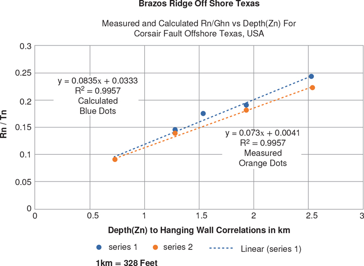
Figure 11-61 The measured and calculated Rn/Ghn values for a depth-corrected rollover from the Corsair fault, offshore Texas. This profile is a line tracing generated by Xiao and Suppe that was published in Tearpock and Bischke (2003) (Fig. 11-1). A restored model of Figure 11-1 is shown in Figure 11-60. Both the calculated and measured points on the figure were generated from a linear regression. These high R-square results from the linear regression occur in spite of large changes in horizon thicknesses with a Gn % difference = 100%. (Published by permission of R. Bischke.)
Haynesville Shale Play, Texas/Louisiana
The next example is a 3D depth-corrected line from the Haynesville shale play from Texas/Louisiana (Fig. 11-62a). This salt-related example images a fault that bottoms in a salt weld at about 15,500 ft (4.7 km). The first three horizons exhibit linear growth with the beds dipping from 4.5 to 7.5 deg. The measured and calculated Rn/Ghn values have R-squares at about 1.0, with horizon thicknesses of Gn % difference = 40% (Fig. 11-62b). The slope of the graph is positive, indicating increasing growth with depth (flat to dipping beds).
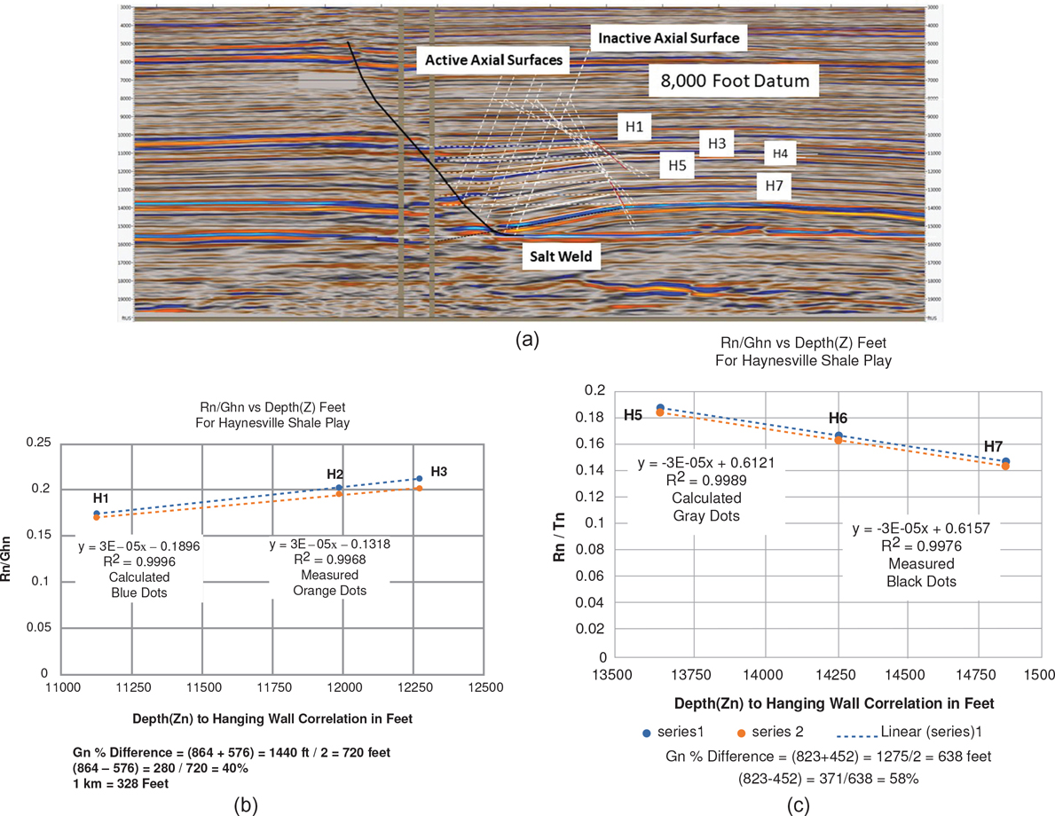
Figure 11-62 (a) This depth-corrected 3D line is from the Haynesville shale play trend in Texas/Louisiana. The large fault bottoms in a salt weld. Horizons from H1 to H3 diverge between 10,000 to 13,000 ft (3 to 4 km). (b) Measured and calculated Rn/Ghn values for horizons H1 to H3 between 10,000 ft on the crest of structure to 13,000 ft (3 to 4 km). Calculated and measured Rn/Ghn values are near linear. (c) R-square values = 0.9988 for a decreasing growth of horizons H5 to H7 directly above the salt weld. (Published by permission of R. Bischke.)
The three horizons above the salt weld also exhibit linear growth, but in this case with a negative slope indicative of decreasing growth with increasing depth (Fig. 11-62c). Above the salt weld, the bed dips range from 9.5 to 10.5 deg. The measured R-square values are also at about 1.0, with a Gn % difference = 58%. Horizon H4 is a probable unconformity, does not fit the two linear trends, and exhibits decreasing growth.
Starting at the base of Figure 11-62c and working toward the surface, an interpretation of the tectono-stratigraphy is as follows. At first, the sediments loaded the salt as the sediments thickened upward to Horizon H5 (increasing growth, growth is in dimensionless time; see Chapter 13). The thicken upward sequence was linear and ended at Horizon H5. There was a change in growth resulting in the unconformity at Horizon H4. Then the growth decreased linearly (Fig. 11-62b) until the sedimentary loading expelled all of the salt, creating the weld. This event happens at the flat horizon above Horizon H1 (see Fig. 11-62a). This sequence style was first described by Thorsen (1963) using the expansion index (Ei) for the Norco, Bonnet Carre faults and in particular on the LaPlace fault (Fig. 13-3).
Well Log Data
The last example is a near-linear example of growth using well log data. This example uses missing section data from the Rabbit Island Field, Louisiana (Fig. 11-63a, interpreted by Dan Tearpock). The wells cut a downward dying fault and its fault surface map along with a seismic line is published in Tearpock and Bischke (2003) (see Fig. 13-27). At shallow depths, the missing section values increase, and then decrease below a depth of about 5600 ft (1 ft = 0.3048 m). The seismic line exhibits coherent data at about 11,000 ft, and a well at this level contains a complete stratigraphic section with no faulting to trap hydrocarbons (Tearpock and Bischke 2003). The missing section data are not precisely linear (mostly the result of the deepest correlation point) but are readily fit to a second-order polynomial with an X-square coefficient of only 7xE-06. However, if the missing section data are analyzed from the 5700-to 9700-ft level, the data are nearly linear (Fig. 11-63b). This portion of the Rabbit fault slipped at a near constant distance.

Figure 11-63 (a) This figure uses missing section well log data interpreted by Dan Tearpock. This example is constrained by a fault surface map and a seismic dip line that crosses the fault (see Fig. 13-27). The wells cut a downward dying fault from the Rabbit Island Field, Louisiana, that is published in Tearpock and Bischke (2003). Below 5500 ft, the missing section decreases from 490 ft to 70 ft (Fig. 13-27). The missing section data are best fit to a second-degree polynomial that contains a small coefficient of 7E-06. Thus, if the deepest data point is eliminated, the data are almost linear. (Published by permission of R. Bischke.)
Unconformity in Shale Basin
Figure 11-64a shows a shale basin 3D seismic line with a large unconformity between the H3 and H4 horizons, indicating that not all growth is near linear and that unconformities can cause nonlinear growth. Figure 11-64b is a plot of the growth discontinuity (Bischke 1994b) in which Horizon H3 is clearly offset from the averaged R-square general trend using all four data points.
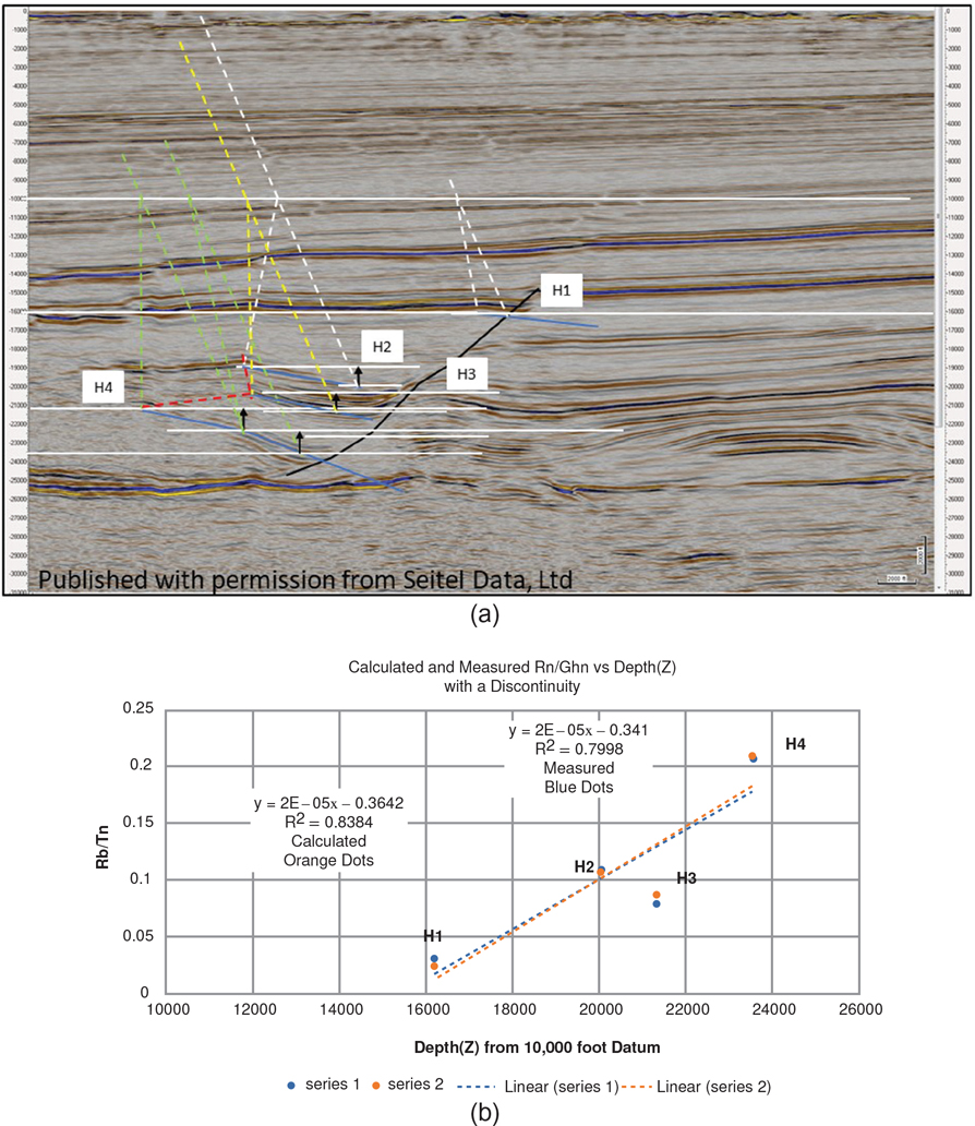
Figure 11-64 This figure is a shale basin example that contains an unconformity and therefore nonlinear growth. The existing discontinuity in growth is clearly present on the growth diagram, as Horizon H3 is offset from the general trend (Fig. 11-64b). (Published by permission of R. Bischke.)
Most of the generic and real examples shown exhibited near-linear coefficient correlations of the crestal data. The example in Figure 11-64a is more complex and exhibits a changing growth axial surface (red lines), and thus this example has high R-squares (Fig. 11-64b). A large unconformity offsets the structure along the near horizontal portion of the dashed red line, as the unconformity shifts the crest of structure to the left.
Conclusions
This study started by discussing linear growth in general and then concentrated on which factors affect linear growth on generic models, finally applying these results to several real data. Many real examples were subject to the linearity tests. Growth becomes less linear if the % difference calculations exceed about 50% to 70%. Data become less linear if the growth is large and variable, alternating between increasing then decreasing growth, or if the growth axial surface (ρ) changes dip. Many seismic sections exhibit nonlinear growth, particularly if the section contains a large unconformity (Fig. 11-64).
Public domain, depth-corrected seismic data are not common in the literature, and thus firm conclusions regarding near-linear growth on numerous real structures is unavailable. The section Real Structures and examples presented in Chapter 13 on growth structures show that near-linear growth exists in well log data and on some older, depth-corrected 2D seismic data. Our study of 3D seismic and depth-corrected seismic show that episodes of near-linear data, obtained from Chapter 9, exist in shale play basins.
Linear growth may have applicability for the following reasons. First assume that linear growth is present in both the footwall and the hanging wall. If an interesting horizon, for example, either a hard shale or a high TOC section, is present in the footwall but has not been penetrated in the hanging wall, then projecting the footwall interval to depth in the hanging wall is possible. Next, run a linear regression analysis of the depths in the known footwall intervals. This analysis results in a y-x equation. The depth of the interesting interval in the hanging wall will lie on a Ghn/depth (Z) graph of the linear equation.