Chapter 7. Fault Maps
Introduction
Faulted structures play a very significant role in the trapping of hydrocarbons. Therefore, it is imperative that anyone involved in the exploration for, or exploitation of, hydrocarbons should have a significant understanding of faults within the area of study, including their origin and relationship to the formation of structures. Detailed interpretation and mapping of major faults is critical in the process of hydrocarbon exploration and development. This chapter presents the correct subsurface interpretation and mapping techniques required to prepare fault surface maps. Chapter 8 presents the techniques for integrating faults into structural interpretations and maps. Faults themselves are vital to structural development and to hydrocarbon migration and entrapment. A reasonable structural interpretation, in faulted areas, begins with an accurate fault interpretation resulting from the construction of fault surface maps and the proper integration of these fault maps into the structural interpretation. We refer to constructed fault maps as fault surface maps rather than the more commonly used term “fault plane maps,” since most fault surfaces are not true planes.
The data required to construct a fault surface map are obtained from the correlation of well logs, interpretation of seismic sections, and at times from outcrops. In Chapter 4, we present the methods and procedures for recognizing a fault in a well log and determining its missing or repeated section. In this chapter, we discuss the importance of mapping faults and present the methods for constructing fault surface maps with fault data acquired from electric well logs and seismic sections.
The preparation of accurate fault surface interpretations and maps requires a strong geological background, 3D thinking, and a good understanding of the structural style of the area being worked. When we make reference to the understanding of structural style, we are referring to that specific assemblage of geological structures common to a particular petroleum province (Fig. 7-1). In order to prepare geologically reasonable maps, one must be familiar with the tectonic setting being worked, the fault and structural patterns expected, their origins, and, at times, the process of development. Many of the basic concepts, methods, and techniques for interpreting and mapping faults are universally valid. However, their recognition, interpretation, map construction, and application very much depend on the geoscientist’s background and understanding of the kinds of geological structures being worked (see Chapters 10, 11, and 12).
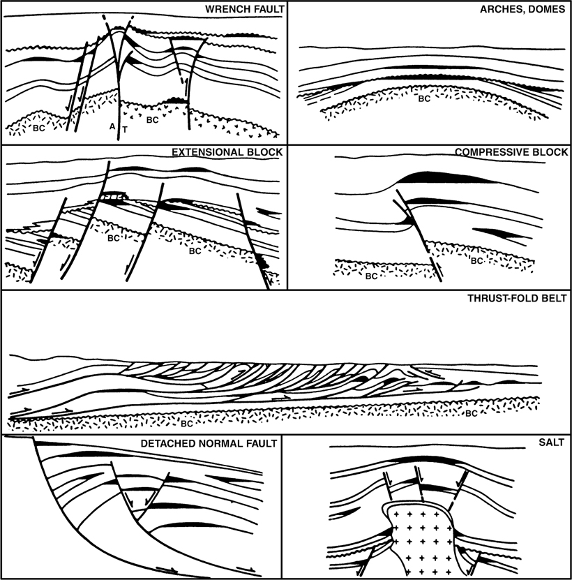
Figure 7-1 Schematic diagrams of hydrocarbon traps associated with various structural styles. BC, basement complex; T, displacement toward viewer; A, away from viewer. (From Harding and Lowell 1979; AAPG©1979, reprinted by permission of the AAPG whose permission is required for further use.) (Salt-related closures modified from Salt Domes by Michel T. Halbouty. Copyright 1979 by Gulf Publishing Company, Houston TX. Used with permission. All rights reserved.)
Detailed discussion of structural geology or structural styles is beyond the scope of this text, although many aspects of this subject are presented in several chapters, including Chapters 9, 10, 11, and 12. We consider this book to be an advanced level text with the focus on structural and mapping techniques, and we make the assumption that you have a general understanding of the fundamental principles of classic geological study, including structural geology as outlined in such texts as Billings (1972), Harding and Lowell (1979), and Suppe (1985).
Faulted structures can be simple or complex. To provide the best structural interpretation with the available data, the integrity of the structure must be shown to be sound and geologically reasonable. To provide the soundest and most accurate geological interpretation in faulted areas, the interpretation, mapping, and validation of the faults is the first step. The construction of fault surface maps as a fundamental part of any geological study is absolutely necessary. The integration of fault surface maps with structure maps is also essential to support the structural interpretation, to prepare accurate maps, to identify prospects, to design wells to be drilled, and to determine the volume of potential hydrocarbons. The integration of fault and structure maps is discussed in detail in Chapter 8.
Too often, geological interpretations and the accompanying maps and cross sections are prepared without giving much consideration to the 3D geometric validity of the interpretation. Testing the validity of geological interpretations is discussed in some detail in Chapter 10 under structural balancing, but it needs to be stated here that the proper construction of fault surface maps and their correct structural integration can go a long way toward providing 3D validity or consistency to any interpretation.
It is not sufficient to rely solely on what the well logs are indicating or what is seen on the seismic sections. Cross sections and seismic sections can in themselves misrepresent true subsurface relationships by the simple nature of their orientation as well as by other factors. A good understanding of 3D geometry is essential to any attempt at reconstructing a subsurface picture.
No hydrocarbons have ever been trapped by a fault trace. The trap is along the fault surface itself. Therefore, the mapping of the surfaces of all-important faults is an integral part of any subsurface interpretation, particularly in areas involving multiple faults, where extremely complicated structural relationships can exist. Attempting to reconstruct a complicated structure by using isolated fault data from electric well logs or seismic sections without the benefit of reasonable fault surface maps and their integration with various structural horizons can provide erroneous geological interpretations. Shortcuts are often taken in our preparation of subsurface maps. Such shortcuts include failure to construct fault surface maps, the preparation of a structure map of only one horizon, or the use of a limited number of seismic sections to generate an interpretation. In this chapter and in Chapter 8, we show how such shortcuts can often lead to structural interpretations that are misleading, unreasonable, and therefore costly to any exploration or development program.
The basic concepts and techniques discussed in this chapter apply to the use of data obtained from both vertical and deviated wells in addition to data from seismic sections. The discussions, illustrations, and practice problems deal principally with extensional and compressional faulting that reflect mainly dip-slip movement, but the methods are broadly applicable to all styles of faulting.
Fault Terminology
“Probably no portion of geological literature has a more confused terminology than that dealing with faults.” This is a profound statement that is as applicable today as it was when made by H. W. Straley in 1932. A literature search on the subject of fault nomenclature, or terminology, shows that as far back as the turn of the century, there was great inconsistency in the use of fault component terminology.
In 1908 the Council of the Geological Society of America appointed the Committee on the Nomenclature of Faults. This committee was charged with establishing proper fault nomenclature. Since that time, there have been numerous papers on the subject of fault components and their related terminology, usage, and nomenclature. However, despite these numerous publications, many geoscientists and engineers are still confused when it comes to the definitions and usage of various fault component terms.
The correct understanding and usage of fault terminology with respect to certain fault components is essential to the preparation of correct subsurface fault and structural interpretations and maps. Therefore, in this section we discuss the fault components that are important to subsurface mapping in the petroleum industry. Many others are not discussed, not because they are less important but because they do not apply to the interpretation and mapping techniques that are presented in this text. Figure 7-2 graphically defines several of the fault components of interest to us.

Figure 7-2 Block diagram of Bed X displaced by a normal fault, illustrating four different fault components. The front panel is perpendicular to the strike of Fault F-1. (Modified from Tearpock and Harris 1987. Published by permission of Tenneco Oil Company.)
In the literature, the definitions and uses of the terms vertical separation, throw, and heave are inconsistent and confusing. The correct usage of fault component terms by all geoscientists and engineers may never be achieved. However, in order to correctly conduct interpretations and construct subsurface maps, we must use the fault component terms vertical separation, throw, and heave in a consistent manner. We choose to use the terms as follows.
Vertical separation (AE) is the vertical component of bed displacement. It is measured as the vertical distance between a horizon (such as the top of a stratigraphic unit) projected from one fault block across a fault to a point where the projection is vertically over or under the same horizon in the opposite fault block. It is that separation seen in vertical wellbores, vertical shafts, and vertical cross sections (Dennis 1972).
Throw (AC) is the difference in vertical depth between the fault intersection with a horizon in one fault block and the fault intersection with the same horizon in the opposing fault block, determined in a direction perpendicular to the strike of the fault surface.
Heave (BC) is the horizontal distance between the fault intersection with a horizon in one fault block and the fault intersection with the same horizon in the opposing fault block, determined in a direction perpendicular to the strike of the fault surface.
Missing section is the vertical thickness of the stratigraphic section faulted out of a wellbore as a direct result of a normal fault cutting through the section. Missing section is sometimes referred to as fault cut. Repeated section is the vertical thickness of the stratigraphic section repeated in a wellbore as the direct result of a reverse fault cutting through the section. The missing or repeated section is determined by correlation of an electric log from one well with other electric logs from nearby wells, as presented in Chapter 4. Technically, missing or repeated section is equal in value to vertical separation. Vertical separation for a fault can also be determined from seismic data, as shown later in this chapter.
We cannot overemphasize the importance for all geoscientists and engineers to understand that the missing or repeated section recognized in well logs is NOT throw, nor is it equal to throw, but rather that it is equal to the fault component vertical separation. A misunderstanding of the technical point can create, and has caused, significant interpretation and mapping errors resulting in millions of lost dollars from dry holes, failed recompletions, workovers, and more. Of special interest is the integration of well log with seismic data. Major interpretation errors occur regarding fault displacement when seismic data are misinterpreted by using throw, or apparent throw, determined from seismic sections as if it were equivalent to the missing section from nearby wells.
Notice in Figure 7-2 that the value for the throw of the fault is not equal to the value for the vertical separation. The fact that they are different components of a fault is of significance when fault data obtained from well logs are used for integrating faults into a structural interpretation (Tearpock and Bischke 1990). The terms throw and vertical separation are commonly misunderstood and, more importantly, often misused in the preparation of subsurface interpretations and the accompanying fault and structure maps.
Because the understanding of these terms is so important to correct interpretation and construction of subsurface fault and structure maps, we attempt to clarify the issue without causing more confusion than currently exists. We discuss the terms in a general way and review them with respect to subsurface mapping techniques. For a complete review of the subject of fault nomenclature, refer to the references at the end of the book.
Definition of Fault Displacement
We apply a definition to the word displacement similar to that given by Reid et al. (1913). It is here applied to the relative movement of the two sides of a fault, measured in any specified direction, or to the change in position of a marker or horizon caused by fault movement. There are two ways to estimate displacement resulting from a fault. The first is the actual relative displacement of the two sides of a fault, and the other is the apparent relative displacement.
Slip is the actual relative displacement of a fault (Hill 1959). It is defined as the measurement of the distance of the actual relative motion between two formerly adjacent points on opposite sides of a fault, measured on the fault surface. Separation is the apparent relative displacement of a fault (Hill 1959). It is defined as the distance, measured in any specified direction, between two parts of a displaced surface on opposite sides of a fault. Separation is apparent movement on a fault with respect to a reference horizon cut by the fault (Dennison 1968). Separations are measurable, whereas slip is usually calculated. Numerous authors (including Reid et al. 1913; Hill 1947; Crowell 1959; Dennis 1972; Tearpock and Harris 1987; Tearpock and Bischke 1990; and others) have emphasized the importance of distinguishing between fault components related to slip and those components related to separation.
We emphasize that components of the actual slip cannot routinely be measured in the subsurface due to a lack of conventional sources of data from which the measurements can be made. Therefore, slip components are not routinely mappable. Some separation components, on the other hand, are measurable fault components with conventional subsurface data and therefore are mappable. They can be measured in a vertical shaft, an electric log from a wellbore, or on a seismic section, regardless of orientation with respect to fault strike. Of these various separation components, vertical separation is the most important parameter for constructing subsurface fault and structure maps (Tearpock and Harris 1987).
Throw and heave cannot be measured by correlation of well logs, as we will demonstrate. Using a seismic interpretation, measurements of throw and heave can be made only if the interpreted seismic profile is oriented perpendicular to the strike of the fault surface. The terms throw and heave have limited practical application in subsurface petroleum interpretation and mapping. In addition, they cause confusion and significant interpretation and mapping errors. We discuss their application and relationship to other fault components later in this chapter and again in Chapters 8.
We cannot leave this subject with the idea that fault slip is not important. Fault slip and related components are important, particularly in mining operations. Slip generally can be determined in mines where the actual fault surface is visible. In fact, the usage of the terms throw and heave originally came from the coal fields of Great Britain where the strata are nearly horizontal or the faults are strike faults (Reid et al. 1913). As mentioned earlier, these terms have found their way into the petroleum industry and are probably here to stay. However, they have limited practical application in subsurface petroleum interpretation and mapping.
Mathematical Relationship of Throw to Vertical Separation
Throw can be measured in cross sections drawn perpendicular to fault surface strike (or parallel to maximum dip), such as Figure 7-3.
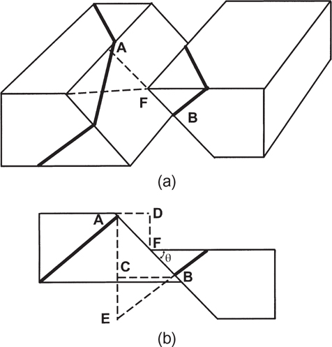
Figure 7-3 (a) Block diagram showing surface displaced by normal fault. (b) Vertical cross section perpendicular to strike of fault; in same plane as front of hanging wall block of block diagram. DF is vertical slip; AD is horizontal dip slip; AC is the throw; BC is the heave; AE is the vertical separation. DF, AC, and AE are all used by some geologists as throw. (Modified from Billings 1972. Published by permission of Pearson Education, Inc.)
where
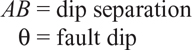
Thus, as the fault changes dip, the value of throw must also change. We emphasize at this point that throw (which is related to fault dip and displacement) cannot be directly measured from electric well logs. We do, however, present methods that enable you to calculate the amount of throw, if desired, knowing the vertical separation and other properties, such as fault and bed dips. However, throw does not normally enter into proper subsurface mapping techniques (Tearpock and Bischke 1990).
The vertical separation (AE) in Figures 7-2 and 7-3 is defined as the distance that a bed has been vertically displaced during faulting (Hill 1947). This distance is of primary importance to us because the vertical separation is recognized and determined from correlated electric well logs, as described in Chapter 4. To illustrate this point, consider the following example. Assume that a structure exists that contains beds that dip uniformly to the west (Fig 7-4). The SP from two wells drilled into these beds is shown on the figure. The dashed line in Figure 7-4 represents a future normal fault. The beds will be displaced in such a manner that the hanging wall portion of Well No. 1 is placed in juxtaposition with the footwall portion of Well No. 2, as shown in Figure 7-5.
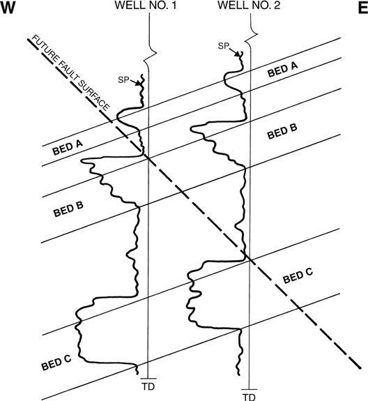
Figure 7-4 Hypothetical example. Unfaulted structure with beds dipping uniformly to the west. Dashed line shows location of future normal fault perpendicular to plane of cross section. (Published by permission of D. Tearpock and R. Bischke.)
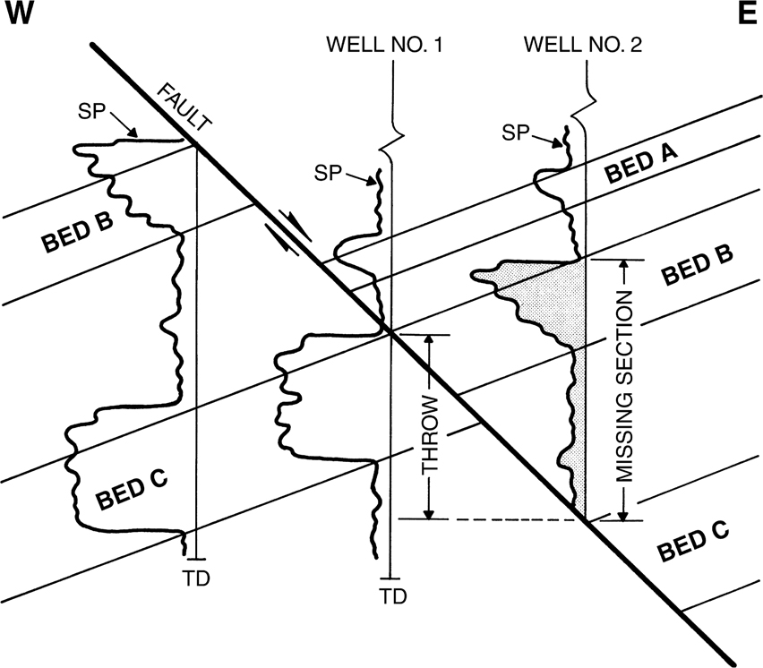
Figure 7-5 Beds are displaced such that the upper portion of Well No. 1 in the hanging wall fault block is juxtaposed with the lower portion of Well No. 2 in the footwall block. Missing section in Well No. 1 by correlation with Well No. 2 is highlighted on the SP curve for Well No. 2. The missing section is equal to vertical separation and not to throw. (Published by permission of D. Tearpock and R. Bischke.)
The geometric configuration produces the following observations in Figure 7-5. As the hanging wall block is displaced, the top of Bed B in the hanging wall is brought into contact with the top of Bed C in the footwall. Therefore, the missing section in Well No. 1 of the hanging wall includes the stratigraphic section from the top of Bed B to the top of Bed C. Inspection of the electric well logs now reveals that the missing section as the result of the fault in Well No. 1 (in the hanging wall) is represented by the coarsening upward sand sequence and the lower shale section present in the hanging wall portion of Well No. 2 (shaded section in Fig. 7-5).
This example clearly demonstrates that the throw of the fault is not equal to the missing section in the faulted well. However, the missing section is equal to the vertical separation as defined in Figures 7-2 and 7-3. We therefore have shown that electric well logs record vertical separation and not throw and that throw does not directly enter into subsurface mapping techniques (Tearpock and Harris 1987; Tearpock and Bischke 1990). Vertical separation (as well as throw) varies laterally and with depth on a fault. Expect these variations and be prepared to recognize them in your interpretation of well and seismic data, and honor the variations in your maps of faulted structures.
Quantitative Relationship
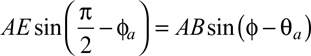
Vertical separation can be related to throw (Tearpock and Bischke 1990) through two equations, which change with bed dip (Eqs. 7-1a and b), and these equations are derived from Figures 7-6 and 7-2. Performing some trigonometry and using the law of sines, the following relationship is developed:
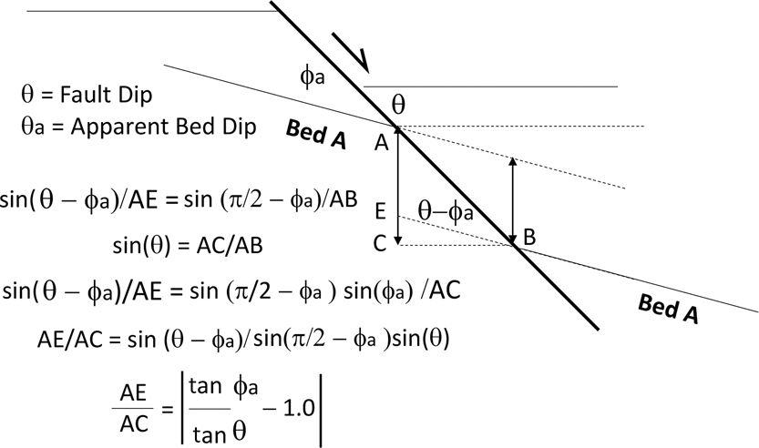
Figure 7-6 Using trigonometry and the law of sines, the relationship of vertical separation to throw is shown graphically in this figure and mathematically in Eq. (7-1a). (Published by permission of D. Tearpock and R. Bischke.)
Substituting
yields
Utilizing trigonometric identities yields

where

If derived from Figure 7-2, and there is missing section between the hanging wall and the footwall, then
Equations (7-1a) and (7-1b) have application in regard to the evaluation of subsurface structure maps (Tearpock and Bischke 1990). This 2D equation gives us the ability to check completed structure maps for accuracy of construction when the missing or repeated section is used to prepare an integrated subsurface structure map (see the section Contouring Faulted Surfaces in Chapter 8 for definition of integrated structure map). In Chapters 7 and 8, we discuss the application of Eq. (7-1a) to test the validity of structure maps constructed using well log or seismic data, and we present a method for analyzing the magnitude of error if mapped incorrectly.
Using data from the first edition of Applied Subsurface Geological Mapping (Tearpock and Bischke 1991), J. R. Sonnad generated a 3D equation for determining throw. The geometric relationships here are similar to those presented in Chapter 4 regarding the Setchell equation. Therefore, the data are used to establish the 3D equation for calculation of throw when the required fault and structural data are available.
where
ϕ = true bed dip
α = azimuth between bed dip direction and fault dip direction
θ = true fault dip
Fault Data Determined From Well Logs
As a standard practice in reviewing subsurface structural interpretations and accompanying maps with faults, two questions should be asked: (1) What fault data were used to estimate amounts of missing or repeated section for the fault or faults in the preparation of the structure maps? (2) What technique was used to contour across the fault(s)? If the interpreter responds that throw was mapped across the faults and the source of the fault throw data was subsurface well logs or seismic sections, a review of the maps can easily be made to determine whether the use of the word throw is simply a verbal substitution for vertical separation or whether the interpreter actually used the vertical separation data incorrectly as if the data were throw. If fault data from electric logs were used as throw for a fault in the construction of an integrated subsurface interpretation, the structure map prepared will probably be incorrect and require revision. The use of well log fault data as throw in mapping across faults on structure maps is an incorrect technique. Herein lies one of the most basic problems with the construction of many subsurface structure maps—a misunderstanding of what fault data are actually obtained from electric well logs for use in subsurface structure mapping.
Determination of fault data begins with well log and seismic correlations. Although there have been numerous publications on fault component terminology covering the subject of throw and vertical separation, we were unable to find one figure that diagrammatically illustrates the geometric relationship of missing or repeated section, as seen on an electric log from a vertical wellbore, with respect to the fault components throw and vertical separation. Figure 7-3, from Billings (1972), illustrates a vertical cross section perpendicular to the strike of a fault surface showing such fault components as throw, heave, and vertical separation. Notice that the figure shows at least three separate fault components defined by various geoscientists as throw, demonstrating the confusion that surrounds the use of these fault component terms. Although this figure correctly illustrates the difference between throw and vertical separation, it does not relate this geometry to what is seen in a well log.
Since fault data are in part derived from well log correlation, it is very important to understand that the true vertical thickness of missing or repeated section, determined in a well by correlation of electric logs, is actually a measurement of the fault component vertical separation. The cross section in Figure 7-7 diagrammatically shows the geometric relationship between the missing section in a wellbore and the vertical separation of the fault. The east-west structural cross section, which is perpendicular to the strike of the fault surface, shows two beds (A and B) that have been displaced by the normal Fault F-1. This normal fault cuts Well No. 1 at −5230 ft and is dipping at an angle of 45 deg to the east. The beds are dipping at 30 deg to the west. By correlation with Well No. 2, the missing section in Well No. 1 is determined to be 100 ft and the fault is shown to have entirely faulted out Bed A in Well No. 1. As shown in the cross section, the throw of Fault F-1 is represented by the vertical line AC, which is equal to 63 ft. The vertical separation, represented by the vertical line AE, is equal to 100 ft. Thus, by the correlation of Well No. 1 with Well No. 2 in Figure 7-7, we have diagrammatically shown that the missing section obtained for the fault in Well No. 1 is not throw nor equal to throw but rather is a measurement of the fault component vertical separation. With this particular set of conditions, the throw of the fault is only 63 percent of the vertical separation. As shown in Figure 7-7, there can be a significant difference between the throw and vertical separation of a fault. If mapped incorrectly, this difference can result in significant error in an integrated structural interpretation and therefore the generated structure maps.
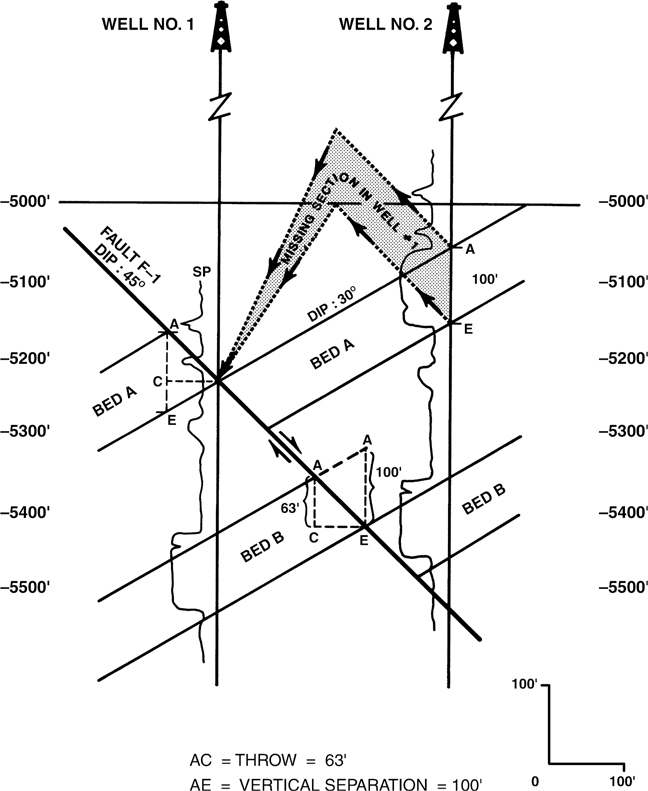
Figure 7-7 Diagrammatic cross section illustrates the geometric relationship between the missing section in a wellbore and the vertical separation of a normal fault. The 63-ft value of throw was calculated mathematically using Eq. (7-1). (Published by permission of D. Tearpock.)
For the most part, an understanding of fault terms and their application to subsurface mapping comes from academic studies and company-sponsored training programs. Textbook discussions on faults commonly use very simplistic examples showing faults cutting horizontal beds. These examples using horizontal beds lead to the misconception that throw and vertical separation are the same fault component or have the same value. Throw and vertical separation, however, have the same value in only three specific circumstances: (1) where the strata being faulted are horizontal, (2) where the fault is vertical, or (3) in a cross section perpendicular to the strike of the fault surface, where the fault strike is at a right angle to the strike of the strata. In the latter situation, the strata will have an apparent dip of zero deg. Figure 7-8a shows the situation involving horizontal beds where the values for throw and vertical separation are the same. The use of models where faults cut dipping beds (Fig. 7-8b and c) should eliminate the misconception that missing section is always throw, an idea that leads to the preparation of incorrect maps.
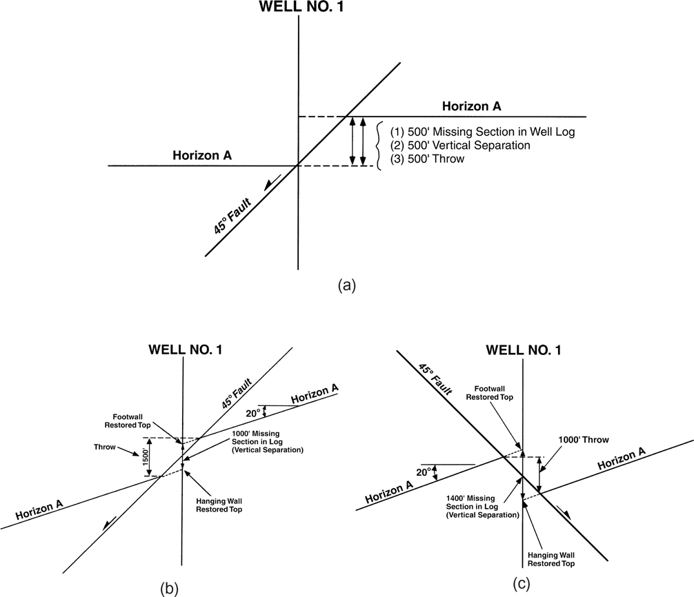
Figure 7-8 (a) The values for throw and vertical separation are the same where the displaced beds are horizontal. (b) Where both the strata and the fault dip in the same general direction, throw is greater than vertical separation. (c) Where the strata and the fault dip in generally opposite directions, throw is less than vertical separation. (Published by permission of D. Tearpock.)
The first set of conditions from our list of situations, where vertical separation equals throw, is discussed in greater detail here because it is the most common situation presented in textbooks and the one that has resulted in more misunderstanding of the fault component terminology than any other. Because of exposure only to simplistic examples using horizontal beds, many geoscientists and engineers have failed to recognize that the values for these two different fault components vary from each other depending on the structural attitude of the formation. This major misunderstanding can result in numerous mapping errors in a structural interpretation.
Figures 7-8b and c illustrate the discrepancy in values of vertical separation and throw where bed dip is considered. They further show the relationship where the horizons are dipping in the same general direction as the fault and where the horizons are dipping in the opposite direction to the fault. For example, as shown in Figure 7-8b, the missing section in Well No. 1 is 1000 ft, although the throw of the fault is 1500 ft. In Figure 7-8c, the missing section in Well No. 1 is 1400 ft, whereas the throw is only 1000 ft. We point out again that with the well logs, only vertical separation (missing section) data can be determined. Throw cannot be determined from well log correlation, but it is not important to know in most cases.
Vertical separation is directly measurable from correlation of well logs and is equivalent to the missing section or repeated section caused by a fault, which is valid regardless of the apparent attitude of any horizon considered. Throw and heave are dependent fault variables that change with variations in the apparent attitude of the fault and horizon. For most petroleum-related interpretation and mapping, the estimates for throw and heave have mainly academic value. They can be measured only in a cross section or seismic section that is oriented perpendicular to the strike of the fault surface, or on a structure map after the map has been completed using fault data correctly as vertical separation to construct a technically and structurally reasonable map. By using Eq. (7-2), however, the measured throw across a fault on a completed structure map can be used to check the accuracy of the map. This is discussed in detail in Chapter 8.
Fault Surface Map Construction
A fault surface map is a type of contour map. It differs from a structure contour map in that the contours are on the surface of a fault rather than on some stratigraphic marker or horizon. The contouring of a faulted horizon presents numerous complex problems, in the contouring of both key horizons and fault surfaces. Although the contouring of key horizons may be the main objective in a mapping project, the contouring of the fault or faults provides essential information about the geology being studied. We present more details on this subject in Chapter 9, which includes 3D diagrams and presentations.
In an area where a fault serves as the boundary limit of a hydrocarbon reservoir, the trap is along the fault surface itself. Construction of the geological picture involves the integration of all fault surface maps with several key structural horizons. Therefore, construction of an accurate fault surface map for each important fault, using all available data, is usually the first step in generating a structural interpretation where faults are present.
Earlier in this chapter, we mentioned that the preparation of accurate fault surface maps requires 3D thinking and a good understanding of the regional tectonics being studied. This is so because each tectonic setting has its own characteristic patterns of faulting. For example, most of the faults in areas like offshore Nigeria or the northern Gulf of Mexico Basin are normal faults typically downthrown to the basin and, although they may strike in any direction, the preferred strike direction is roughly parallel to the present or historical coastline. Regional knowledge is very important in developing a geological interpretation, comparing alternative geological solutions, and generating final subsurface maps that are geologically reasonable.
Note that we use the term fault surface map, or just fault map, instead of the more common usage of fault plane map. Fault surfaces tend to differ from true mathematical planes. They may increase or decrease in dip with depth, as well as change strike direction reflecting a sinuous or angular appearance, which may trend in a specific direction or represent an arcuate shape. In profile they may be listric, antilistric, or kinked. Some fault surfaces are deformed. Fault surfaces are therefore rarely perfect planes. However, on a very localized or field scale, some faults may appear planar and can be mapped as such. Some of the basic fault examples in this textbook represent idealized data used to present and teach a specific technique. In these cases, the fault examples are often simplified as true planes.
The construction of fault surface maps has numerous benefits in the interpretation and understanding of the development of faulted structures. Fault surface maps
aid in solving 3D structural problems;
define the location of a fault in space in both the horizontal and vertical dimensions;
help delineate complex fault patterns;
can be integrated with structure maps to delineate accurately the
upthrown and downthrown fault traces
fault gap or overlap
hydrocarbon reservoir limits;
are required to evaluate potential cross-fault drainage;
are required to construct fault surface sections (Allan diagrams);
can be used at times as an indication of the changing stratigraphy (sand/shale) in the footwall by means of a change in dip of the fault (see the section Inverting Fault Dips to Determine Sand/Shale Ratios or Percent Sand in Chapter 11);
eliminate the distortion of a fault as seen on a cross section with zigzag well spacing;
can be used to estimate the dip and strike of a fault at any location along the fault;
aid in the designing of well plans, particularly for directionally drilled wells; and
help identify prospects that otherwise might be overlooked.
In the subsurface, faults can be recognized in one of three ways: (1) through the correlation and interpretation of electric logs, (2) by the interpretation of seismic sections, and (3) by inference. In this section, we discuss the use of electric logs to obtain fault data required to construct a fault surface map. The fault information begins with fault data points in electric logs. These data points, which represent the intersection of a drilled well with a fault surface, establish the actual presence of faulting (refer to Chapter 4). For normal faults, the fault is usually represented by a loss of stratigraphic section, whereas a repeat of section is associated with reverse faults, as shown in Figure 7-9. There are exceptions to this generalization, however, such as the special case of steeply dipping beds cut by a normal fault, resulting in a repeated section, as shown in Figure 7-9c.
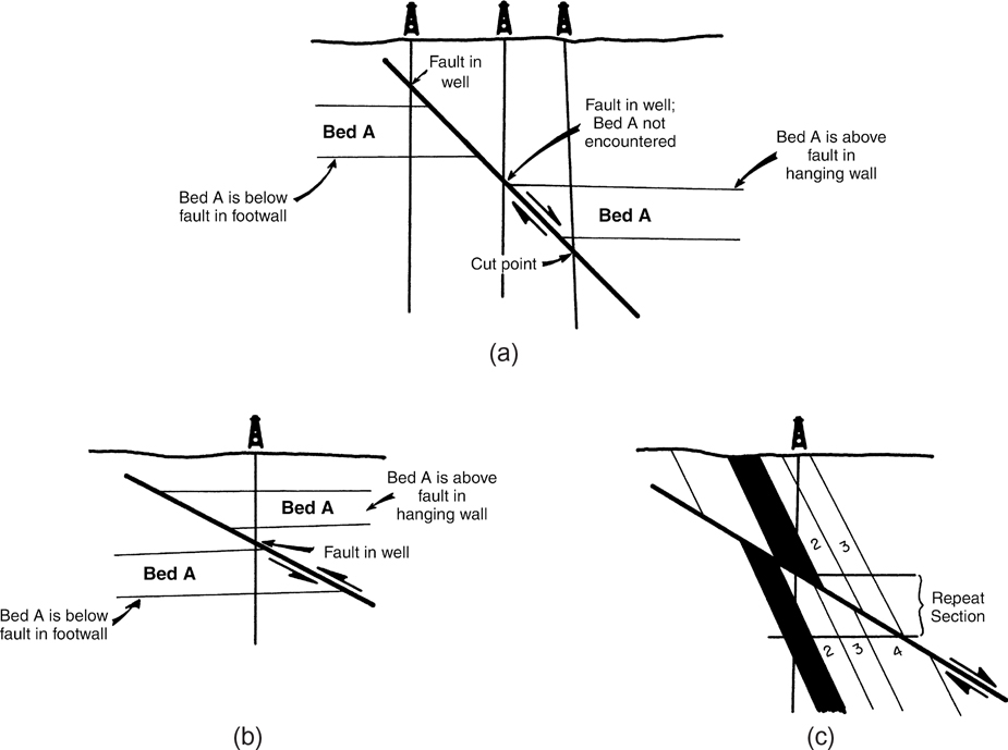
Figure 7-9 (a) Normal fault resulting in a missing section. (b) Reverse fault resulting in a repeated section. (c) Normal fault resulting in a repeated section. In example (c), the beds are dipping at a steeper angle than the fault. (Modified from Bishop 1960. Published by permission of author.)
For a normal fault, any key horizon encountered in a well above the fault is typically in the hanging wall (downthrown) fault block, and any marker encountered below the fault is in the footwall (upthrown) fault block (Fig. 7-9a and c). The only exception is in a deviated well crossing a fault backwards (Fig. 4-36), or on the flanks of salt domes. For a reverse fault, any horizon encountered in a well above the fault is in the hanging wall (upthrown) fault block; a marker encountered below the fault is in the footwall (downthrown) block (Fig. 7-9b). This relationship between the fault pick and any particular horizon thus indicates whether a well is in the footwall or hanging wall fault block for any particular horizon being mapped.
For each fault point in a well, two values are required for use in the interpretation and construction of a fault map: (1) an estimate of the amount of missing or repeated section for the fault, which we define as the vertical separation, and (2) an estimate of the subsea depth of the fault in the well. In Figure 7-10, the recognized fault data in the log of Well No. 2 are clearly marked to indicate the amount of missing section as a result of the fault (150 ft), the depth of the fault (a measured depth of 7280 ft), and the well(s) used in the correlation (Well No. 1). If you are still not sure how to identify faults in electric well logs, refer again to Chapter 4 on electric log correlation.
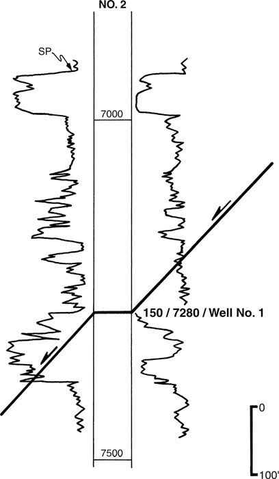
Figure 7-10 Fault information is documented on the electric log. It indicates the missing section, depth of the fault, and the well used for correlation.
Fault data from at least three wells, not in a straight line, are required to accurately begin to contour a fault surface in the vicinity of the well control. However, if you are familiar enough with the area and if data from one or more seismic sections are available, then an accurate fault map may be constructed with data from just one well. Obviously, the more fault data available, the better the interpretation of the fault surface. Fault maps also can be prepared from seismic data alone if the coverage is sufficient. This topic is presented later in this chapter.
Contouring Guidelines
In preparing fault surface maps, certain general guidelines should be followed. If sufficient fault data are available, the fault surface can be contoured in the same way as the elevations of a key horizon (Reiter 1947). Inasmuch as faults result from breaks rather than bends in the strata, they pose some special problems in contouring. The rules differ from the general rules for contouring, in that angular relationships may exist between two intersecting fault surfaces or between a fault surface and a horizon. The general guidelines for contouring a fault surface are as follows:
Contours of a fault surface may be open-ended. They do not have to close upon themselves. This is true because faults terminate laterally in the subsurface.
Changes in either fault strike or dip are assumed to be gradual unless evidence indicates otherwise (cross-faulting). An exception to this guideline might occur in the case of mapping a reverse-faulted ramp and flat surface (see Chapter 10); in these cases, the changes in dip can be abrupt.
Changes in fault strike for normal faults are usually represented by smooth curves rather than by sharp angles. Exceptions to this guideline are deformed fault surfaces and the effect of cross structures.
Changes in dip are generally mapped as smooth curves rather than plane segments deflecting at sharp angles. Again, there are exceptions to this guideline, including those listed in guideline 3 and when mapping some thrust faults.
Use the interpretive method of contouring outlined in Chapter 2 for preparing fault surface maps.
Several fault surfaces may be contoured on a single basemap. Contours of individual faults may merge inasmuch as faults intersect one another in nature. Note: When constructing compensating, bifurcating, or intersecting faults, denote the lines of termination, bifurcation, or intersection on the fault maps.
Fault surface maps must be geologically reasonable for the area being mapped.
Fault surface maps are normally contoured with a 500-ft or 1000-ft vertical contour interval, since fault surfaces are usually relatively steep. Thrust faults may dip at a low angle, so a smaller contour interval may be appropriate.
The fault surface map will be integrated later with a structure horizon map to generate a completed structure map. This procedure is described in Chapter 8. Three key concepts regarding fault contours need to be remembered for the integration process.
The contours of a fault surface join those of a given mapping horizon at points of intersection of fault contours and horizon contours of the same value.
Faults commonly dip at different angles than a key horizon being mapped and, consequently, only some of the fault surface contours intersect with those of a given datum (see Chapter 8).
The fault surface intersects horizons above and below a given horizon unless the fault is extremely limited in vertical extent.
Fault surface map construction actually involves some subjective interpretation; thus, the more data available for mapping, the less uncertainty in the interpretation. As each of us has a different idea of the geological picture of an area being worked, it is possible in areas with limited well or seismic control to generate several fault surface interpretations using a single or similar sets of fault data. Fault maps, like many other subsurface geological maps, tend to change with time as new well and seismic data become available. Therefore, a fault surface interpretation is never complete until the last well is drilled and all the seismic data to be shot have been shot and interpreted.
Fault Surface Map Construction Techniques
We shall begin with a relatively simple fault contour map involving a single fault, illustrated in Figure 7-11. There are 18 vertical wells in this example from which fault data have been obtained (Fig. 7-11a). First, the amount of missing section and depth for each fault pick in a well are posted next to the appropriate well in which the fault was observed, as shown in the figure. The most common way of posting these data are to indicate the missing section first and then the subsea depth of the fault (e.g., 325 ft/−9240 ft). The minus sign in front of the depth number indicates that the fault in the well is below sea level.
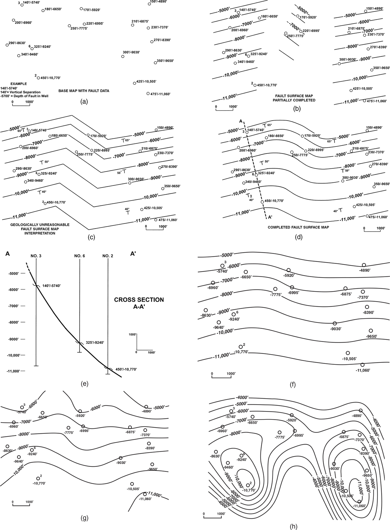
Figure 7-11 (a) Fault surface basemap showing the missing section and depth of the fault in each well. (b) Fault contours established in three areas of well control. Each fault segment is part of the same fault. (c) Unrealistic fault surface interpretation results from connecting each fault segment with straight lines. This is a mechanical approach to contouring. (d) Completed fault surface map using the interpretive form of contouring to reflect the expected geometry of the fault surface. (e) Cross section A-A′ passes directly through Wells No. 3, 6, and 2 and is laid out perpendicular to fault strike. Use of an interpretative approach to contouring results in a gradual, rather than abrupt, change in fault dip with depth. (f) through (h) are computer-contoured maps based on the same fault data as (d). They differ from each other because different gridding algorithms were used: (f) projected slope; (g) closest point; (h) point density.
The well control in this example is located in three separate areas on the basemap. Seven wells are located in the western portion of the map, three in the central portion, and eight to the east. As discussed under the general contouring rules, begin contouring in the area or areas of maximum control. In this case, we first contour the eastern area, where there are eight wells, followed by the western area, with seven points of control, and finally, the central area with three fault cuts. Use a freehand style of contouring or ten-point proportional dividers to initially establish the contour spacing for the map.
Figure 7-11b shows the contours established for the fault in the three areas of well control. Based on the fault data, we assume that the three fault segments are parts of the same fault, so the final step is to extend the contours into the area of no control and connect the fault segments. There are two possible ways to do this. One method is to extend the contours from each segment toward one another as straight lines until they intersect. This method, illustrated in Figure 7-11c, appears to be a more unreasonable or unlikely interpretation. The second and preferred method is to use an interpretive form of contouring (Fig. 7-11d). With this method, some geological license is used in the interpretation to reflect the expected geometry of the fault surface in this tectonic setting. We gradually change the strike direction of the fault connecting the adjacent segments with a smooth curve.
Now that the fault map is complete, we can estimate the dip of the fault at any location. At a depth of around 5000 ft subsea, the dip of the fault is 65 deg, decreasing to 55 deg at 8500 ft subsea, and finally flattening to about 40 deg between −10,000 ft and −11,000 ft. This type of fault shape is common for growth faults (see the Growth Faults section in this chapter). The fault in Figure 7-11d is contoured as a listric (curvilinear concave-upward surface) growth fault; that is, a fault whose dip decreases with depth, whereas the vertical separation or missing section increases with depth.
Figure 7-11e shows a cross section (A-A′) laid out in a northwest-southeast direction perpendicular to the strike of the fault. Three wells lie on the section with fault data for each well posted. An interpretive method of contouring was used to contour the fault surface with depth. This is the preferred method, which provides the most reasonable interpretation. Other methods could have been used, including the mechanical contouring method, in which the dip rate is constant between each pair of well control points but changes at each well. The equal-spaced contouring method also could have been used. Both methods provide a less reasonable interpretation of the fault surface.
Three examples of the same fault data that were contoured by a computer-based mapping program are shown in Figure 7-11f through h. The projected slope gridding algorithm was used for Figure 7-11f. The result is a map similar to the hand-drawn map in Figure 7-11d in that the fault surface is listric but has a smoother curving lateral bend. A least squares gridding algorithm generated a comparable map except that the extrapolated 5000-ft contour did not conform well to the trend of the other contours and the surface was not so smoothly listric. A closest point algorithm was used to generate the fault surface map in Figure 7-11g, resulting in a fault surface that is not geologically reasonable considering the data, which indicate that the fault is a large growth fault. The mapped surface is not listric and the contours are not credible at the limits of the data, both shallow and deep. The closest point algorithm is best suited to a data set with more numerous and more evenly distributed data points than in our example. Lastly, Figure 7-11g is an extreme example of a bogus fault surface map generated by an algorithm (point density) that is unsuitable to the data set. These three examples demonstrate how critical it is to select an appropriate gridding algorithm (including suitable gridding parameters) for generation of a fault surface interpretation or for integration with a structural horizon map.
Comparison to the hand-contoured map in Figure 7-11d indicates that the projected slope algorithm was the best choice among four algorithms to generate the most reasonable fault surface interpretation. But that does not mean the projected slope algorithm is always the most suitable for mapping a listric fault surface with a lateral bend. The best algorithm is dependent on the number and distribution of data points, among other things. Beware of habitually choosing the same gridding algorithm in computer-based mapping. The interpreter must be sufficiently familiar with all the various algorithms and gridding parameters in order to choose the one most suitable to the data set and the geological surfaces in the area of study.
In developing a final fault surface map interpretation, keep in mind that a fault need not remain constant in strike direction, dip, or vertical separation over its entire extent. Along the strike, the vertical separation may increase, decrease, or remain constant, and the strike direction may change. The vertical separation might increase with depth, decrease to zero up-section, or even decrease with depth. A fault may die laterally, have its displacement transferred to other faults or to folds, combine with other faults, or intersect with or terminate against another fault. In areas of salt diapirs, a fault may terminate against salt, extend through it, or even be deformed due to strata draping around the diapir or by salt movement. We again emphasize that a good interpretation of a fault surface must have 3D validity and comply with the tectonic characteristics of the region being mapped, and you must use correct mapping techniques in its construction.
Figures 7-12 and 7-13 are examples of completed fault surface maps. The fault map in Figure 7-12 is that of the “S” Fault in the Indigo Bayou area, Iberville Parish, Louisiana. Although there is some variation in the amount of missing section for this fault, for the most part it appears to be a post-depositional (nongrowth) fault with a vertical separation ranging from 220 ft to 400 ft. The fault exhibits little, if any, growth with depth. This fault surface map is contoured in accordance with the guidelines and rules outlined in this section.
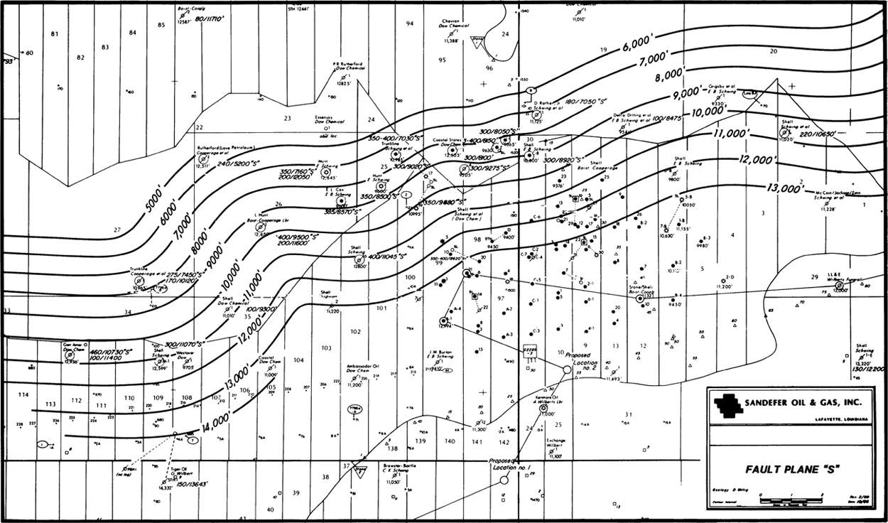
Figure 7-12 Fault surface map on Fault “S” at Indigo Bayou, Iberville Parish, Louisiana. Vertical separation varies slightly from well to well, ranging in size from 220 ft to 400 ft. The fault shows very little change in dip with depth. (Published by permission of Sandefer Oil and Gas, Inc.)

Figure 7-13 Computer-generated fault surface maps of selected normal faults in Ivanhoe Field, U.K. North Sea. Dashed lines indicate that a fault surface extends beyond the contours shown on this map. Wide lines are upthrown fault traces at one horizon. (Modified from Hooper et al. 1992; AAPG©1992, reprinted by permission of the AAPG whose permission is required for further use.)
Contoured fault surfaces of selected normal faults in the Ivanhoe Field, U.K. North Sea, are shown in Figure 7-13 (Hooper et al. 1992). The map is an essential component of a computer-generated set of fault, structure, and isochore maps that were successfully combined in developing more accurate structural and volumetric models of reservoir units than existed at the time. The fault surface maps were used to improve accuracy in determining the intersections of mapped horizons with the faults, and that in turn was the basis for more precise net pay maps. The use of fault surface maps is essential in generating the most accurate maps possible. We present in Chapters 8 and 9 our methodology for integrating fault surface maps with horizon structure maps to generate accurate structure maps, and in Chapter 14 we describe their use in developing the most precise net pay maps.
Types of Fault Patterns
Extensional Faulting
Normal faulting may be defined as motion along a dipping fault surface on which the hanging wall block moves down relative to the footwall block. Normal faults commonly occur as a set with more or less parallel strikes but opposing dips, referred to as a conjugate fault system. Typically, each fault has a different amount of slip, with the fault having the major displacement called the master fault, and the fault with the relatively minor displacement called an antithetic, or compensating, fault. Normal faults are typically steeply dipping; however, the dips of normal faults may range from almost horizontal to vertical. A normal fault typically results in a missing stratigraphic section in electric well logs and a gap on a structure map between the intersections of the fault and the mapped horizon in the upthrown (footwall) and downthrown (hanging wall) fault blocks. This was illustrated in Figures 7-2 and 7-7. Normal faults can be growth (synsedimentary) or nongrowth in nature; can be isolated or display complex patterns; can be virtually planar, listric, or antilistric in profile; can die downward; or can even exhibit deformation.
Extensional basins associated with salt tectonics can have very complex fault patterns. The maximum principal stress axis in extensional basins is vertical, resulting in normal faulting with initial dips of about 60 deg or greater due to extension. Salt masses are commonly associated with crestal grabens, as well as radial and peripheral faulting. Antithetic faults, also referred to as compensating faults, are common in extensional areas.
In addition to single normal faults (structural and growth), there are three principal patterns of normal fault intersections and terminations common in areas of extensional tectonics. These patterns or systems, illustrated in Figures 7-14, 7-17, and 7-20, are (1) bifurcating, (2) compensating, and (3) intersecting. For each of the fault patterns discussed, a fault surface map, one or more cross sections, and a block model are provided to explain and illustrate the pattern.
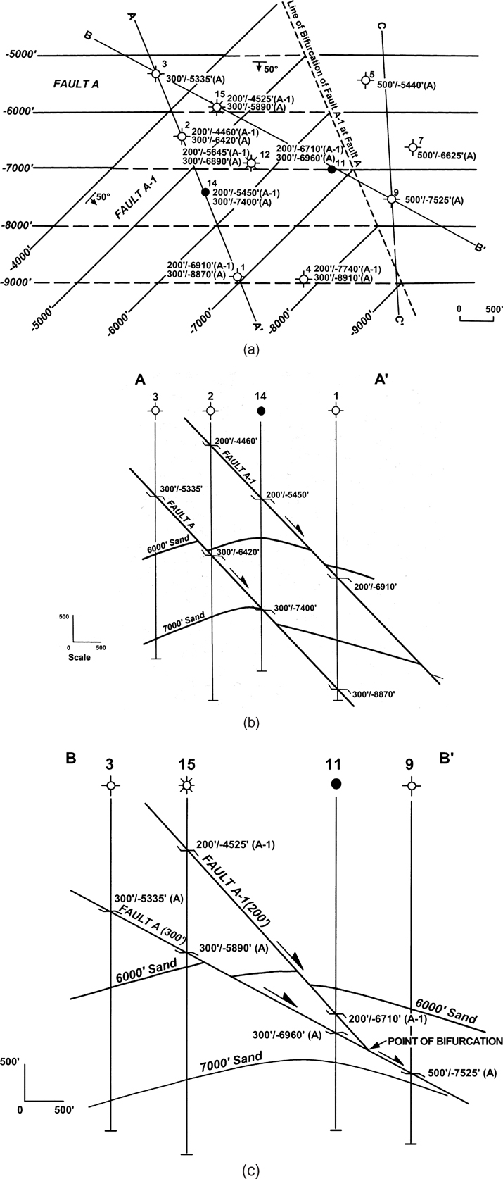
Figure 7-14 (a) Bifurcating fault pattern resulting from two merging faults, dipping in the same general direction. Line of bifurcation indicates where the two faults merge. (b) Cross section A-A′ bisects Faults A and A-1 in such a way that the two faults do not appear on the cross section as merging faults, but instead appear as two parallel faults. (c) Cross section B-B′ is laid out almost perpendicular to Fault A-1 and at an oblique angle to Fault A. In cross section, the faults appear to merge with depth rather than to merge laterally.
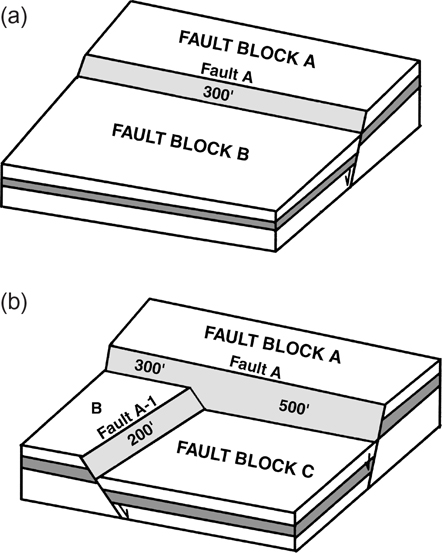
Figure 7-15 Block models show the development of a bifurcating fault pattern. (a) Fault 1 develops with a vertical separation of 300 ft. (b) Fault A-1 develops (vertical separation of 200 ft) and terminates against Fault A. West of the intersection of the two faults, the movement of Fault Block C is accommodated by an additional vertical separation of 200 ft on Fault A.
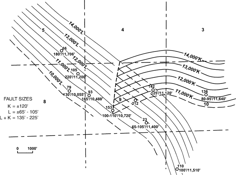
Figure 7-16 Example of a bifurcating fault system. Note the conservation of vertical separation on either side of the line of bifurcation. (Published by permission of Texaco, USA.)

Figure 7-17 (a) Compensating fault pattern resulting from two intersecting faults dipping in generally opposite directions. Line of termination of Fault B at Fault A indicates the intersection of the two faults. (b) Cross section A-A′ illustrates the termination of Fault B at Fault A. Northwest of the intersection, Fault A has a vertical separation of 300 ft, whereas southeast of the intersection, Fault A is 100 ft. Fault B has 200 ft of vertical separation. The vertical separation is conserved across the line of termination.
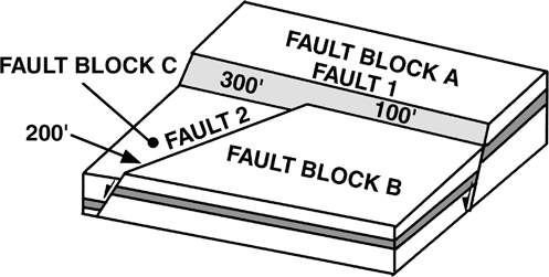
Figure 7-18 Block model of a compensating fault system.
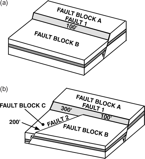
Figure 7-19 Block models show the development of a compensating fault pattern. (a) Fault 1 develops with a vertical separation of 100 ft. (b) Fault 2 develops (vertical separation of 200 ft) and terminates against Fault 1. The portion of Fault 1 west of the intersection of the two faults accommodates the additional 200 ft of movement by Fault Block C, and its vertical separation increases to 300 ft.
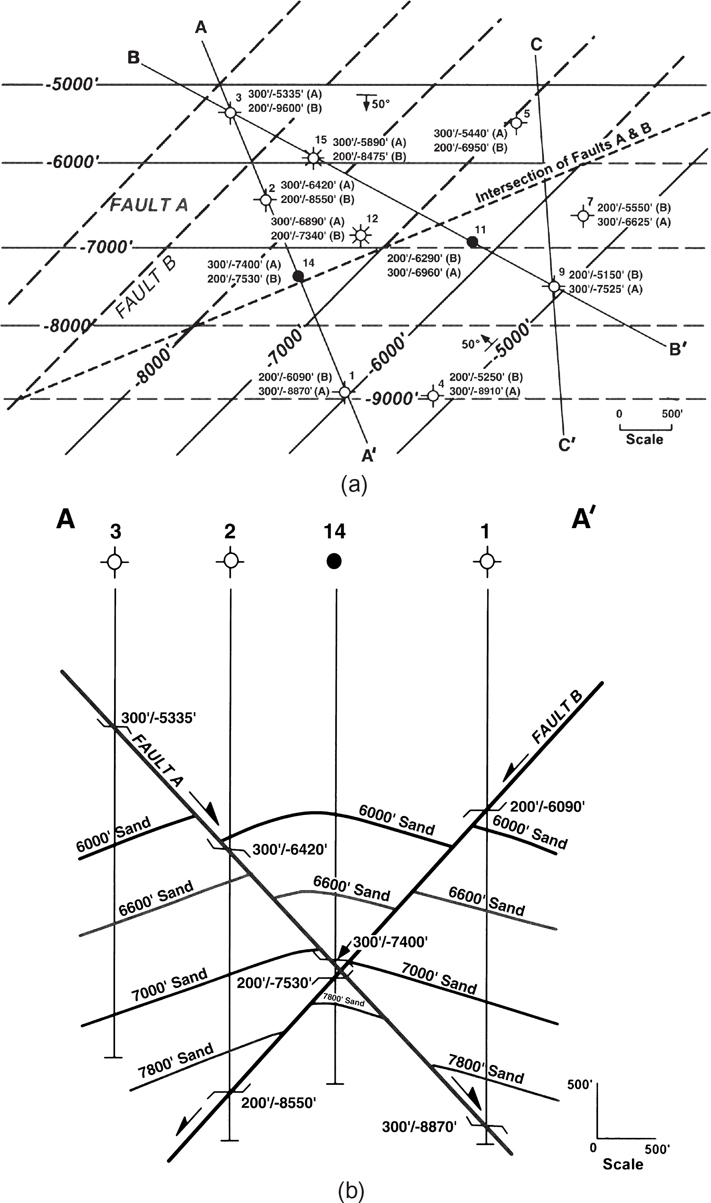
Figure 7-20 (a) Intersecting fault pattern resulting from two faults dipping in opposite directions. Unlike the compensating fault pattern, both faults continue beneath the intersection. This fault map was prepared using the simplified method of assuming neither fault surface is offset. (b) Cross section A-A′ illustrates this intersecting fault pattern. Observe that the faults form a central “graben” block above the intersection and a central “horst” block below the intersection.
Bifurcating Fault Pattern.
A bifurcating fault pattern or system results from two normal faults that dip in the same general direction, as shown in Figure 7-14. The strike direction of each fault is such that the two faults merge laterally in the subsurface and continue on as one fault. The line along which the two faults merge is called the line of bifurcation or intersection. The total vertical separation of the fault across the line of bifurcation must be conserved. This means that the vertical separation of the single fault, where only one fault exists, is equal to or nearly equal to the sum of the vertical separations of the two faults, where two faults are present. The contoured fault surface map in Figure 7-14a shows two intersecting fault surfaces dipping in the same general direction. This interpretation was made using fault data from 11 wells, the contouring guidelines, and an understanding of the geological setting.
Using Figure 7-14, we review the fault system in detail and illustrate the specific characteristics that classify this as a bifurcating fault pattern. Fault A is striking east-west and dipping 50 deg to the south. Fault A-1 is striking northeast-southwest with a dip of 50 deg to the southeast. The two faults are dipping in the same general direction.
Fault A-1 merges with Fault A where the two faults intersect, as indicated by the dashed line of bifurcation. It is the result of the intersection of contours of the same value on the two faults. There are two faults present west of this line. Fault A has a vertical separation of 300 ft, and the vertical separation for Fault A-1 is 200 ft. East of the line of intersection only one fault (Fault A) exists, with a vertical separation of 500 ft. These vertical separation values across the line of bifurcation satisfy the conservation of vertical separation, also referred to as the additive property of faults (see Chapter 8). Notice that the contours for Fault A are dashed west of the line of intersection, indicating that the contour values are deeper than those for Fault A-1. This is a good contouring practice that helps reduce confusion on maps where more than one fault surface is constructed on the same base.
Figure 7-14b and c are two cross sections with a different orientation to the two fault surfaces for each line of section. Remember, cross sections used in conjunction with maps provide another viewing dimension that can be helpful in visualizing the geological picture and solving structural problems. The orientation of the section line, however, is very important. Chosen incorrectly, the line of section can be more confusing then informative.
In the two cross sections through the bifurcating fault pattern, the fault geometry appears different in each section. In cross section A-A′ (Fig. 7-14b), the fault pattern does not appear to be bifurcating. Instead, the two faults appear as parallel faults. Is this real or an optical illusion as a result of the line of section? In Figure 7-14c showing the B-B′ cross section, Fault A-1 appears to merge with Fault A with depth. Real or illusion? Although the two cross sections are geologically and technically correct, they can pose problems for those unfamiliar with fundamental geological principles. When laying out a cross section, be sure to consider the purpose of the cross section and your audience (Chapter 6). As illustrated by Figure 7-14b, a line of section parallel to the line of bifurcation will appear to show two parallel faults. A line of section that crosses the line of bifurcation will show either two faults that merge with depth, as in Figure 7-14c, or a single fault that separates into two faults with depth, as would be illustrated by section C-C′. It is worthwhile to sketch section C-C′ as an exercise to help reinforce this point.
The vertical separation values for the faults have been incorporated into each cross section to represent correctly the offset of the 6000-ft and 7000-ft Sands by Faults A and A-1. The term bed offset means that the horizon has been displaced by the fault, and the displacement is defined in terms of vertical separation. Earlier in this chapter, we showed that the missing section in a wellbore as the direct result of a normal fault is the measurement of the displacement in terms of vertical separation. Since this understanding is very important when preparing cross sections, we detail the procedure for using vertical separation in the preparation of cross sections in Chapter 6. Therefore, in the two cross sections in Figure 7-14b and c, the offset for the beds is constructed using the vertical separation from the wellbore fault data. We cannot overemphasize that wellbore fault data are not throw; therefore, we cannot construct a cross section using the fault data as throw.
Figure 7-15 is a block diagram of a bifurcating fault pattern. A review of Figure 7-15a and b illustrates the geological development of the fault pattern and individual fault blocks. Fault 1 develops first as the rocks fracture and Fault Block B moves downward, creating a fault with 300 ft of vertical separation. Then Fault Block C moves and creates Fault A-1 with a vertical separation of 200 ft. Because Fault A-1 terminates at Fault A, the surface of Fault A to the left of the intersection must accommodate the displacement of Fault Block C. Therefore, the vertical separation increases to 500 ft on Fault A to the left of the intersection. The term bifurcating fault pattern is somewhat unfortunate, as it implies that a single fault splits into two faults. As illustrated by Figure 7-15, this implication is not correct. A bifurcating fault pattern forms when two faults dipping in the same general direction merge to form a single fault, not when one fault splits into two faults.
Figure 7-16 is an example of a bifurcating fault pattern. The fault system shown is that of two faults dipping in the same general direction and merging laterally as indicated by the line of bifurcation. The sum of the vertical separations in the area where two faults are present, east of the line of bifurcation, is equal to or nearly equal to the vertical separation of the one fault west of the intersection.
Fault L dipping to the north-northeast is contoured between −9500 ft and −14,000 ft. The available well control east of the intersection of the two faults indicates that the missing section for Fault L ranges from 65 ft to 105 ft. Fault K, which dips to the north, is contoured between −10,500 ft and −14,000 ft. Based on the well control, the missing section for this fault appears to be about 120 ft. The sum of the vertical separations for Faults K and L east of the line of bifurcation is ±185 ft to 225 ft; west of the bifurcation line, where both faults have laterally merged into one, the vertical separation of Fault L is 165 ft to 225 ft. The nearly equal values for the vertical separation on both sides of the fault intersection show that the vertical separation across the line of bifurcation has generally been conserved.
Compensating Fault Pattern.
A compensating fault pattern or system consists of two normal faults dipping in generally opposite directions toward one another (Fig. 7-17) with an acute angle between the strike directions of the two faults. At the line of intersection, one of the two faults terminates against the other. Conservation of vertical separation is maintained on either side of the line of termination, as demonstrated in the following discussion.
We can look in detail at the example fault surface map for the compensating fault pattern shown in Figure 7-17a. The fault data were obtained from 11 wells. Based on these fault data, the general guidelines presented earlier, and an understanding of the expected fault surface geometry in this setting, two intersecting fault surfaces were contoured as shown.
The completed fault surface map illustrates the specific characteristics that classify this as a compensating fault pattern. Notice that Fault A is striking east-west and dipping to the south with a dip of 50 deg, and Fault B is striking northeast-southwest and dipping at 50 deg to the northwest. The two faults are dipping in generally opposite directions and toward one another. Fault B terminates against Fault A where the two fault surfaces intersect at equal subsea elevations, as indicated by a dashed line referred to as the line of termination.
Southeast of this line of termination are two faults (Faults A and B). Fault A has a vertical separation of 100 ft, and the vertical separation of Fault B is 200 ft. Northwest of the termination line, only Fault A is present and has a vertical separation of 300 ft. These displacement values satisfy the conservation of vertical separation. Therefore, we say that Fault B is compensating with respect to Fault A.
Figure 7-17b is northwest-southeast stick cross section A-A′ shown in plan view on the fault contour map in Figure. 7-17a. The fault data from Wells No. 3, 2, 14, and 1, which lie directly on the cross section, are posted on the section. Fault B terminates against Fault A at a depth of −7460 ft, which corresponds to the point on the fault map (Fig. 7-17a) where the termination line for Fault B intersects the cross section. In the area where Fault A and Fault B are present, Fault A has a vertical separation of 100 ft, and the vertical separation of Fault B is 200 ft. This is shown in Well No. 1 by the fault cut point for Fault A of 100 ft at −8870 ft and 200 ft at−6090 ft for Fault B. Northwest of the termination of Fault B, only Fault A is present with a vertical separation of 300 ft shown in the fault cuts in Wells No. 2, 3, and 14. In Well No. 14, for example, the 300-ft fault cut is at a depth of −7400 ft. The vertical separation values for the faults have been incorporated into the cross section to correctly represent the offset of the 6000-ft and 7000-ft Sands by Faults A and B.
Figure 7-18 is a block diagram of a compensating fault pattern. At times, you may hear the following as an explanation for the fault displacements within a compensating system: “Think of the system in this way. Northwest of the fault intersection, Fault 1 has a missing section of 300 ft. Since Fault 2 is 200 ft, it takes away 200 ft of displacement from Fault 1 southeast of the intersection of the two faults, leaving 100 ft of displacement for Fault 1.” This explanation may provide you with a visual understanding of the missing section for each fault on both sides of the termination line, but technically it is incorrect and can lead to confusion. One fault cannot take displacement away from another fault unless there is active inversion.
Looking at Figure 7-19, think of the geological development of the fault pattern and individual fault blocks in the way they formed. Fault 1 develops as the rocks fracture and Fault Block B moves downward, creating a fault with a vertical separation of 100 ft. Next, Fault Block C moves and creates Fault 2 with a vertical separation of 200 ft. Fault 2 terminates at Fault 1, so Fault 1 to the left of the intersection must accommodate the displacement of Fault Block C. Therefore, the vertical separation increases to 300 ft on Fault 1 to the left of the intersection. Some geologists refer to such movement as a “reactivation of the older fault surface by the younger fault.” If we check for conservation of vertical separation, we see that the 200 ft for Fault 2 plus the initial 100 ft for Fault 1 to the left of the intersection equal the final 300 ft of vertical separation for Fault 1 to the left of the intersection. Comparing Figures 7-15 and 7-19, can you see that the orientation of the younger fault is the only fundamental difference between the bifurcating and compensating fault patterns? For simplicity, we use examples of fault systems in which one fault is implied to be younger. It is also possible that the two faults are contemporaneous.
Intersecting Fault Pattern.
So far, we have discussed two types of fault patterns in which one fault merges or terminates against another fault at their intersection. Now we look at the intersecting fault pattern, which results from two faults (normal or reverse) dipping in such a manner as to intersect in the subsurface; unlike the bifurcating system, in which the two faults merge, or the compensating system, in which one fault terminates against the other, both faults continue downward. The geometric relationship of intersecting faults is very difficult to visualize. Block models can help illustrate this pattern in three dimensions, and 3D seismic data are at times a fantastic data source from which to view these patterns.
Because of the complexity of this fault pattern, a correct interpretation is rarely achieved, even in areas of adequate well and 2D seismic control (Dickinson 1954). When considering the three fault patterns discussed in this section, the intersecting fault pattern presents the most complexities and the solutions are not at all straightforward. With limited available data, a decision must be made whether the intersecting faults formed contemporaneously (Horsfield 1980) or are of two different ages. Without good seismic control, such as a 3D survey, it is often difficult, if not impossible, to determine if the faults formed contemporaneously or at different times. A possible determination is the strike of the two faults. If the material is homogeneous and contains no significant pre-existing discontinuities, then contemporaneous faults will form in response to a single regional stress field, and the strike of these faults may be parallel or subparallel. The strike of normal faults will be perpendicular to the minimum horizontal stress; the strike of reverse faults will be parallel to the minimum horizontal stress. A second hint to whether the faults are contemporaneous is the dip of the faults. Contemporaneous intersecting faults should have the roughly same dip unless the faults have been rotated by subsequent tectonic action.
If the conclusion is that the faults are of two different ages, the next step is to determine which fault formed first and which was second. Such conclusions affect the construction of the fault surface maps, as well as completed structure maps. Today it is frequently possible in areas with good 3D seismic to determine which fault formed first and which was second.
Because of the complexities and uncertainties surrounding this fault pattern, we recommend that the intersecting faults be mapped as if there is no offset of one fault by the other unless the data is adequate to determine which fault is younger and which fault is older. This assumption does result in some error around the intersection of the faults, as even contemporaneous faults do not pass through each other without offset (Ferrill et al. 2000; Ferrill et al. 2009), but it does save time, and the actual interpretation may be impossible to determine from data available. This error extends to any resulting integrated structure map. This compromise should usually introduce less error than an incorrect guess as to the age of faulting. This subject is further discussed in Chapters 8 and 9.
For the intersecting fault example shown in Figure 7-20a, we make one of two assumptions: (1) the faults are contemporaneous, or (2) the relative age of the faults is unknown. With these assumptions, we construct a fault map with both faults meeting at their intersection and continuing downward, unaffected at and past their intersection. The fault maps were prepared using fault data from the 11 wells shown on the map. Fault A is striking east-west and dipping to the south at 50 deg, and Fault B is striking northeast-southwest with a dip of 50 deg to the northwest. The intersection of the two faults is shown as a dashed line. Beneath their intersection, the two faults continue downward with no change in vertical separation. These values are not affected by the intersection of the faults, as they are in the bifurcating and compensating fault systems.
Around the area of fault intersection, a chaotic zone may exist in which both the strata and fault surfaces are disrupted (Ferrill et al. 2000; Ferrill et al. 2009). However, well control and seismic data rarely can identify such disruption and, therefore, the mapping around these intersections is inaccurate. This must be kept in mind when mapping horizons affected by intersecting faults.
The cross section A-A′ shown in Figure 7-20b illustrates the simplified (or compromised) method of preparing the fault surface maps as if the two faults were contemporaneous. Although neither fault surface is offset on the fault map, when the fault surface map is integrated with a structure map, all four resultant fault traces may be offset. This is covered in detail in Chapter 8.
Figure 7-21 is a block diagram of an intersecting fault pattern resulting from two different ages of faulting. Fault 1 developed first, followed by Fault 2. Notice in the figure that Fault 2 cuts through Fault 1, displacing the older fault surface and causing a gap in this displaced surface. Since both faults carry to depth, no change in vertical separation occurs for either fault below their intersection.
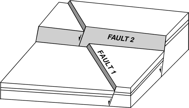
Figure 7-21 Block model of an intersecting fault pattern.
An interpreted seismic line from a 3D survey over an offshore Gulf of Mexico field is shown in Figure 7-22. It shows very clearly an intersecting fault pattern in which both faults appear to pass through one another as if the faulting were contemporaneous, similar to the example used in Figure 7-20. Intersecting faults dipping in generally opposite directions, as shown in the figure, are given the special name intersecting horst-graben faults. Looking at the figure, we can see how this pattern gets its name. Above the fault intersection, the faults form a central graben block; below the intersection is a horst block, thus the name horst-graben fault system.
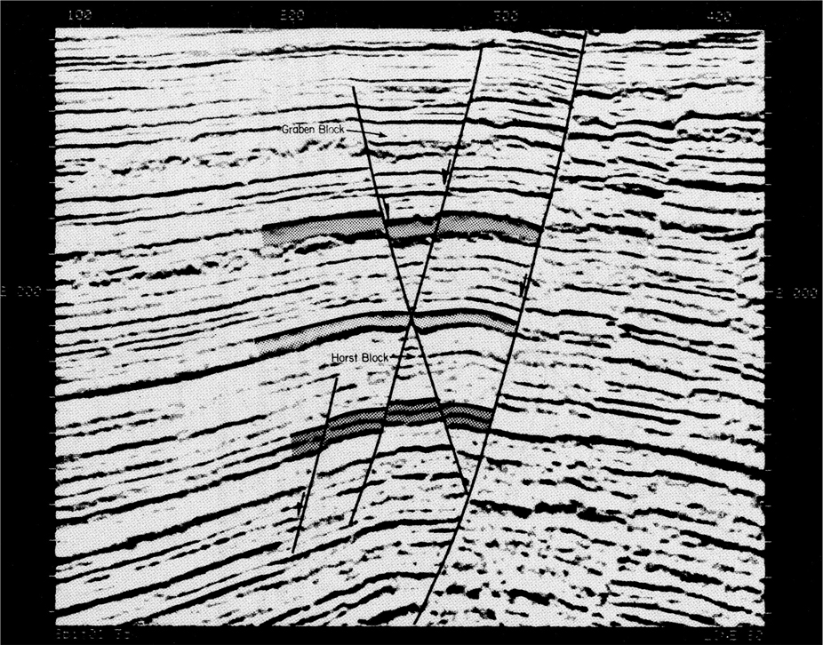
Figure 7-22 Seismic line from a 3D survey shows an intersecting fault pattern. Both faults appear to have formed contemporaneously, since neither fault is offset by the other. Notice that the east-dipping fault intersects and terminates against a second west-dipping fault, forming a compensating fault pattern. (Modified from Tearpock and Harris 1987. Published with permission of Tenneco Oil Company.)
In areas where there is significant seismic data (3D data), it is sometimes possible to determine the relative ages of the faults. If this is possible, fault surface maps can be constructed for both faults, showing displacement of the older fault by the younger one. Integration of these fault maps with structure maps results in a more accurate representation of the fault intersection.
One final note on the different fault patterns: These patterns can be very complex, involving numerous faults in a single area (e.g., Figure 9 in Ferrill et al. 2009). Also, a fault need not remain as one pattern over its lateral or vertical extent. In other words, a fault that is part of a compensating fault pattern in one area can be part of an intersecting or bifurcating pattern in another (see Fig. 7-22).
Combined Vertical Separation.
The term combined vertical separation applies to the relationship that results where two faults of different ages intersect. If a fault surface map similar to Figure 7-20a were constructed for intersecting faults of different ages, the fault surface of the older fault would be offset by the younger fault. The zone of combined vertical separation applies to that segment of the intersecting (younger) fault which lies between the offset surfaces of the displaced (older) fault. This zone is called the “zone of combined throw” by Dickinson (1954); however, his use of the word throw is a substitution for vertical separation.
Figure 7-23a and b illustrate a sequence of faulting involving two normal faults that results in a combined vertical separation. If a well penetrates the area of combined vertical separation, only one of the two intersecting fault surfaces will be crossed (only one fault pick in the well), but the interval shortening or missing section will be equal to the sum of the vertical separations for both faults. The example in Figure 7-23 shows two intersecting faults of different ages dipping in generally opposite directions. The initial Fault 1 has 100 ft of vertical separation. The younger Fault 2, which has 200 ft of vertical separation, has displaced Fault 1 in a manner similar to a fault displacing a horizon. A review of the stratigraphic section in the area affected by both faults, penetrated by Well No. 2 in Figure 7-23b, shows a vertical shortening (or missing section in the well) of 300 ft, which is equal to the combined vertical separation for Faults 1 and 2.
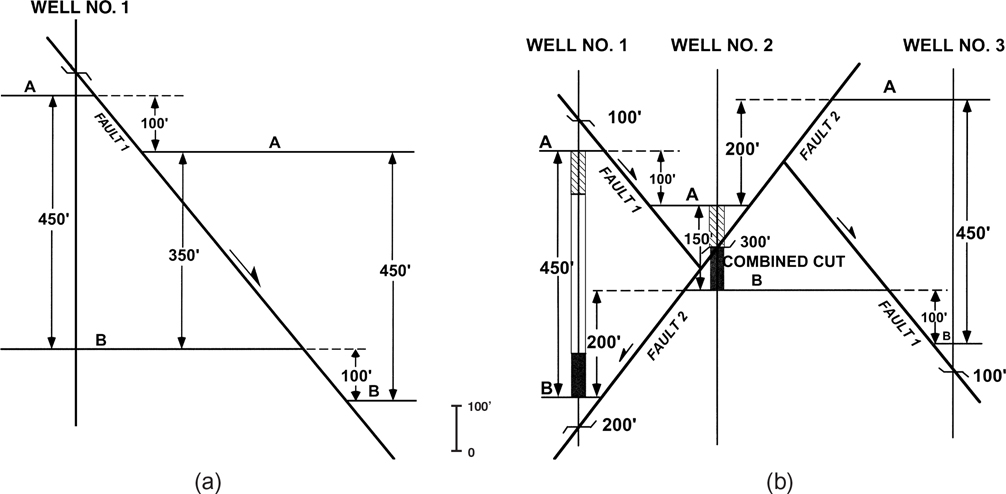
Figure 7-23 Schematic cross sections illustrating the zone of combined vertical separation (zone of combined fault cut), which develops from two intersecting normal faults. (a) Fault 1 with vertical separation of 100 ft. (b) Younger Fault 2, with vertical separation of 200 ft, offsets Fault 1. Well No. 2 penetrates one fault and has 300 ft of missing section. (Published by permission of D. Tearpock and J. Brewton.)
Figure 7-24 is a fault surface map for Fault J. This fault is the north-dipping component of an intersecting fault system composed of two faults of different ages and dipping in opposite directions. The north-dipping fault has a vertical separation of about 80 ft, and the vertical separation of the south-dipping Fault D is about 150 ft. Notice along the line of fault intersection that the fault cuts in Wells No. 2 and 109 are unusually large (235 to 250 ft) compared to the vertical separation of Faults D or J. These two larger fault cuts result from a combined vertical separation.

Figure 7-24 Wells No. 2 and 109 each have combined fault cuts as the result of the intersection of Faults D and J, Golden Meadow Field, Lafourche Parish, Louisiana. (Published by permission of Texaco, USA.)
When working in an extensional area of complex or intersecting faults where an unusually large fault is present in one or more wells, keep the idea of combined vertical separation in mind. An unusually large cut could be the result of a new, previously unrecognized fault, a bifurcating or compensating fault pattern, a buried fault, or a combined vertical separation resulting from intersecting faults of different ages.
The effects of intersecting normal and reverse faults are illustrated in Figure 7-25a through d. The upper part of each figure shows a structure contour map depicting the interruption of a dipping horizon “O” by various combinations of intersecting normal and reverse faults. The cross section in the lower part of each figure shows the structural effects of the intersecting faults on interval “O-P,” which has a constant vertical thickness defined as “c.” Although the vertical separation for the fault in the zone of combined vertical separation is a function of many variables, including horizon dip, fault dip, vertical separation for each fault, and the relative movements of the individual faults, it is usually equal to the algebraic sum of the vertical separation of both faults.
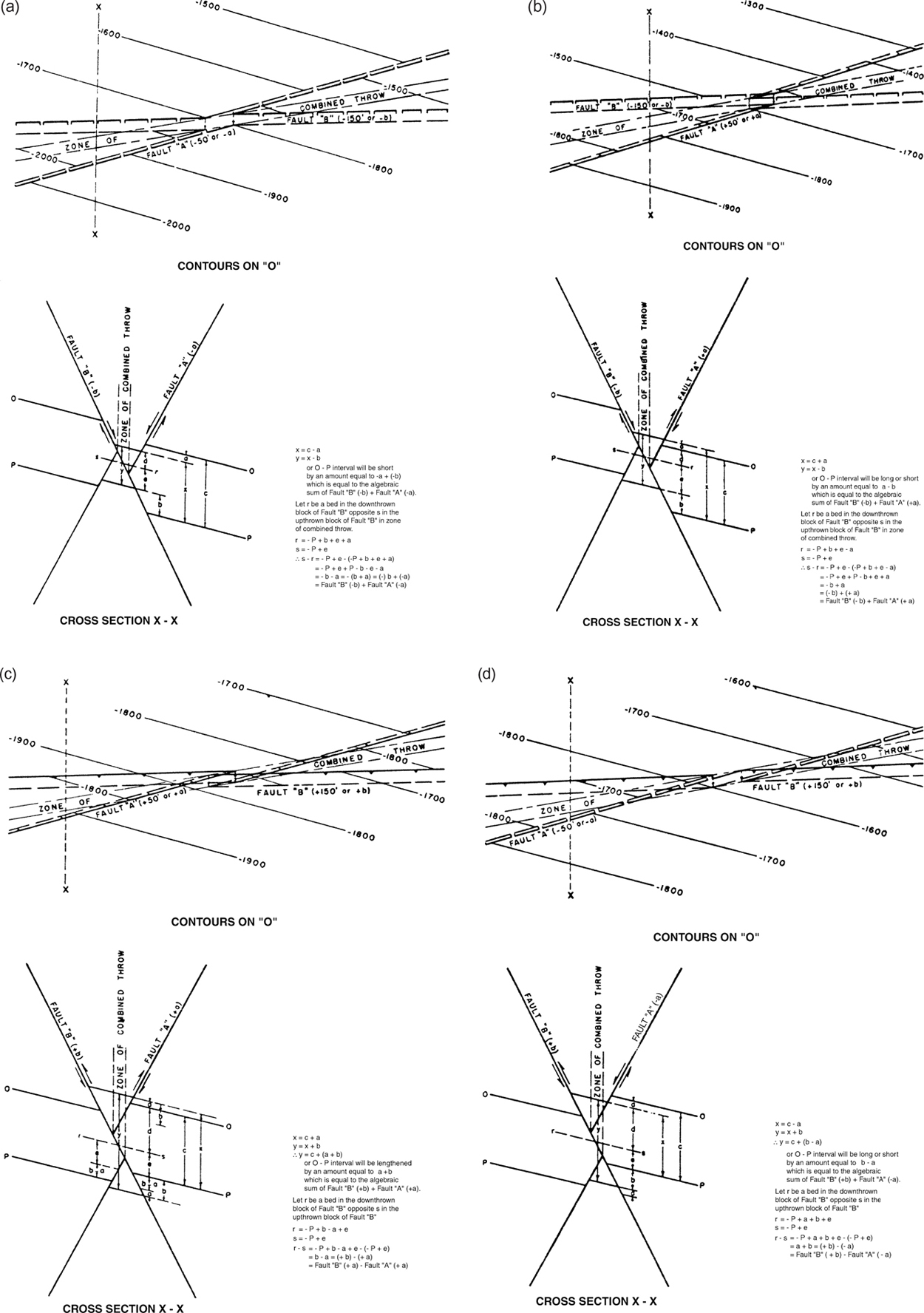
Figure 7-25 (a) Displacement across zone of combined vertical separation (referred to as combined throw by Dickinson [1954]) for intersecting normal faults. (b) Displacement across zone of combined vertical separation for a reverse fault intersected by a normal fault. (c) Displacement across zone of combined vertical separation for intersecting reverse faults. (d) Displacement across zone of combined vertical separation for a normal fault intersected by a reverse fault. (Dickinson 1954; AAPG©1954, reprinted by permission of the AAPG whose permission is required for further use.)
Where the intersecting (younger) fault is normal (Fig. 7-25a and b), the vertical separation of the intersecting fault in the zone of combined vertical separation is equal to the algebraic sum of individual vertical separations; that is, it is equal to (−b) plus (+a). The figures illustrate that where both faults are normal, the vertical separation across the intersected fault in the zone of combined vertical separation will also be normal. Where the intersected fault is reverse, however, the vertical separation will be normal only if the intersecting fault has the greater vertical separation and will be reverse only if the intersected reverse fault has the greater vertical separation (Dickinson 1954).
Figure 7-25c and d show the resulting fault geometry where the intersecting fault is reverse. In these two cases, the vertical separation across the intersecting fault in the zone of combined vertical separation is equal to the algebraic difference between the vertical separations of the intersecting and intersected faults; that is, it equals (+b) minus (+a). The vertical separation across the zone of combined vertical separation will be normal where the intersected fault is reverse and has a vertical separation greater than that of the intersecting fault. Where the intersected fault is reverse and has a vertical separation smaller than that of the intersecting fault, or where it is normal, the vertical separation across the zone of combined vertical separation is always reverse for a reverse intersecting fault. Unlike the geometry involving normal faults where only one fault is seen in the zone of combined vertical separation, the geometry in Figure 7-25c and d results in three faults (i.e., a well in that zone will penetrate three faults).
Compressional Faulting
Reverse faulting is defined as motion along a dipping fault surface on which the hanging wall block rises relative to the footwall block. End members of the reverse fault spectrum consist of vertical and horizontal fault surfaces, as is the case with normal faults. An idealized reverse fault is shown in Figure 7-26. As in Figure 7-2, for normal faults, this figure graphically defines the common fault components used in mapping. Depending on relative amounts of fault and formation dips and wellbore deviation angles, normal faults usually omit section, whereas reverse faults usually repeat section in electric logs. Exceptions occur where the bed dips are near vertical, where wells deviate across the main normal fault may contain repeated section, and a reverse fault can have missing section.
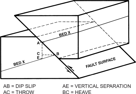
Figure 7-26 Block diagram of Bed X displaced by a reverse fault, showing four different fault components. The front panel is perpendicular to the strike of the fault. (Modified from Tearpock and Harris 1987. Published by permission of Tenneco Oil Company.)
However, in most cases dealing with vertical wells, the terms normal and reverse are in wide use to indicate the presence of missing or repeated section. We should recognize the origin of section omission and repetition during well log correlations and, in doing so, use the genetic terms extensional and compressional faulting. The previous section of this chapter dealt with the practical aspects of extensional faulting. In this section we discuss principles and practical aspects of compressional faulting.
In analogy with Figure 7-1 for normal faults, we derive from the frontal portions of Figure 7-27 a formula for repeated section versus throw (also see Chapter 10 for more complex examples of calculating repeated section with different hanging wall and footwall dips). The formulas are in the dip direction relative to the reverse fault. This formulation applies only to straight reverse fault segments and not curved reverse faults, and here the beds across the fault surface dip at the same angle. Using the trigonometry and equating to the dip slip (S), it follows from Figure 7-27 that
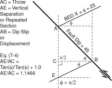
Figure 7-27 Dip cross section used to determine the relationship between repeated section shown by the vertical separation of the bed, which is the vertical line AE, versus the throw (vertical line AC). The AE/AE ratio is calculated from Eq. (7-4). (Published by permission of R. Bischke.)
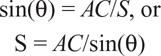
where
S = dip slip = AB
AC = throw
ϕa = apparent bed dip measured in dip direction of fault
θ = fault dip
AE = repeated section or vertical separation (Fig. 7-27; also see Fig. 7-6).
From the law of sines, AC and AE are derived relative to S:
And using trigonometric identities yields and rearranging yields

The AE/AC ratio can be calculated or determined from the repeated section equation Eq. (7-3) or (7-4) or by measured AE/AC with a scale. For Figure 7-27, the calculated AE/AC = 1.1466.
For Figure 7-28, the fault dips to the left and is in a different quadrant. Thus,
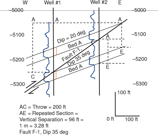
Figure 7-28 Diagrammatic cross section illustrating the relationship between a repeated section in a wellbore and the vertical separation where the beds are dipping in the same direction as the reverse fault. Eq. (7-4) is the formula used for the AE/AC calculation. Compare the relationship in this figure to those shown in Figure 7-27. (Published by permission of R. Bischke.)
For Figure 7-28, using Eq. (7-5), AE/AC = 0.48 and as AC = 200 ft, AE = 96 ft (1 m = 3.28 ft).
In general, our study found that irrespective of the fault dip, either dipping to the left or to the right, if the bed dips in the opposite direction of the fault, then use Eq. (7-4). If the bed dips in the same direction as the fault, then use Eq. (7-5). Measurements of AE/AC can confirm the calculations.
In compressional areas, the determination of fault data begins with well log correlation, just as it does in extensional areas. For a reverse fault, the repeated section, recognized on an electric log by correlation with surrounding well logs, is equal in value to the vertical separation (Tearpock and Harris 1987). Figure 7-28 diagrammatically represents the determination of fault data by the correlation of well logs. This east-west structural cross section is perpendicular to the strike of the fault surface and shows two beds that have been cut by a reverse fault (F-1). At depth, the reverse fault cuts Well No. 1 near −5250 ft and is dipping at an angle of 35 deg to the west, whereas the strata are dipping at 20 deg to the west. By correlation with Well No. 2, the repeated section in Well No. 1 is calculated to be equal to 96 ft and is shown to have completely repeated Bed A in both wells. As shown in the cross section, the throw of Fault F-1 is represented by the vertical line AC, which is equal to 200 ft. Vertical separation, represented by the vertical line AE, is equal to the repeated section, which is 96 ft. This correlation example demonstrates that the repeated section obtained for the fault due to a reverse fault is equal to vertical separation. Notice, however, that the throw is not determined at Well No. 2, but rather from an accurately drawn cross section constructed from Wells No.1 and No. 2 along with the bed and fault dips.
In summary, Figure 10-28 shows a cross section with two wells, each of which has intersected reverse Fault F-1. The fault and beds are dipping in the same direction. By log correlation, we see that the repeated section in each well is equal to 100 ft, which is the vertical separation (AE). Unlike the first example in Figure 7-27, in which the throw was about one-half the size of the vertical separation, here a measurement of throw reveals it to be over twice as large as the vertical separation. Once again, we diagrammatically show that the throw of Fault F-1 cannot be measured accurately by log correlation alone but by cross section, and also that the throw is not equal to the repeated section.
Thrust faults are dip-slip faults in which the hanging wall has moved up relative to the footwall. Isolated thrust faults generally dip less than 30 deg during active slip and commonly dip between 10 and 20 deg at their time of formation (Suppe 1985). Many thrust faults lie along bedding planes over part of their length.
Thrust faults develop in two primary settings: (1) compressional plate boundaries and (2) secondary faulting in response to folding. The foreland of fold-and-thrust belts have been the most extensively studied areas of thrust faulting because of significant potential for both petroleum and coal reserves. There are two basic types of fold-and-thrust belts: (1) those dominated by thrust faulting such as the southern Appalachians and the Cordilleran belt in western Canada and the United States, and (2) fold-dominated belts such as the central Appalachians and Jura mountains of Switzerland (Suppe 1985).
Individual thrust faults commonly cut up the stratigraphic section in a sequence of discrete crosscutting segments called ramps and flats. The thrust fault separates the deformed hanging wall structure from the substrate along a bedding plane zone called a decollement (from the French word meaning “unglue”). Thrust and reverse faults, as with normal faults, can bifurcate in the ramp areas with total displacement distributed among the many fault splays and also absorbed in folds. In many cases the hanging wall blocks of thrust faults are folded; this results from bending of the fault blocks as they slip over nonplanar fault surfaces. These folds are called fault bend folds (Suppe 1985). The best-known fault bend folds are those associated with the stepping-up of thrust faults from lower to higher decollement surfaces.
Three names are commonly applied to compressional faults: (1) high-angle thrust faults, usually referred to as reverse faults (steeply dipping), (2) low-angle thrust faults (moderately dipping, sometimes defined as less than 45 deg of dip), and (3) overthrust faults (very shallow dip, usually with long horizontal transport).
How do we map the surface of a reverse fault? Most of the fault surface map and cross-section techniques already described for extensional faulting apply to compressional fault surface mapping. For the most part, the differences lie in the complexities of the compressional fault patterns and the limit of good-quality well and seismic data. Probably more than in any other tectonic setting, we must have a thorough understanding of the principles of structural geology and the structural styles at play, and we must be able to think and visualize in three dimensions.
Single Compressional Faults.
Figure 7-29 is an example of a single compressional reverse fault surface map. The interpreted fault surface is based on data from seven wells. The techniques used to construct the fault surface map are the same as those used for normal faults. Notice in this example that the depth for each fault cut is expressed as a positive number (300 ft/5245 ft). This means that these fault picks are above sea level. The vertical separation of 300 ft refers to the vertical thickness of the repeated section.
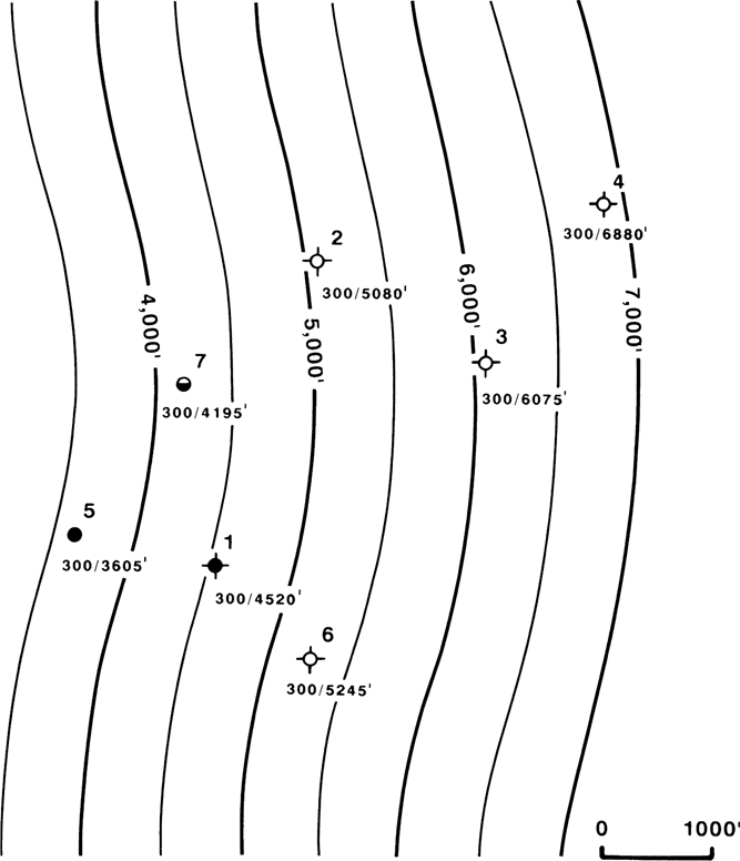
Figure 7-29 Fault surface map for a reverse fault with a vertical separation (repeated section) of 300 ft.
Intersecting Compressional Faults.
A compressional fault pattern of two reverse faults dipping in the same general direction is shown in Figure 7-30a. The data from 12 wells, the general guidelines presented earlier, and an understanding of the compressional tectonic setting were used to construct the fault surface map interpretation for the two reverse faults A and B. Fault A is striking east-west and dipping to the south at 35 deg, and Fault B is striking northeast-southwest and dipping 35 deg to the southeast. The two faults merge laterally as indicated by the dashed line of intersection. We can see by reviewing the fault surface map that the vertical separation is conserved across the line of intersection; this means that the combined vertical separations for Fault A (125 ft) and Fault B (150 ft) west of this line equal the vertical separation of Fault A (275 ft) east of the intersection.
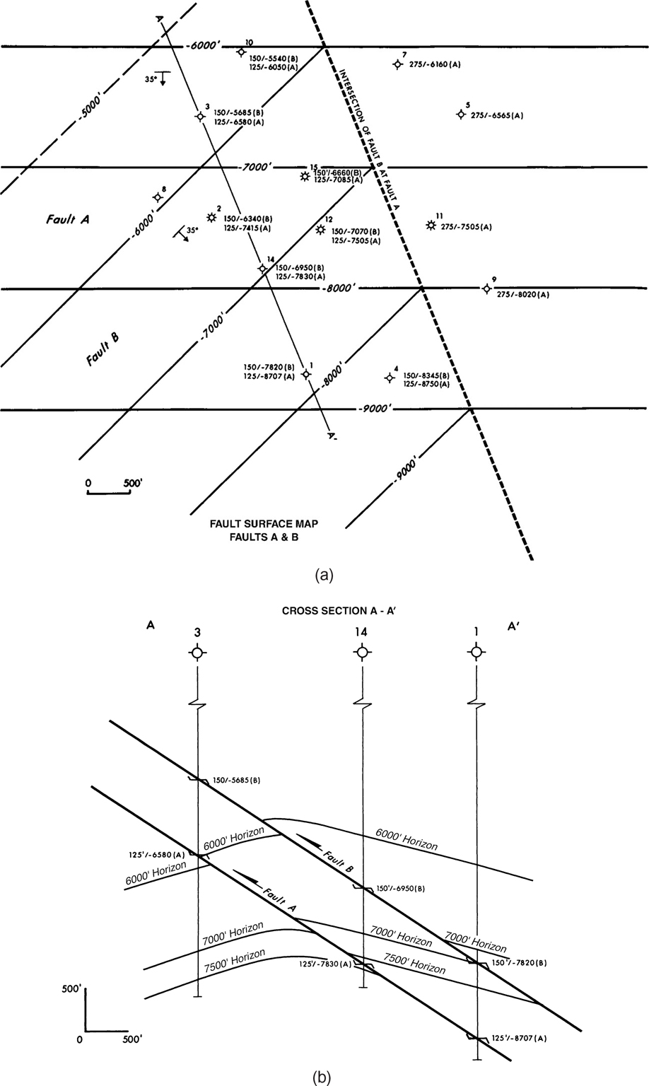
Figure 7-30 (a) Fault surface map of two intersecting reverse faults. (b) Cross section A-A′ crosses the two faults at an orientation that makes the two intersecting reverse faults appear to be parallel.
The change in displacement for these reverse faults across the intersection line is the result of their intersection. Do not mistake the change in displacement in this example with changes in fault displacement resulting from its transfer from one structure to another. In other words, this example is not related to what Dahlstrom (1969) refers to as the compensatory mechanism for reverse faults (thrusts) wherein fault displacement that is diminishing in one fault is replaced by increasing displacement on an echelon fault. Those displacement changes occur in a transfer zone and result from all the associated faults being rooted in a common sole fault. This type of faulting and change in displacement is discussed in Chapter 10.
Figure 7-30b shows cross section A-A′. The displacement for each fault has been incorporated into the offset of each stratum shown on the cross section. Remember, just as in the extensional faulting examples, the displacement of the strata is described in terms of vertical separation. Therefore, the footwall and hanging wall intersections for each stratum with Faults A and B are constructed with the vertical separation technique used to displace a stratum correctly from one fault block to another in cross section. This is the same technique used to construct the cross sections for the extensional and compressional fault patterns, which was introduced in Chapter 6.
Ramp and Flat Thrust Faults.
Ramp and flat fault surfaces develop such that the fault surface moves subparallel to bedding in incompetent strata and ramps to higher structural levels in competent rock. If the ramp intersects another incompetent rock layer, then the ramp may transform again into another flat. This geometry is illustrated in Figure 7-31. Figure 7-31a is a fault surface map of an idealized ramp and flat thrust fault. As with all fault surface maps, the interpretive method of contouring is recommended. This gives you the geological license to construct the fault surface map to reflect the expected geometry in the area of study.
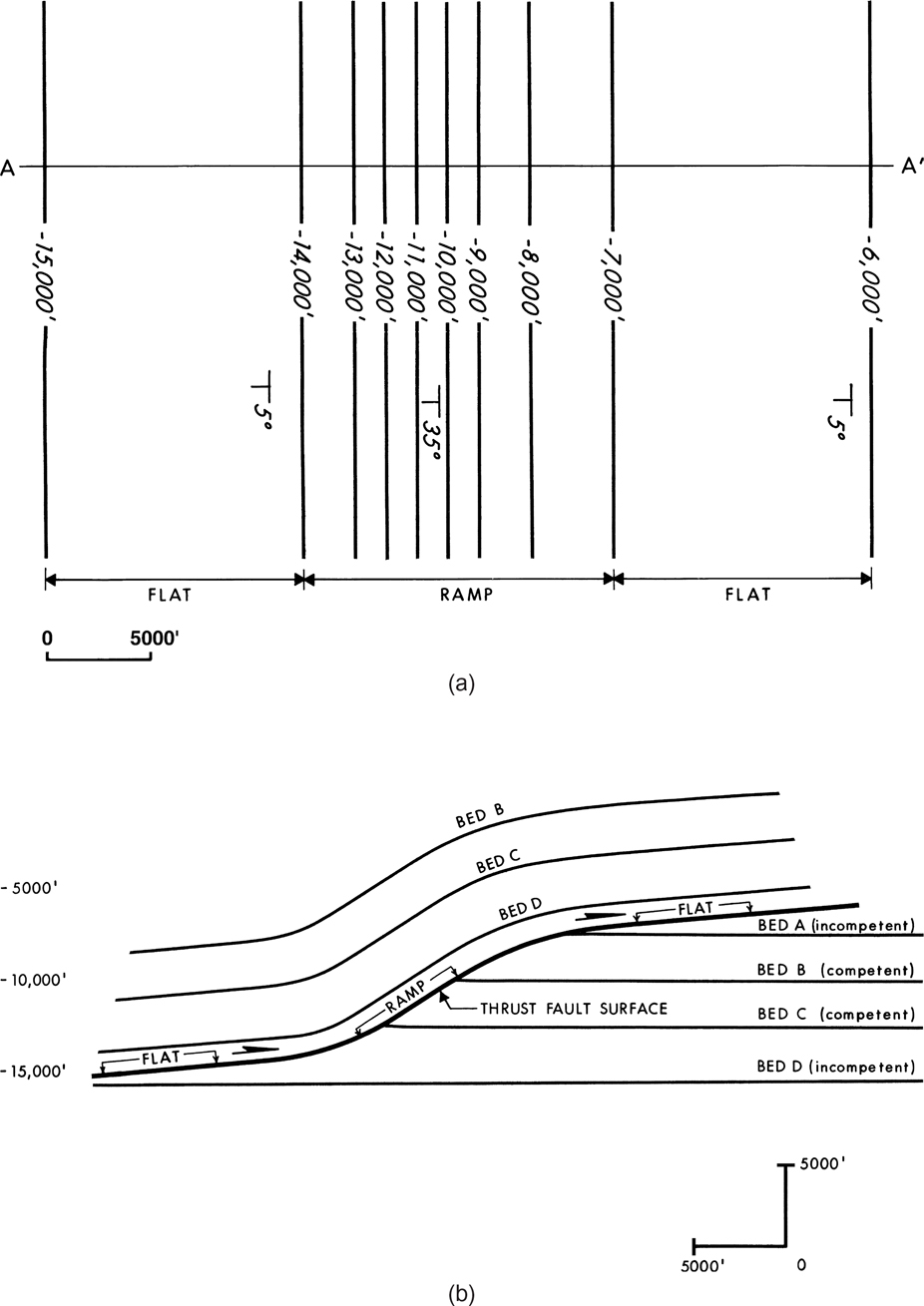
Figure 7-31 (a) Fault surface map for an idealized ramp and flat thrust fault. (b) Diagrammatic cross section, parallel to the transport direction of the thrust fault shown in Figure 7-31a.
Figure 7-31b is cross section A-A′, which shows the fault surface and the disrupted beds. Notice how the strata in the hanging wall are thrust up and over the same strata in the footwall. The geometry of these faults is detailed in Chapter 10.
A fault surface map of the Absaroka thrust fault in the Fossil Basin of Utah and Wyoming is shown in Figure 7-32. Twenty oil and gas fields have been found in the hanging wall block of the Absaroka thrust fault in the southern Fossil Basin. The fault surface map in general reflects a steep ramp to the west from about −20,000 ft to −12,000 ft, a flattening or gentle rise in the central portion of the fault map between −12,000 ft and −5000 ft, and then another steepening ramp to the east (Lamerson 1982).
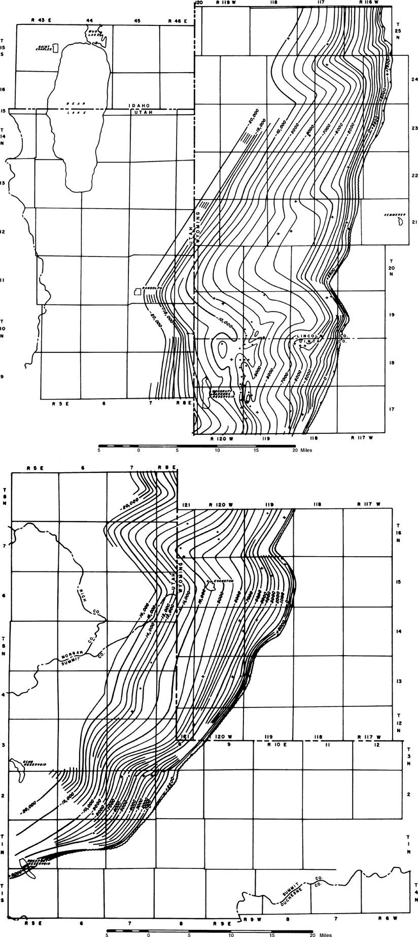
Figure 7-32 Fault surface map of the Absaroka thrust fault in the Fossil Basin of Utah and Wyoming. Note the changes in fault dip from east to west. (From Lamerson 1982. Published by permission of the Rocky Mountain Association of Geologists.)
A portion of the Hogsback ramp and flat thrust fault is shown in cross-sectional view in Figure 7-33. This cross section clearly illustrates the features of the ramp and flat portions of this type of thrust fault. Observe that the flat parallels the Cambrian rocks, which serve as the zone of weakness for the basal detachment zone. As the Hogsback thrust fault cuts up-section across Paleozoic and Mesozoic rocks in the footwall, it creates a ramp with west dip of 20 to 30 deg in the hanging wall rocks of the thrust.
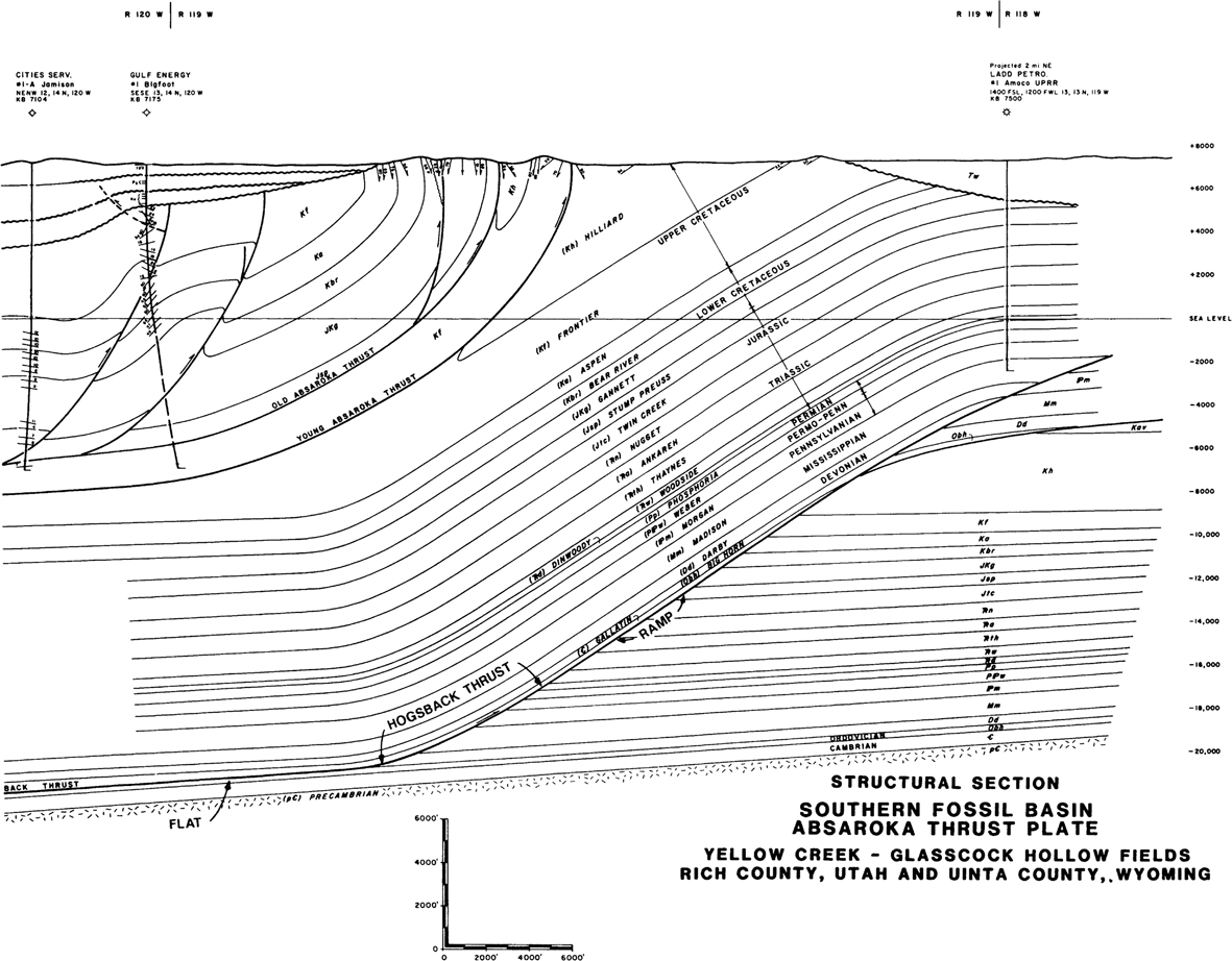
Figure 7-33 Cross section illustrating the geometry of the Hogsback ramp and flat thrust fault. (Lamerson 1982. Published by permission of the Rocky Mountain Association of Geologists.)
Fault surface mapping is not commonly done in compressional areas, although there is no reason why it should not be used and, indeed, it is often required to aid the understanding of complex thrust fault geometry. Hydrocarbon traps are not common along thrust faults, but instead the anticlines that form in the hanging wall blocks act as the primary trapping mechanism. These structural anticlines are often sufficient for trap delineation with little, if any, fault interaction. We strongly believe, however, that the mapping of faults is an integral part of any geological study regardless of the tectonic setting and can significantly add to the understanding of the geology.
Figure 7-34a is the fault surface map for the Aguaclara ramp and flat thrust fault from the southeastern thrust front of the Eastern Condillera of Colombia, South America (Rowan and Linares 2000). This fault surface interpretation and map were generated from both well log and seismic data. The fault surface in this case is mapped in time (msec) rather than depth. Observe the classical ramp, flat, ramp geometry of the fault surface. One of the seismic sections used in this interpretation is shown in Figure 7-34b. Observe how the hanging wall beds have been folded due to the effects of thrust faulting.

Figure 7-34 (a) Fault surface map for the Aguaclara ramp and flat thrust fault, Colombia. Contour interval is 400 msec, relative to an arbitrary datum near the surface. (b) Interpreted seismic profile; location shown in (a). Solid lines are axial surfaces. (Modified after Rowan and Linares 2000. AAPG©2000, reprinted by permission of the AAPG whose permission is required for further use.)
Fault Data Determined from Seismic Information
Up to this point, most of the information reviewed on fault surface mapping has related primarily to fault data determined from well logs and the use of these data. Seismic data can also provide valuable fault information to aid the mapping process, as shown in Figure 7-35. This section covers some basic techniques for integration of fault data determined from seismic sections with data obtained from well control.

Figure 7-35 Illustration of the usefulness of fault-tying in propagating a fault surface over a series of seismic lines. The lower diagram is a map of the fault pattern at the level of Bed A. (Prepared by C. Harmon. From Tearpock and Harris 1987. Published by permission of Tenneco Oil Company.)
First, we make a few assumptions with regard to the seismic data being used to assist in mapping fault surfaces. These assumptions are as follows:
The data being used are of reasonable quality and have been correctly processed up to and including migration of the data.
The two-way time-to-depth conversion is known (i.e., a reliable velocity function exists) and does not vary significantly across the area being mapped.
The lines have been interpreted correctly, with all faults tied at line intersections. In areas of complex structures, this may not be possible. Where 2D data are used, steep dips pose difficulties due to the migration mis-tie between strike and dip lines. In these cases, you may have to rely mostly on the dip-oriented lines. This sort of problem makes fault surface mapping a very helpful tool in identifying faults on successive dip lines (Chapters 5 and 9).
If these assumptions are met, seismic data can provide three very useful types of fault information that aid in the integration of fault data from wells to generate a fault surface interpretation and map. First, seismic data offers a method of establishing a fault identification (ID). Second, it provides the location of a fault surface in space. Third, the amount of vertical separation for a fault can be measured.
The tying process provides us with a method of establishing a fault ID. In short, by tying a fault on a series of lines, we can be sure that the fault seen on various lines is formed by the same fault surface. A fault interpretation that does not tie between lines cannot be correct. Merely tying the faults, however, does not ensure that the fault interpretation is valid, since any nonvertical surface can be tied between a series of lines. To establish validity, a fault surface map must be constructed to confirm that both the fault dip and the changes in strike of fault contours are geologically reasonable.
Seismic data offer a method of visualizing a fault interpretation through a series of lines. By tying the fault traces from these seismic sections, we can be assured that a given fault seen on one section is the same fault seen on other profiles. A schematic illustration of this is shown in Figure 7-35.
Seismic data give us a location of the fault surface in space, and unlike well data, data from seismic sections are over a series of points along the profile of the line. This enables us to map fault surfaces over a greater area and in areas where no well control exists.
It is important to remember that accuracy of points plotted from seismic data is dependent on the accuracy (appropriateness) of the velocity function used to convert seismic time to a depth value. Figure 7-36 illustrates what influence a velocity function can have on dipping surfaces. The figure shows two positions for a proposed directional well plotted on a seismic line based on two different velocity functions. Both functions are possibly valid for this prospect. As the illustration shows, the use of the slow velocity function places the directional well in the upthrown fault block; however, the fast function places the well in the downthrown fault block. The upthrown block is the target block to test horizons 1 and 2. The use of the wrong velocity would cause the exploratory well to be drilled in the wrong fault block. In this particular situation, since the correct velocity was not known, a straight hole design was chosen rather than risk missing the prospective fault block with a directional well. The same problem can apply to fault interpretations. In some cases, there may be some uncertainty as to the two-way seismic time corresponding to a particular depth. If the position of a fault is especially critical, error bars can be placed around a posted point that will graphically illustrate spatial uncertainty for a particular datum.
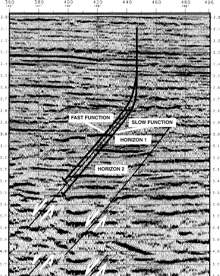
Figure 7-36 Seismic section shows the effect of velocity function uncertainty on the location of a directional well. (Prepared by C. Harmon. Modified from Tearpock and Harris 1987. Published by permission of Tenneco Oil Company.)
The third type of information seismic data can provide is a measurement of the vertical separation of a fault. There is often disagreement between geologists and geophysicists with regard to the amount of missing or repeated section for a fault estimated from well log correlation as compared to that estimated from a seismic section. In many cases, the difference between what the geophysicist is calling displacement and what the geologist is calling displacement is the result of a misunderstanding of fault component terminology. If we assume the vertical resolution limitation of seismic data is known, then the answer to this discrepancy is that two different values for displacement are being measured. As discussed earlier in this chapter, the amount of missing section determined from correlation of an electric log of a well is not equal to throw, but rather, equal to vertical separation (unless, of course, the strata in the area have zero dip or the fault is vertical). Then the values for throw and vertical separation are the same. What is commonly measured on a seismic line for fault displacement is not vertical separation but throw and, more commonly, apparent throw, which is a measurement of fault displacement dependent on the orientation of the seismic line in relation to both the strata and fault dip. The only case where we can actually measure the true throw of a fault, at a particular depth, is where the seismic line is oriented perpendicular to the strike of the fault surface (not perpendicular to the fault trace as seen on a structural map). This means that if several seismic lines, oriented at different angles to the strike of a fault surface, are used to estimate the throw of that fault, each line will yield a different value for the apparent throw for the same fault. Even if it were possible to shoot all seismic lines perpendicular to the strike of each fault surface being mapped, the throw of the fault is not the fault component used in the construction of fault and integrated structure maps, and it is not the displacement value determined from well logs. The added work and expense does not seem justified.
Fault displacement problems from seismic data can be easily reconciled by estimating the vertical separation of a fault from seismic lines, instead of throw or apparent throw. If a seismic line has good correlations across a fault, it is very simple to measure the vertical separation for that fault. Remember, the amount of missing section for a fault in a well log is the measurement of the fault’s vertical separation. In order not to confuse components in our fault displacement measurements and constructed maps, the vertical separation for a fault is a required measurement on a seismic section. These depth-converted vertical separation values can then be used to tie the fault data from wells and aid in the construction of the fault and structure maps.
Figure 7-37 illustrates the proper method for measuring the vertical separation from a seismic line. The line is an east-west line shot in the central Gulf of Mexico Basin by TGS Offshore Geophysical Company. It is an excellent line to use to define the procedure for measuring vertical separation because the dip of the structure changes from east to west. At the eastern end of the line, the structure is essentially flat, with zero dip; to the west, the dip increases. Therefore, we can show the procedure for measuring the vertical separation in flat-lying beds as well as those with significant dip. We also show the comparison of the values for vertical separation and apparent throw to reinforce the understanding that these fault components are not the same and that the use of throw in place of vertical separation can cause significant mapping errors.
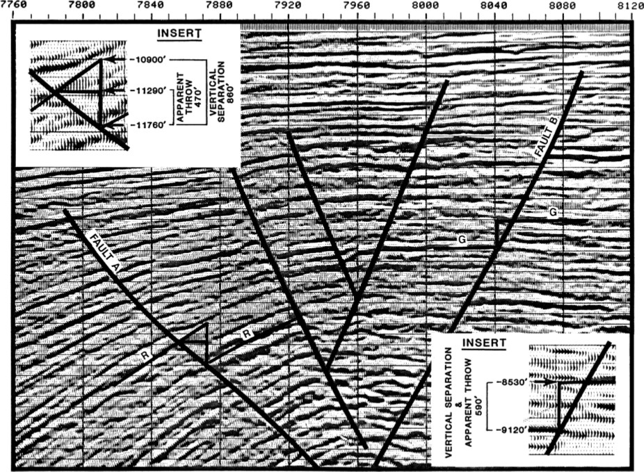
Figure 7-37 Seismic line offshore Gulf of Mexico. The figure inserts illustrate the correct method for estimating the vertical separation of a fault from a seismic line where the events are dipping (Horizon R) and where the events are horizontal (Horizon G). In order to contour the correct displacement, based on seismic data, across a fault, the vertical separation must be estimated. Throw is not used in subsurface mapping. (Modified from Tearpock and Harris 1987. Published by permission of TGS Offshore Geophysical Company and Tenneco Oil Company.)
We begin with the displacement for Fault A at Horizon R. The procedure is more easily followed by using the insert blowup in the upper left corner of the figure. Horizon R is dipping at about 16 deg (depth-corrected) to the west. To measure the displacement of the fault in terms of vertical separation, project the dip of the horizon from the upthrown fault block through the fault, as if the fault were not there, into the downthrown block until the projection is vertically over the intersection of Horizon R with the fault in the downthrown block. Then convert time to depth. The vertical difference in depth from the projection, at −10,900 ft, to the downthrown intersection of the horizon and fault, at −11,760 ft, is 860 ft. This is the measurement of the vertical separation of the fault at this horizon. If a well were drilled through the fault at shotpoint 7865, so that Horizon R is faulted out of the well, the missing section in the well log would be approximately 860 ft.
The measurement of the apparent throw of the fault at this horizon is the vertical difference in depth from the intersection of Horizon R with the fault in the upthrown fault block (−11,290 ft) to the intersection of the horizon with the fault in the downthrown block (−11,760 ft), and this is 470 feet. The difference between the apparent throw and the vertical separation of the fault at Horizon R is a significant 390 ft.
Turning to the right side of the figure, we conduct the same procedure and measure the displacement of Horizon G by Fault B, in an area in which the structural bed dip is essentially zero deg. Refer to the insert blowup in the lower right corner of the figure. First, measure the vertical separation by projecting the dip of the horizon in the upthrown block through the fault into the downthrown block until the projection is vertically directly over the intersection of Horizon G with the fault in the downthrown block. The vertical distance between the depth of Horizon G at the fault intersection in the upthrown block at −8530 ft, and the depth of the horizon/fault intersection in the downthrown block, of −9120 ft, is 590 ft.
The apparent throw, measured as the vertical distance from the intersection of the horizon with the fault in the upthrown block to the intersection of the same horizon and fault in the downthrown block, is 590 ft. This is the same value obtained for the vertical separation. Since the strata dip at this location is zero deg, we should expect these values to be the same, based on the definitions and discussion presented so far in this chapter.
If necessary, go back and review these procedures until you thoroughly understand how to measure the vertical separation and clearly see how it differs from apparent throw. It is essential to remember that whether the fault data are derived from well logs or seismic lines, the same fault component for displacement must be used in mapping faults and structures, and that component is vertical separation. Of course, vertical separation changes laterally along a fault and varies with depth, so you need to determine it on an appropriate number of seismic sections at depths suitable for the mappable horizons.
Figure 7-38 illustrates the accuracy of the technique outlined above in reconciling well log data with seismic data. The seismic line is a Tenneco Oil Company line in South Marsh Island (SMI), offshore Gulf of Mexico. The seismic line intersects the Signal Well No. 1 in SMI Block 67. A fault in the Signal Well produces a missing section equal to 720 ft at a log depth of 10,940 ft, and it faults out Horizon A. Based on this seismic line, the apparent throw of the fault at Horizon A, marked on the line, is 505 ft, and the vertical separation is 695 ft. Notice that the measurement for the vertical separation agrees very closely with the missing section of 720 ft obtained in the well. The estimate of the apparent throw, however, differs by nearly 200 ft from the estimate of fault displacement by well log correlation. By this example, we again illustrate the importance of measuring the same fault component to obtain the value for fault displacement, which will later be used for fault and structure mapping, whether that value is derived from well log or seismic data.
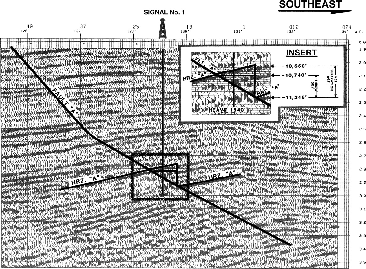
Figure 7-38 Seismic section illustrates the accuracy with which the vertical separation can be estimated, as compared to fault data from a well log directly on the section line. The missing section is 720 ft in the Signal No. 1 Well by correlation with surrounding wells. This compares favorably with the vertical separation of 695 ft estimated from the seismic section. The apparent throw of the fault is only 505 ft. (From Tearpock and Harris 1987. Published by permission of Tenneco Oil Company.)
Seismic and Well Log Data Integration—Fault Surface Map Construction
Since the measurement of fault displacement data can be made from seismic and well log data, both can be used in the construction of fault surface maps. Figure 7-39 illustrates the integration of fault data from two well logs and two seismic lines to construct a fault surface map. The fault data obtained from the well logs are posted next to the appropriate well, and the fault data from the two seismic lines are posted next to the shotpoints at which the data were obtained. Unlike fault data from a well log, which provides fault information from a single depth at a specific location, a seismic line presents continuous fault data over a series of shotpoints along the profile of the line. This permits the fault surface to be mapped over a greater area than would be possible with well log data alone. The seismic also provides a tie to each well to confirm whether the fault cut observed in the well is the same fault surface seen on the seismic line.
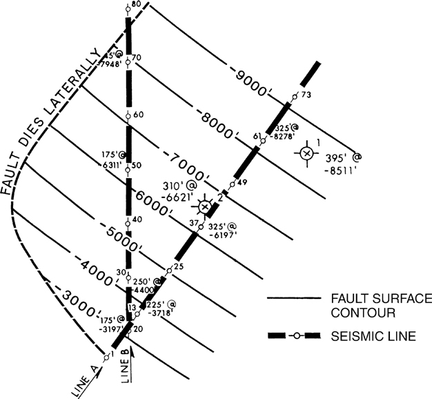
Figure 7-39 Fault surface map prepared using data from well logs and seismic sections. (Modified from Tearpock and Harris 1987. Published by permission of Tenneco Oil Company.)
Fault-Displacement Mapping.
A review of each fault surface map presented in this text reveals that the vertical separation and subsea depth for each well log or seismic fault pick is posted on the basemaps (e.g., 310 ft/−6621 ft). So far, we have used only the subsea depth data to prepare fault surface contour maps. What about the posted vertical separation data? Can these data be used for mapping and, if so, what is their importance? The vertical separation of the fault can and should be contoured where sufficient data are available. Such a map, called a vertical separation map, or throw map by some, provides additional information on the growth history of the fault and additional data for the construction of integrated structure maps (see Chapter 8).
In Figure 7-40a, vertical separation contours are superimposed on the fault surface contours. This vertical separation is contoured in a dashed pattern with a contour interval of 200 ft. Notice that the vertical separation contours are perpendicular to the fault surface contours at depths greater than −5000 ft. This type pattern indicates that the fault is post-depositional and is therefore termed a structural (nongrowth) fault. In other words, the fault is not a syndepositional growth fault; it does not show an increase in displacement with depth. However, the deviation in trend of the vertical separation contours, at a depth from about −3000 ft to −5000 ft, shows an increase in vertical separation with depth and indicates the time during which the fault was active.
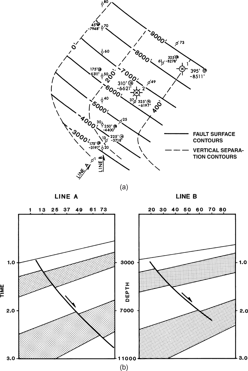
Figure 7-40 (a) Vertical separation contours added to fault surface contour map provide additional information that is helpful during fault and structure map integration (see Chapter 8). (Modified from Tearpock and Harris 1987. Published by permission of Tenneco Oil Company.) (b) Seismic lines A and B shown in map view in Figure 7-40a. (From Tearpock and Harris 1987. Published by permission of Tenneco Oil Company.)
This information has application in evaluating a fault trap because it graphically illustrates the depth of the geological interval affected by post-depositional faulting. A late trap formed by a post-depositional fault can be evaluated as a prospect as long as migration of hydrocarbons occurred during or after the initiation of fault movement. Displacement mapping for growth faults is also very important and is covered later in this chapter.
Seismic Pitfalls
As we have already mentioned, this text is not intended to instruct in all areas of seismic interpretation, nor is there any intent to discuss in detail the pitfalls of seismic interpretation. However, several seismic pitfalls can be avoided if fault surface and vertical separation mapping are undertaken. We address these subjects to emphasize the importance of constructing fault surface maps as part of any subsurface geological study.
In extensional basins, do faults die with depth? The answer to this question is obviously yes, but when a fault is interpreted as dying with depth, there has to be a geological explanation for this occurrence (Chapter 10). We have seen faults interpreted on a single seismic section or a limited number of sections as dying with depth, where they actually do not. A fault may appear to die with depth on a seismic profile, but this does not mean that it actually dies with depth in the subsurface. What it does indicate is that an interpretation based on one line or a few selected lines can be suspect, requiring additional subsurface work that may include evaluating additional seismic or well control, if it is available.
Seismic line B in Figure 7-40b illustrates something commonly seen on seismic—a fault “dying with depth.” Is it real or just an illusion? Line A shows the same fault; however, on this line the fault continues with depth rather than appearing to die at about 2.1 sec as it does on line B. The fault shown on these two seismic lines is the fault contoured in Figure 7-40a. Referring to this figure, we see that the fault does not die with depth. The fault does, however, die laterally to the northwest. Notice that Line B is oriented north-south in the general direction in which the fault is laterally dying. At shotpoint 50 on line B, the vertical separation is 175 ft, it is 45 ft at shotpoint 70, and 0 ft (fault dies) at about shotpoint 77. Therefore, on line B the fault appears to die with depth. The key word is appears. This effect is simply a function of the orientation of the line in relation to the fault surface of this laterally dying fault.
In this particular case, the dilemma of incorrectly interpreting a fault dying with depth can be avoided if a detailed evaluation of the fault surface is conducted. First, Lines A and B can be tied at shotpoint 20. This fault tie confirms that the fault continues with depth. Second, the construction of a fault surface map, incorporating the well and seismic data, shows that the fault continues with depth. Third, as mentioned earlier in this section, whenever possible, contour the vertical separation on the fault map as part of the geological evaluation of that fault. In this case, the vertical separation contoured in Figure 7-40a, using the seismic and well log data, clearly shows that the fault continues with depth but dies laterally to the northwest. These three steps illustrate how correct and detailed fault surface mapping can present a better and more complete geological interpretation of a fault and prevent incorrect subsurface interpretations that could later prove to be costly.
Figure 7-41 is a seismic line that illustrates an authentic example of a pitfall that could have been avoided with fault surface and vertical separation mapping. The profile shows two faults, both coincidentally lining up to look as if one fault surface could be drawn; however, there actually are two faults. This line was a regional line used to illustrate a prospect. As shown in Figure 7-41b, a fault correlation was forced where no fault exists (dashed line). This is significant, because by forcing a one-fault interpretation, a footwall trap is inferred between 2.5 and 2.9 sec that really does not exist. Figure 7-42a is a structure map interpreted from the forced correlation on that line, as well as the interpretation on three other lines of what the geophysicist considered to be the same fault. The result is a curved fault that forms a trap. Notice that the structure map identifies 500 ft of closure in the footwall fault block. Figure 7-42b is the fault surface map implied from the structure map. However, the prospect was generated without this fault surface map being made and evaluated. The prospect was later presented with the intent of placing a future bid on the offshore sale block in which it is located.
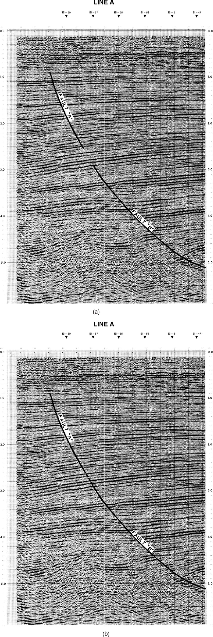
Figure 7-41 (a) The orientation of this seismic line is such that Faults A and B coincidentally line up and appear as if a one-fault trace could be drawn. (b) A one-fault interpretation forced through continuous reflectors (see dashed line). (From Tearpock and Harris 1987. Published by permission of Tenneco Oil Company.)
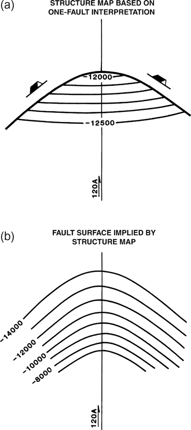
Figure 7-42 (a) Structure map of fault trap created by the forced interpretation. (b) Fault surface map generated from the one-fault interpretation (Fig. 7-41b). (From Tearpock and Harris 1987. Published by permission of Tenneco Oil Company.)
The concept of an implied fault surface map is described briefly in Chapter 8 and illustrated in Figure 8-54b; it is discussed in additional detail in Tearpock et al. 1994. It is tempting to create an implied fault surface from Figure 7-42a by connecting points of equal elevation along the fault trace with horizontal lines. Such a fault surface map, however, would imply that the fault is dipping toward the bottom of Figure 7-42a, whereas the seismic line in Figure 7-41 and the fault trace symbols on Figure 7-42a indicate the fault is dipping toward the top of Figure 7-42a.
The prospect was reviewed using the seismic line in Figure 7-41 and the additional lines in the surrounding area. First, based on the structure map in Figure 7-42a, the implied fault surface map in Figure 7-42b was prepared. Second, using all the available lines, the fault and structural interpretations in Figure 7-43a and b were made, which show two faults. The shallower fault is interpreted as a fault that is dying laterally away from an anticline to the west. It appears to die with depth on the seismic line (Fig. 7-41a), but actually the fault surface is simply migrating out of the plane of the line. The deeper fault is a buried growth fault that is also dying laterally, but in a generally opposite direction to that of the shallower fault. Seismic line 120A just happens to be in the correct orientation to make the two fault traces appear to line up on the profile. Figure 7-43 illustrates the correct fault surface and structural interpretation based on all the available data. Notice that based on this new and correct interpretation, there is no fault trap and therefore no prospect.
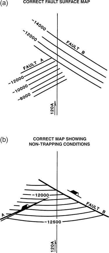
Figure 7-43 (a) Fault surface map for Faults A and B. (b) Completed structure map constructed by integration of fault and structure maps shows no hydrocarbon trap. (From Tearpock and Harris 1987. Published by permission of Tenneco Oil Company.)
The generation of this nonexistent prospect would not have occurred had the procedures outlined in this chapter been followed. First, a fault surface map should always be prepared. Had a fault surface map been prepared based on the one-fault interpretation and map, the sharp convex bend (in the downthrown direction) of the fault surface (Fig. 7-42b) should have been suspect and further review of the fault undertaken. Second, the construction of a vertical separation map would have shown a fault losing displacement with depth, then abruptly gaining displacement again, a very questionable and unlikely situation.
No prospect should be based on a single seismic line or even a few lines where more data are available. Too many illusions of geometry can occur on any given line. A gross underuse of costly 3D seismic data, frequently done to “save time,” is to use every fifth or tenth line to generate an interpretation and prospect. This means that only 10 to 20 percent of the seismic data are used. Companies spend millions of dollars to acquire and process 3D seismic surveys. The purpose is to provide a dense grid of data to improve the interpretation process. The use of every fifth or tenth line to generate an interpretation is at times a costly, unjustified shortcut that should not be accepted.
In Chapter 1, we stated that the only certainty in a subsurface interpretation, prepared from seismic and well log data, is that it is most likely incorrect. The best geoscientist is the one who comes up with the most accurate and geologically reasonable subsurface interpretation.
Remember the two significant causes of errors in geological interpretations and maps: the failure to use all the data available and the incorrect application of the data. If we fail to make fault surface and vertical separation maps, where the data are available, how can we expect our interpretation and resultant maps to be accurate, geologically reasonable, and representative of the best interpretation of the subsurface?
Growth Faults
One of the principal petroleum-related settings for normal faults is that of major large-scale gravity slide structures. The normal faults in this category decrease in dip with depth to low-angle faults, commonly becoming bedding-plane faults. These faults slide along a decollement and are called detachment faults (Chapter 11). Such fault systems are well known in areas such as the U.S. Gulf of Mexico, Brunei, and the Niger Delta. These faults are called listric growth normal faults, based on the Greek word listron, or shovel, because of their curved appearance in profile. The major listric fault on a structure is commonly referred to as the master fault if it has the largest relative displacement. Numerous synthetic and antithetic (secondary) faults are often associated with the master fault.
These listric growth faults are syndepositional, commonly exhibiting a significant increase in stratigraphic thickening in the downthrown (hanging wall) block and an increase in displacement with depth. This relationship indicates that there was movement along the fault surface while the sediments were being deposited (Chapter 13). Growth faults also are called syndepositional and contemporaneous faults because fault movement was occurring while the adjacent sediments were being deposited.
Growth faults are commonly associated with hanging wall anticlines, called rollovers, which develop as a result of the hanging wall block bending as it conforms to the curved fault surface (Suppe 1985) (see Chapter 10). These rollover anticlines are one of the most important hydrocarbon traps associated with listric growth faults.
Estimating the Vertical Separation for a Growth Fault
The method for estimating the missing section in a well due to a post-depositional fault, and thereby estimating vertical separation for the fault, was outlined in Chapter 4. In this section, we present two methods for estimating the vertical separation for a growth fault penetrated by a wellbore.
The Restored Top Method.
The thickness of the stratigraphic section in the footwall (upthrown) block of a growth fault is thinner than the equivalent stratigraphic section in the hanging wall (downthrown) block. Therefore, if a faulted well is correlated with a well in the upthrown block, the missing section due to the growth fault will be estimated to be smaller than if the correlation is made with a well in the downthrown block. So the procedure for estimating the vertical separation for a growth fault is not as straightforward as that for nongrowth faults. In most cases, at least two correlation well logs are needed: one located in the upthrown fault block and the other in the downthrown block. With the available electric well logs, the vertical separation at any horizon faulted out of a well can be estimated by the restored tops method, which is described in detail in Chapter 4.
Choose a horizon, faulted out of the subject well, for which you wish to estimate the vertical separation.
The log of a well in the upthrown block is then correlated with the deeper log section (the interval below the fault) in the faulted well in order to obtain an estimate of the upthrown restored top for the chosen horizon.
The log of a well in the downthrown block is correlated with the upper log section (the interval above the fault) in the faulted well in order to estimate the downthrown restored top for the horizon.
The estimate of vertical separation for the growth fault at the horizon is the difference in true vertical depths of the upthrown and downthrown restored tops for the horizon in the faulted well. If the wells are vertical, the difference in measured depths of the upthrown and downthrown restored tops can be used.
Using the cross section in Figure 7-44, we illustrate the use of the restored tops method. Fault 1 is a growth fault downthrown to the east. In Well No. 1, Beds A, B, and most of C are faulted out. Bed B is a horizon of interest to be mapped; therefore, we want to estimate the vertical separation for the growth fault at the level of Bed B. Three wells are on the cross section: Well No. 2 in the upthrown fault block, Well No. 3 in the downthrown fault block, and Well No. 1, which has the horizon of interest faulted out. If necessary, go back to Chapter 4 and review the section on estimating restored tops before continuing this section.
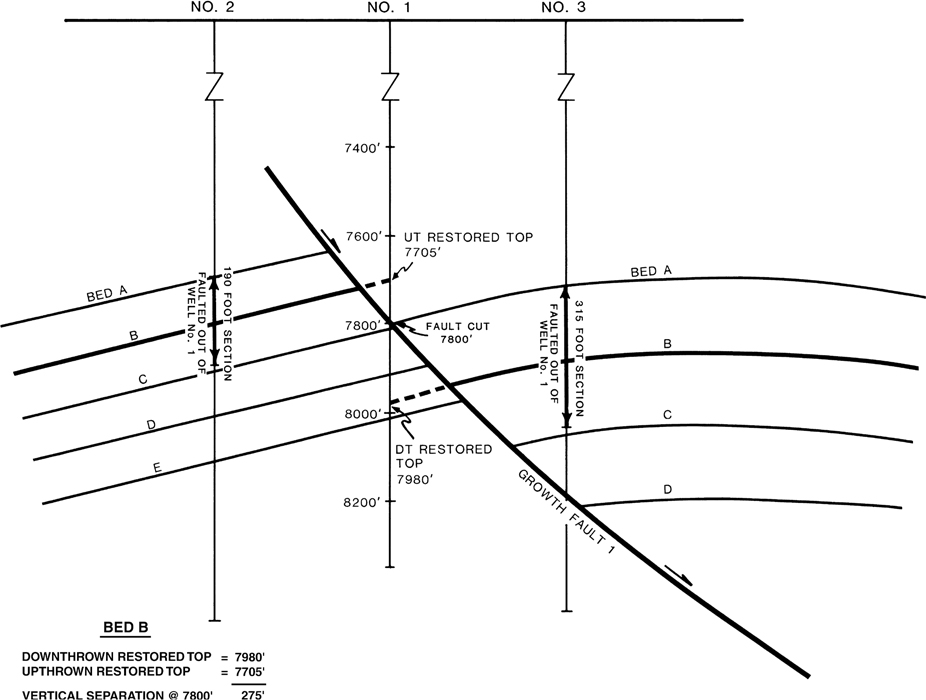
Figure 7-44 Cross section illustrates the restored tops method for estimating the vertical separation for a growth fault. The restored tops are estimates using the procedures discussed in Chapter 4.
First, estimate the missing section due to the fault in Well No. 1 using the other two wells (Fig. 7-44). By correlation with Well No. 2 in the upthrown fault block, the missing section at the fault in Well No 1 is 190 ft, but by correlation with Well No. 3 in the downthrown block, the missing section at the fault is 315 ft. Since these two estimates for the missing section are different, which one should be used as vertical separation in mapping Bed B? The answer is neither estimate. The 190-ft value is too small, since it is based on correlation with a well in the stratigraphically thin upthrown block. The 315-ft value is too large because it was obtained by correlation with a well in the stratigraphically thick downthrown block.
How do we obtain an estimate of the vertical separation for the growth fault to be used in the structure mapping of Bed B? The restored tops method outlined earlier must be used. The upthrown restored top for Bed B in Well No. 1, by correlation with Well No. 2 in the upthrown fault block, is at 7705 ft measured log depth (Fig. 7-44). The downthrown restored top in Well No. 1 for Bed B, by correlation with Well No. 3 in the downthrown Block, is at 7980 ft measured log depth. Using the restored tops method, the vertical separation for the growth fault at Bed B is estimated as the difference in restored top depths for Bed B (7980 ft − 7705 ft = 275 ft). Therefore, in the preparation of a structure map on Bed B, the vertical separation value of 275 ft is used to contour across Growth Fault 1. Also, in using this method, two additional control points for mapping are estimated, these being the upthrown and downthrown restored tops in Well No. 1. Remember, these tops must be corrected to true vertical subsea depths before they are used in the structure mapping of the horizon.
The estimated vertical separation of 275 ft for the fault cut for Bed B lies between the low value of 190 ft and the high value of 315 ft for missing section derived by correlation with wells on either side of the fault. The restored tops method is the most accepted procedure for estimating the vertical separation (missing section) on a growth fault at any particular horizon.
The Single-Well Method.
Given certain limitations, it is possible to use only one reference well to closely approximate the vertical separation for a growth fault. This method is referred to as the single-well method. It is applicable only if the given horizon is close to the top or to the base of the stratigraphic section missing in the faulted well. This method is illustrated in cross-sectional view in Figure 7-45.

Figure 7-45 The vertical separation is estimated for this growth fault using both the restored tops and single-well methods. The displacement is determined at the levels of Beds B, D, and F.
Three wells are in the cross section in Figure 7-45: Well No. 3 is in the upthrown fault block, Well No. 2 is in the downthrown fault block, and Well No. 5 is the well of interest. The growth fault has faulted out a significant stratigraphic section from Bed B through Bed F in Well No. 5. For mapping purposes, we are interested in the vertical separation for the growth fault at Beds B, D, and F.
First, we estimate the missing section in Well No. 5 with the other two wells (Fig. 7-45). By correlation with Well No. 3 in the upthrown block, the estimated missing section due to the growth fault is 200 ft, and with Well No. 2 in the expanded downthrown fault block, the estimated missing section is 400 ft. There is a two-to-one difference in the estimated missing section at the fault by correlation with these two wells. Which one is correct, or are they both correct? Which one, if any, should be used for vertical separation in the structure mapping of the various horizons? We know that this is a growth fault, which means by definition that the vertical separation increases with depth. Therefore, it is reasonable to assume that vertical separation increases from Bed B to Bed F. But by how much, and what is the vertical separation at each horizon?
The vertical separation at any horizon can be estimated by using the restored tops method, whereas the vertical separation at only two horizons can be estimated by using the single-well method. We begin by using restored tops to estimate the vertical separation at Bed B (Fig. 7-45). The upthrown restored top for Bed B is at 8050 ft, and the downthrown restored top is at 8250 ft. The difference between these two restored top values is 200 ft, which is an estimate of the vertical separation for the fault at Bed B. This is recorded within the inset in Figure 7-45, which contains a summary of the data pertinent to Beds B, D, and F.
The single-well method can be used to estimate the vertical separation for a growth fault, but it can be applied only under certain restraints. Notice in the cross section (Fig. 7-45) that Bed B is at the top of the section missing in Well No. 5; therefore, we can say that most of the interval faulted out of Well No. 5 can be represented by the thin upthrown section seen in Well No. 3. Therefore, the vertical separation at Bed B can be closely estimated simply by correlating Well No. 5 only with the thin upthrown Well No. 3. By making this correlation, we obtain an estimate of 200 ft for the missing section due to the fault. Observe the 200 ft of section faulted out of Well No. 5, as illustrated on the well log stick for Well No. 3. We can check the accuracy of this simplified technique by comparing the result with that obtained from the restored tops method (Fig. 7-45). They are the same. Using the two methods independently, the vertical separation of the growth fault at Bed B is estimated to be 200 ft.
Now estimate the vertical separation at Horizon F. First, using the restored tops method, the estimated vertical separation at this horizon is 400 ft. Again, the results are summarized in the insert in Figure 7-45. Reviewing the log sticks in cross section, notice that Bed F is at the base of the missing section in Well No. 5. Therefore, most of the section faulted out of Well No. 5 is represented by the thick downthrown section seen in Well No. 2. So, we can use the simplified single-well method and closely estimate the vertical separation at Bed F by correlating Well No. 5 with just one well, the thick downthrown Well No. 2. With this correlation, the vertical separation at Bed F is estimated to be 400 ft. Again, the estimate for the vertical separation is the same using the more detailed restored tops method or the simplified single-well method.
The last horizon requiring an estimated vertical separation is Bed D. Since Bed D is not near the top or bottom of the missing section in Well No. 5, the simplified single-well method cannot be used. Therefore, the restored tops method for estimating the vertical separation at Bed D must be used, and it is illustrated in Figure 7-45. The upthrown restored top is at 8150 ft, and the downthrown restored top is at 8450 ft, resulting in an estimated vertical separation of 300 ft at Bed D.
Figure 7-46 shows a portion of the structure map for each of the three horizons, Beds B, D, and F. For mapping purposes, well depths are converted to subsea depths by using a KB = 50 ft for each well. The beds are dipping, and their apparent dip is horizontal in the cross section in Figure 7-45. The maps were accurately constructed by the integration of the growth-fault surface map with each horizon map, as described in Chapter 8. Note how the restored tops for Well No. 5 are honored by the structure contours. The maps collectively demonstrate that the fault gap widens with the increase in vertical separation with depth, as is typical for any growth fault delineated on a set of horizon maps. Also, from map to map, the position of Well No. 5, within the fault gap, changes relative to the upthrown and downthrown traces of the fault. That also is typical for any well in which mapped horizons are faulted out by the same fault. Compare the three maps with the cross section in Figure 7-45 to visualize why the position of Well No. 5 changes relative to the traces of the fault. If the horizon being mapped is at or near the top of the missing section in the faulted well, the fault size vertical separation can be closely approximated by using the single-well method and correlating the faulted well with a nearby well in the thin upthrown fault block. See Bed B in our example in Figure 7-44. In map view, this is represented in Figure 7-45a, which is a portion of the structure map on Bed B.
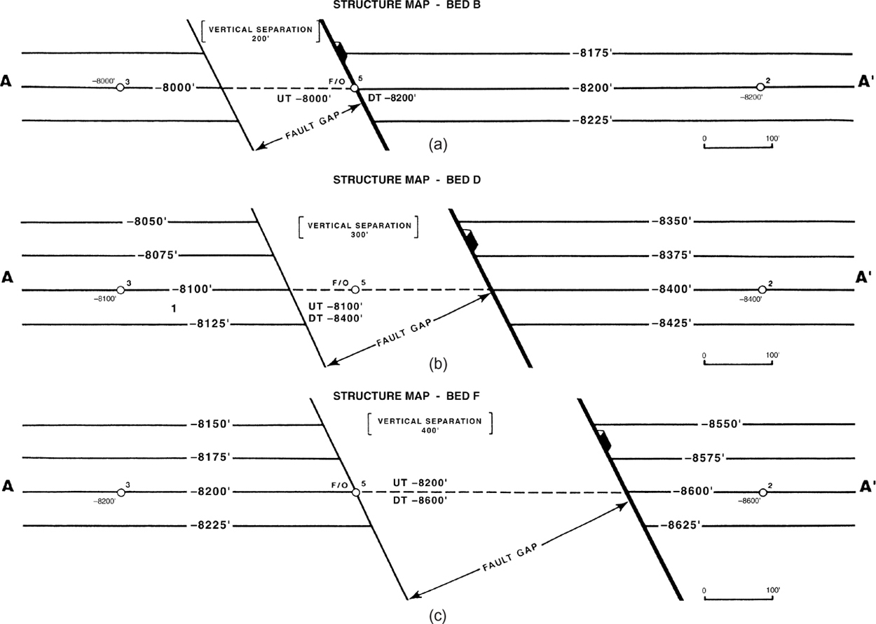
Figure 7-46 Segments of the integrated structure maps for Beds B, D, and F. Notice how the fault gap width changes with depth in response to the increase in vertical separation. Well depths are converted to subsea depths (KB = 50 ft for each well).
If the horizon being mapped is at or near the bottom of the missing section in the faulted well, the missing section fault size can be closely approximated by using the single-well method and correlating the faulted well with a nearby well in the thick downthrown fault block. This was done for Bed F, as shown in Figure 7-46. In map view, this is represented in Figure 7-47c, which is a portion of the structure map on Bed F. The faulted Well No. 5 is near the upthrown trace of the growth fault. If the horizon being mapped falls clearly within the missing section in the well log (D Horizon, Fig. 7-44), then the restored tops method must be used. The restored tops method is always preferable over the single-well method if time is not a factor. In addition to providing an estimate of vertical separation for the fault at any horizon, it also contributes two control points for contouring (the upthrown and downthrown restored tops).

Figure 7-47 (a) Fault surface map of a growth fault. Vertical separation contours are placed on the fault map, adding valuable mapping information pertaining to the growth fault. (b) Vertical separation values are not contoured, but strategically placed on the fault surface map, which is a shortcut method. (From Tearpock and Harris 1987. Published by permission of Tenneco Oil Company.)
The faults used to illustrate the methods for estimating the vertical separation for a growth fault do possess linear expansion, and the beds are gently dipping in Figure 7-46. However, these methods are just as applicable for growth faults with nonlinear expansion and in areas with steeply dipping beds.
Growth-Fault Surface Map Construction
Earlier in the chapter, we discussed the importance of preparing a fault surface map for all faults. The procedures and guidelines for constructing fault surface maps as outlined earlier are applicable to growth faults, with one possible addition. Recall we stated that a good geological mapping practice is to contour the vertical separation for the fault, as well as the fault surface (Fig. 7-40a). With a growth fault, however, it is absolutely necessary to contour both the fault surface and vertical separation, whenever possible. The vertical separation for a growth fault varies with depth and changes laterally, and in some cases rather abruptly. Therefore, in order to prepare an accurate interpretation of the fault for future mapping and prospecting, both the fault surface and vertical separation should be mapped.
The vertical separation data for a fault can come from electric well logs or seismic sections. Once the vertical separation data are gathered, there are at least two ways to map the data. The vertical separation values can be contoured on the fault surface map as shown in Figure 7-47a, or they can be recorded at strategic locations on the fault surface map as shown in Figure 7-47b. The actual contouring of the vertical separation is by far the more accurate method and the one we recommend.
Looking at the fault surface and vertical separation contour map in Figure 7-47a (which is only a segment of the entire fault), we can quickly observe a lot of valuable information about this growth fault. The sources of the fault surface and vertical separation data are both well logs and seismic sections. The fault surface contour spacing indicates that the fault has a listric shape with a maximum dip rate of 60 deg at around −5000 ft, decreasing to 40 deg at about −11,000 ft. Both the vertical separation values next to each well and seismic shotpoint and the vertical separation contours indicate that the vertical separation increases with depth from 250 ft at −4688 ft in Well No. 12 to 590 ft at −10,847 ft in Well No. 3. Based on the spacing of the vertical separation contours, the fault growth appears to be generally uniform over this area of the fault. Also, the contours show that the vertical separation increases laterally from the northeast to the southwest. Taking the −9000 fault contour as an example, in the southernmost portion of the map, the vertical separation at this depth is 500 ft. Following along this −9000-ft contour to the northeast, this displacement decreases steadily to only 400 ft at the northern end of the map. Lastly, the contours point to the direction of maximum growth fault activity (major sedimentary depocenter for this fault) as being to the southwest. All this information is important for future integration of this fault interpretation with structure and stratigraphic data to prepare detailed structure and isochore maps for use in the exploration and exploitation of localized hydrocarbon accumulations.
The pattern of fault surface and vertical separation contours is different for nongrowth (structural) faults than it is for growth faults. Refer once again to Figure 7-40a and the discussion. Compare this map with that for the growth fault in Figure 7-47a. Identify the differences observed and establish criteria that can be used to distinguish a growth fault from a post-depositional fault using the fault maps.
Directional Surveys and Fault Surface Maps
In Chapter 3 we discuss the importance of using the directional survey from a deviated well to calculate the position and depth of the borehole throughout its entire length. Recall that we illustrate the two basic ways in which directional well paths are presented on a map base, shown here again as Figure 7-48a and b.
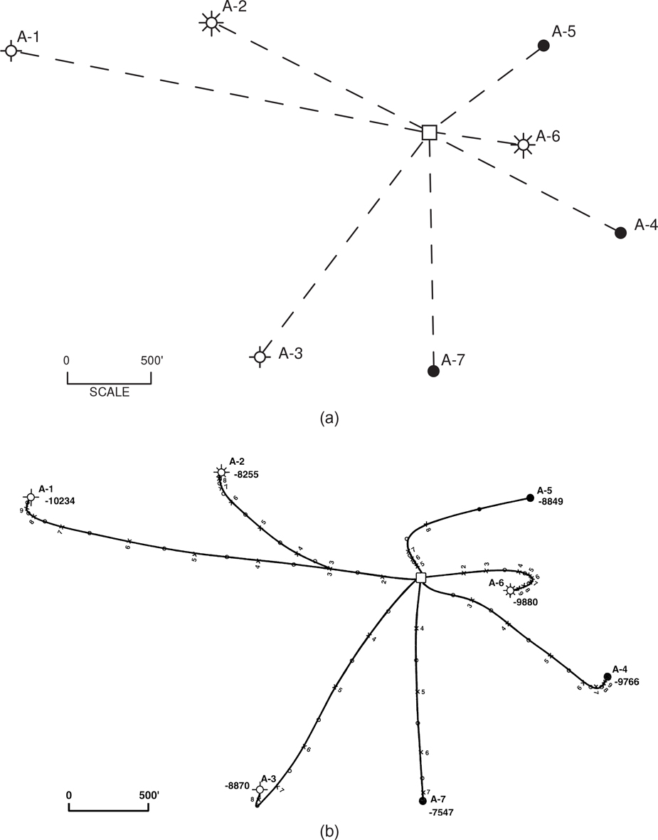
Figure 7-48 (a) Straight-line method of plotting directional wells in map view. (b) Detailed plot of directional survey data indicating the location and subsea depth of each wellbore along its entire length.
Using the simplified method of plotting a directional well shown in Figure 7-48a, the only data required and plotted on the basemap are the surface and bottomhole locations. At times the measured depth to total depth may be recorded next to the bottomhole location. Between the surface and bottomhole locations, a straight dashed line is usually drawn. This directional well plot provides absolutely no information about the position or depth of the wellbore in the subsurface between the surface and bottomhole locations. Such a plot is not helpful in the interpretation, construction, and evaluation of fault, structure, or isochore maps.
Where directional survey data are actually plotted to provide detail regarding the position and subsea depth of the wellbore throughout its entire length, as shown in Figure 7-48b, the plot has real value. Such a plot provides a visual guide (in map view) to the location and subsea depth of the wellbore anywhere along its path. Such a plot saves time in preparing subsurface maps and is extremely helpful in the interpretation, construction, and evaluation of fault, structure, and isochore maps. In this section, we look at several important benefits of fault surface mapping derived from plotting the actual position and subsea depth, at evenly spaced increments (usually 500 ft or 1000 ft), of all directional wells on a basemap. The benefits to structure and isochore mapping are covered in the appropriate chapters.
The advent of computer mapping systems has rendered the issue of basemaps largely moot, as computers have no problem in correctly plotting fault cuts and horizon picks in their proper X-Y location. Some database programs, such as Lexco’s OWL for the Gulf of Mexico, still use the simplified method illustrated in Figure 7-48a because of the speed of mapping. All software mapping programs with which we are familiar use the more accurate method illustrated in Figure 7-48b. Tearpock and Bischke (1991, 2003) discussed the relative merits of the two methods in some detail, and interested readers are referred to these references.
Directional Well Pitfalls
When is a straight hole not a straight hole? When it is deviated. Many so-called vertical wells are not vertical at all but have been drilled at a deviated angle, as discussed in Chapter 3. This deviation usually is not planned but is the result of natural wellbore drift. As we discuss in Chapter 3, the deviation angle of a drilling well may be monitored in some way, such as with a Totco survey. Remember that a Totco records the deviation angle of the well but not its direction. Most countries have regulations allowing a maximum deviation before an actual directional survey is required by law. Not all wells that are designed to be vertical, however, are monitored for deviation.
The fault surface maps in Figure 7-49a and b illustrate the kinds of problems that can arise when wells are assumed to be vertical or when no directional well data are available. The fault surface map in Figure 7-49a was prepared using the available well data shown on the map. Each depth value represents the subsea depth at which this mapped fault was encountered in the adjacent well. The map does not look too bad, but it does have some unusual variations in contour spacing (dip of fault) and indicates a problem in the northeast part of the map. According to the available data on the basemap and electric logs, all the wells are identified as being vertical. However, looking at the fault surface map, it is apparent that something is wrong. Either the fault picks are incorrect, the wells are spotted at the wrong surface location, or some of these vertical wells are not vertical.
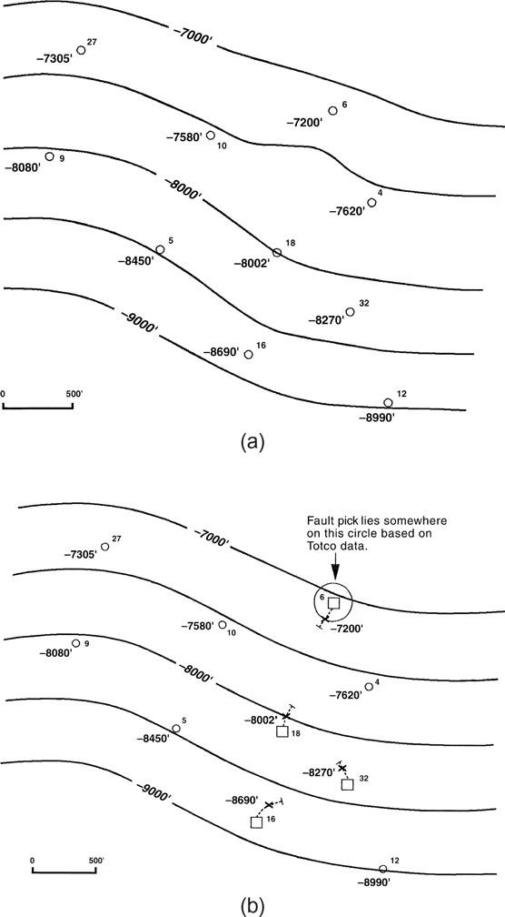
Figure 7-49 (a) Fault surface map prepared with the assumption that all the wells are vertical. Notice the unrealistic variations in dip in the northeast portion of the map. (b) Revised fault surface map based on new directional well data obtained for a number of wells. The new interpretation of the fault surface appears reasonable.
The answer to the problem is shown in Figure 7-49b. Upon additional review of well files, five wells were found to be deviated, as shown in the figure. By replotting the wellbores as deviated wells and respotting the fault picks to correspond to the true wellbore deviation, the fault surface map shown in this figure was constructed.
Well No. 6 is of special interest. The only available directional data on this well was a Totco survey, which measures angle but not direction. In the case of Well No. 6, the assumption was made that the deviation was all in the same direction. Therefore, a circle whose radius is equal to the distance the well could have deviated from the vertical to a depth of −7200 ft was plotted. If the wellbore deviation were all in the same direction, the fault pick should fall somewhere on this circle. The direction of deviation that best fit the fault was used to spot the pick, as shown in the figure. Notice that the contour spacing has evened out and the major contouring problem in the northeast was resolved.
Keep this example in mind, especially when mapping in areas with very old wells. A problem that might at first appear to be that of wrong correlations or an incorrect interpretation might turn out to be nothing more than a problem of a vertical well not being vertical. If the issue is important and the wellbore is still available, it is worthwhile to re-enter the well and run a new, modern directional survey.
Fault Maps, Directional Wells, and Repeated Sections
In Chapter 4 we discuss the specific geometry between a normal fault and a directional well required for a repeated section (Fig. 4-36). We also look at several examples of repeated sections, such as the one in the Texaco LL&E Well No. 212 (Fig. 4-38).
In the preparation of a fault surface map, a fault resulting in a repeated section is treated in the same manner as a fault resulting in a missing section. Figure 7-50 shows the Texaco LL&E Well No. 212 plotted in cross section along the wellbore deviation path. The well/fault geometry is quite unique in that the well crosses the same Fault H at least four times: twice in the normal sense, resulting in missing section, and twice in the reverse sense, causing two repeated sections. Therefore, the well actually penetrates the downthrown fault block three times and the upthrown block twice.
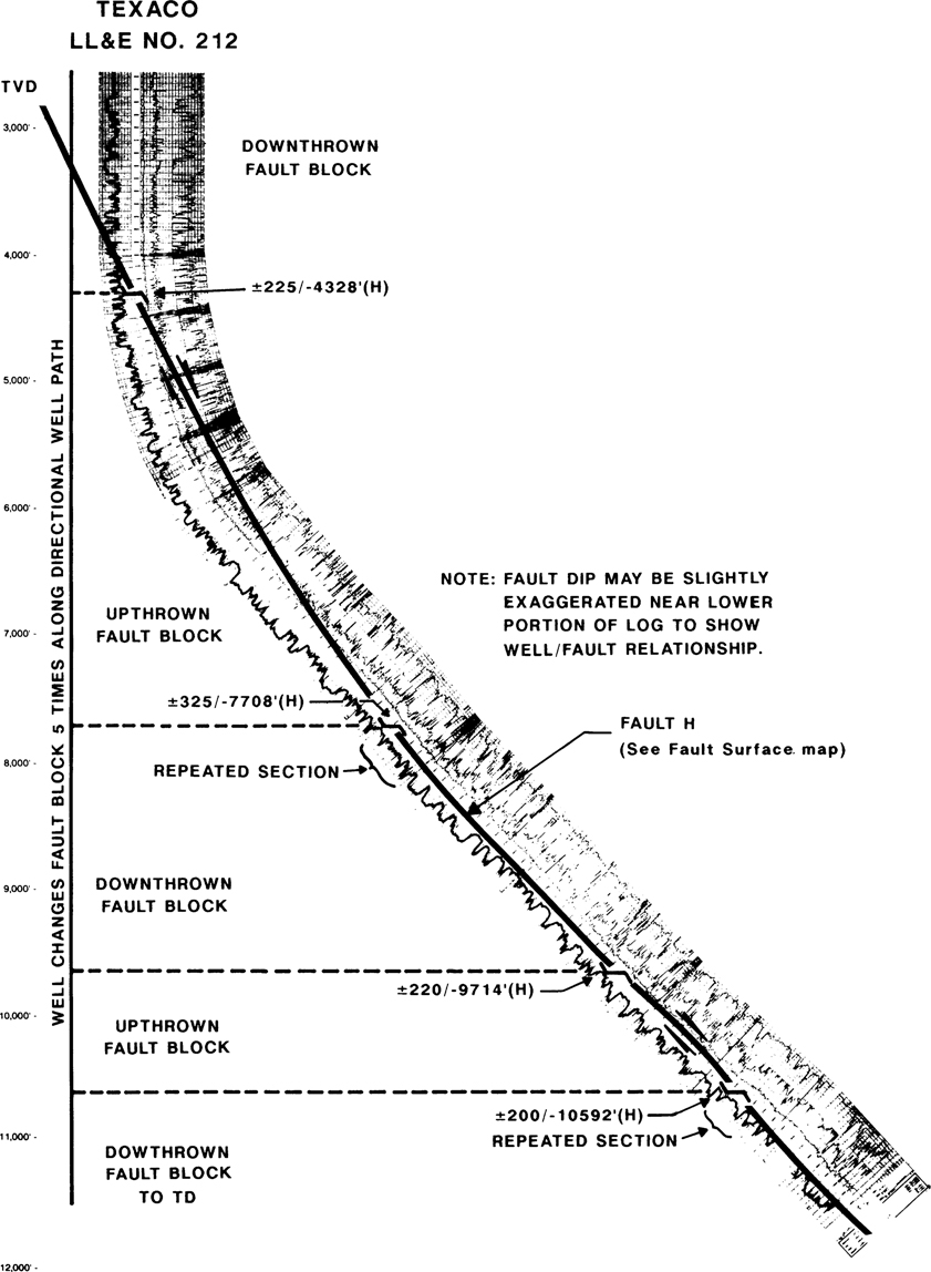
Figure 7-50 Directionally drilled Well No. 212 intersects Fault H four times, resulting in two missing sections and two repeated sections. The well changes fault blocks four times. (Published by permission of Texaco, USA.)
Figure 7-51 shows a portion of the fault surface map for Fault H, in the vicinity of Well No. 212. The four fault picks in the well and fault control data from numerous straight holes and other deviated wells were used to prepare the fault surface interpretation shown. The fault surface has a generally listric shape but displays little if any growth. Near the total depth of the well, Fault H intersects and terminates against Fault C, which is a down-to-the-north fault. Faults E, E-1, and B-1 are interpreted as terminating against Fault H, as shown in Figure 7-51. These faults are not shown in the cross section in Figure 7-50. This example shows the unusual geometries that can occur where directional wells encounter fault surfaces.
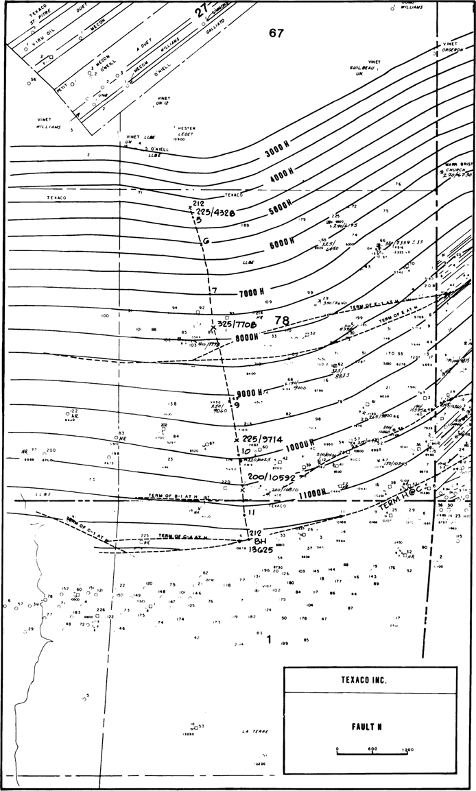
Figure 7-51 Portion of the fault map for Fault H. Note the four fault data points from Well No. 212. (Published by permission of Texaco, USA.)
Vertical Separation—Correction Factor and Documentation
The vertical separation for a nongrowth fault, as discussed in Chapter 4, is equal to the vertical thickness of the missing or repeated section in a well. In vertical wells the thickness represented on a log is the true vertical thickness. Therefore, when correlating a fault in a well log with another log from a vertical well, the vertical separation for the fault is the measured amount of missing or repeated stratigraphic section determined from the vertical well log.
For directionally drilled wells, the log thickness can be greater or less than true vertical thickness. Therefore, a correction must be applied to the log thickness to obtain its true vertical equivalent. The equations used for this conversion are presented in Chapter 4.
The vertical separation for a growth fault penetrated by a well should be determined at specific horizons by using the difference in restored tops for each horizon faulted out of the well. Where a deviated well is the reference well for determining the interval thicknesses to be used to restore tops, each thickness must be converted to true vertical thickness.
As discussed in Chapter 1, good-quality work must be backed up by good documentation. This means recording all the data in some format that can be easily used or revised by the person conducting the work, supervisors or managers, other team members, or persons inheriting an area for future study. Fault data must be documented, particularly when deviated wells are used for correlation and require correction factors for log thickness in order to determine the correct value for missing or repeated section. This need for documentation is irrespective of whether correlating and mapping is being done by hand or on a computer workstation. If being done on a workstation, fault data must be documented in the computer database if the software allows it, as most interpretation packages do. If the interpretation software being used does not allow recording the fault data, this data must be recorded separately where it is easily accessible to other workers.