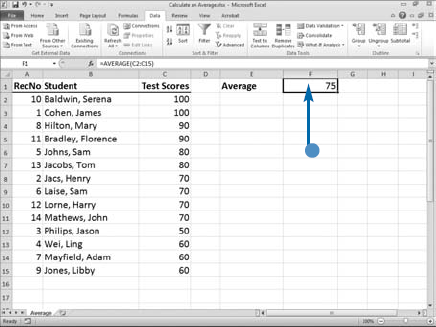
An average is the sum of two or more values divided by the total number of values. You can use the AVERAGE function to calculate an average. The AVERAGE function takes one type of argument: Number1 through Number255. An array is a list of values enclosed in curly braces. For example {20, 25, 25, 30} is an array. In each Number argument, you can enter a number, a range that contains numbers, a range name, or an array. The AVERAGE function sums each value you enter and divides by the total number of values. If a cell contains a zero, Excel includes the value in the calculation. If a cell is blank, Excel does not include the cell in the calculation.

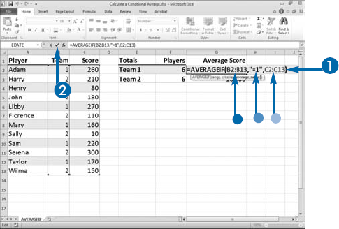
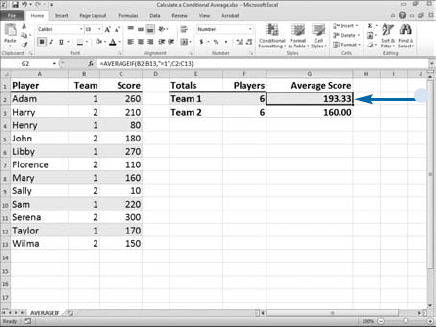
The AVERAGEIF function combines the AVERAGE function with the IF function. You can use the AVERAGEIF function to compute an average for data that meets the criteria you specify. For example, you can create a function that evaluates a list to determine the team a person is on, and then averages the scores of all the people on Team 1.
AVERAGEIF takes three arguments: Range, the range of values you want to evaluate by using the criteria you specify in the Criteria argument; Criteria, the criteria you want to apply to the range; and Average_range, the range of cells you want to average. The third argument, Average_range, is optional. If you do not include it, Excel averages the range you specify in the Range argument.
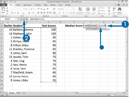
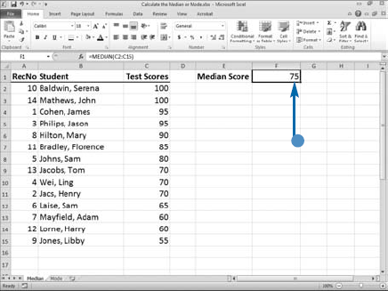
When analyzing data, you may need to find the median. The median is the midpoint in a series of numbers, the point at which half the values are greater than the others and half the values are less than the others when you arrange the values in numerical order. If you are analyzing the scores students receive on a test and the median score is 75, half the students received a score greater than 75 and half the students received a score less than 75. When finding the median, if the number of items in the series is even, the median is the average of the two middle values. For example, in the series 100, 95, 90, 80, 60, 50, 40, the median is the number 80 because three numbers are greater than 80 and three numbers are less than 80. In the series 100, 95, 90, 80, 70, 60, 50, 40, the median is 75 — the average of 80 and 70. You can use Excel's MEDIAN function to calculate the median.
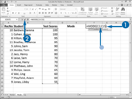
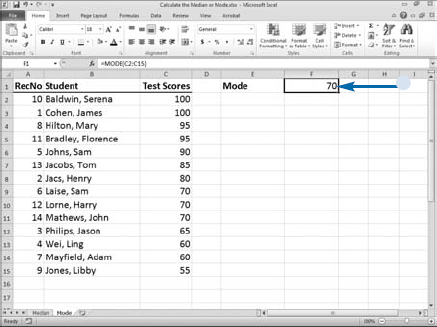
The mode is the most common value in a list of values. For example, if your list of values is 70, 65, 90, 70, 70, 90, 60, the mode is 70 because it is the value that occurs most often. You can use Excel's MODE function to find the mode.
Both the MEDIAN and MODE functions take one type of argument, Number1 through Number255. An array is a list of values enclosed in curly braces. For example {20, 25, 25, 30} is an array. In each Number argument, you can enter a number, a range that contains numbers, a range name, or an array.
Sometimes you want to find how one thing ranks in relation to other thing. For example, you might want to find out how a particular student's test score ranks in relation to all other students: Did the student receive the highest score, the second highest score, and so on? The RANK.EQ function ranks a number relative to other numbers in a list. If you sort a list in numerical order, the rank is equal to the position where the number would fall in the list. You can tell the RANK.EQ function whether the list you want to base the rank on should be sorted in ascending order or descending order.
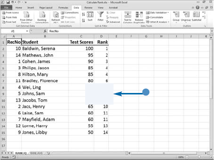
If two numbers have the same value, the RANK.EQ function gives them the same rank. For example, in the list 100, 95, 90, 85, 85, 80, 70, the RANK.EQ function ranks the number 85 fourth. If two or more numbers have the same rank, subsequent numbers are affected. In the preceding list, the RANK.EQ function ranks 80 sixth.
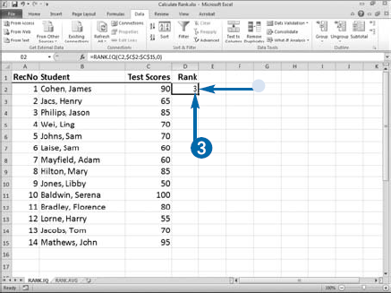
The RANK.EQ function takes three arguments: Number, the number for which you want to find the rank in a list; Ref, the array or cell range with the list; and Order, the order in which you want to sort the list. Type a 0 or omit the Order argument if you want to sort the list in descending order. Type a nonzero value if you want to sort the list in ascending order. When using the RANK.EQ function, if you reference nonnumeric values, the RANK.EQ function ignores them.
Calculate Rank

The number you want to rank.
The array or range you want to evaluate.
The list order. Enter 0 for descending or 1 for ascending.

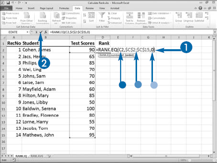
Excel ranks the number.

Note: See Chapter 12 to learn how to use the fill handle.

Note: See Chapter 8 to learn how to sort a list.
If two or more numbers are the same, Excel gives them the same rank.
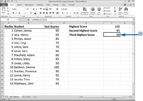
Sometimes you want to identify the top values in a series. For example, you might want to find the highest, second highest, and third highest score on a test.
The LARGE function evaluates a series of numbers and determines the highest value, second highest, or Nth highest value in the series, with N being a value's rank order. LARGE takes two arguments: Array, the array or range of cells you want to evaluate, and K, the rank order of the value you are seeking, with 1 being the highest, 2 the next highest, and so on. The result of the LARGE function is the value you requested.
Another way to determine the first, second, or Nth number in a series is to sort the numbers from largest to smallest and then simply read the results. See Chapter 8 to learn how to sort. This technique is less useful when you have a long list or when you want to use the result in another function.
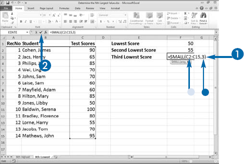
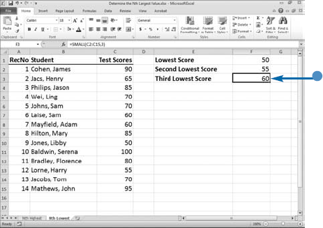
Another useful function that works in a fashion similar to the LARGE function is the SMALL function. The SMALL function evaluates a range of values and returns the smallest value, second smallest, or Nth smallest in a series. SMALL also takes two arguments: Array, the range of cells you want to evaluate, and K, the rank order of the value you are seeking, with 1 being the lowest, 2 the next lowest, and so on. For example, if you enter 1 as the K value, it returns the lowest number; if you enter 2, it returns the next lowest, and so on.
Determine the Nth Largest Value
Calculate the Nth Highest Value
The array or range you want to evaluate.
The rank order you want to find.
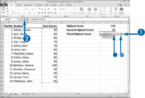
Excel calculates the results.
Calculate the Nth Lowest Value
The array or range you want to evaluate.
The rank order you want to find.
Excel calculates the results.
Extra
To better describe the function, Excel 2010 renamed the PERCENTRANK function PERCENTRANK.INC. For backwards compatibility, the PERCENTRANK function is still available.
You can use the PERCENTRANK.INC function to determine the rank of a value as a percentage of all the values in your data set. The PERCENTRANK.INC function takes three arguments: Array, the array or range you want to use to determine the percent rank; X, the value you want to rank; and Significance, the number of significant digits you want your results to return. The default is three digits. If you leave this argument blank, the PERCENTRANK.INC function uses the default.
The PERCENTRANK.INC function gives equal values the same rank. If you want to format the value returned as a percentage, select the cell, click the Home tab, and then click the Percent Style button (
Excel 2010 added PERCENTRANK.EXC to comply with industry standards for calculating the rank of a value as a percentage of all the values in a data set. The PERCENTRANK.EXC takes the same arguments as PERCENTRANK.INC. It excludes the ranks of 0 and 100.
When you collect large amounts of data, organizing your data can help you see patterns. Usually, you start by sorting your data so you can see the range of values. The next step might be to do a simple frequency distribution so you can see how often each value occurs. To understand your data further, you might create a grouped frequency distribution. Grouping your data makes it easy for you to compare categories of data.
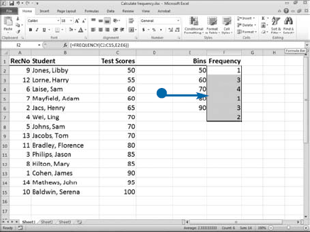
You can use Excel's FREQUENCY function to group your data into categories. For example, you can use the FREQUENCY function to display student test scores. The first group might be scores less than or equal to 50, representing scores 50 percent or lower; your second group might be 51 to 60; the next group 61 to 70, and so on, up to scores of 90 percent or higher. Excel counts the number of occurrences in each group.
You must supply the FREQUENCY function with two arguments: the Data_array and the Bins_array. The Data_array is the list of values you want to group. The Bins_array is the list of groupings you want to use. To use the FREQUENCY function, you must select the cells into which you want to place your results. If you have five groups, select six cells — one more cell than the number of groups you have. Type the function or enter it into the Function Arguments dialog box. Frequency is an array function; curly braces must surround your function. Press Ctrl+Shift+Enter after you enter your arguments. Excel will place curly braces around your function. If curly braces do not surround your function, your function will not calculate.


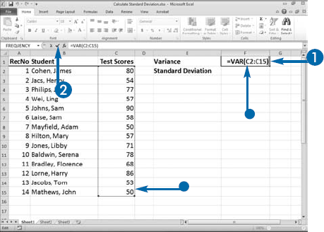
Statisticians refer to the average of a group of values as the mean. When you have a list of numbers, you can use the variance and standard deviation to show how much a group of numbers varies from the mean — the larger the variance, the more the values vary.
When manually calculating variance, you start by calculating the mean of all the values in your list, and then you subtract each value in the list from the mean value. This tells you how much each value deviates from the mean. You then square each deviation, sum the squared deviations, and then divide the sum by the number of values minus 1 to obtain the variance.
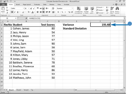
Instead of performing this complex calculation to calculate the variance, you can use the VAR function to obtain the variance. The VAR function takes one type of argument, Number1 through Number255. An array is a list of values enclosed in curly braces. For example {20, 25, 25, 30} is an array. In each Number argument, you can enter a number, a range that contains numbers, a range name, or an array.
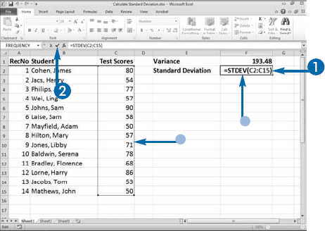
Finding the variance is often useful, but because the variance is a squared value, it is difficult to interpret the variance in relation to the mean. Therefore, statisticians often calculate the square root of the variance. They call the resulting value the standard deviation. You can use Excel's STDEV function to calculate the standard deviation. The STDEV function takes the same type of argument as the VAR function and works in much the same way.

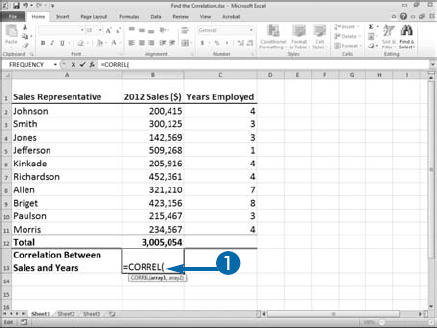
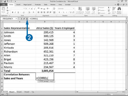
With the CORREL function, you can measure the relationship between two variables. You can explore questions such as whether there is a correlation between years employed and sales. A correlation does not prove one thing causes another. The most you can say is that one number varies with the other. Their variation may be the result of how you measured your numbers or the result of some factor underlying both variables. When you use correlations, you start with a theory that two things are related. If there is a correlation, you must then gather evidence and develop plausible reasons for the correlation.
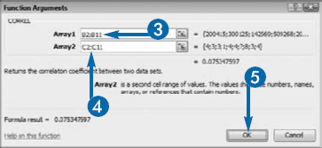
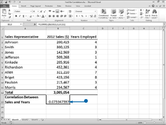
Use the CORREL function to determine a correlation. CORREL takes two arguments: array1 and array2 — the two lists of numbers. The result of the function is a number, r, between −1 and 1. The closer r gets to −1 or 1, the stronger the relationship. If r is close to or equal to 0, that means that there is little to no correlation between the variables. If r is negative, the relationship is an inverse relationship — for example, as years employed increases, sales decrease. A positive result suggests that as one variable increases, so does the other. For example, as years employed increases, sales increase.
When using CORREL, if a reference cell contains text, logical values, or empty cells, Excel ignores those values. However, reference cells that contain a value of 0 are included in the calculation. If the number of data points in array1 and array2 are not equal, Excel returns the error message #N/A.
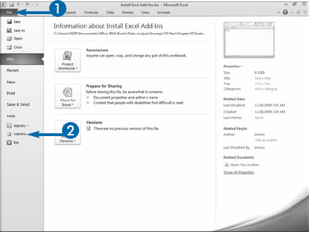
Installing add-ins gives you additional Excel features not available in the Ribbon by default. An add-in is software that adds one or more features to Excel. Bundled add-in software is included with Excel but is not automatically installed when you install Excel. There are several add-ins that come standard with Excel, including Solver, which enables you to solve optimization problems easily; the Euro Currency Tools, which enable you to calculate exchange rates between the Euro and other currencies; and the Data Analysis Toolpak, which provides you with a number of tools you can use for statistical analysis. The remainder of this chapter introduces a few of the statistical add-ins in the Data Analysis Toolpak.
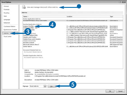
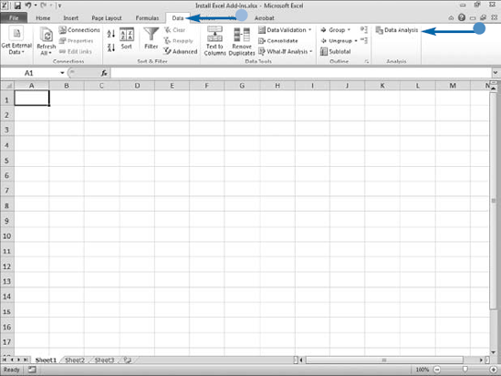
You install the bundled add-ins by using the Excel Options dialog box. You can find them in the Add-Ins section. Once installed, add-ins are available right away. They usually appear on a tab related to their function. The Data Analysis Toolpak appears on the Data tab.
You can also take advantage of third-party add-ins to gain functionality in support of advanced work in chemistry, risk analysis, modeling, project management, statistics, and other fields. Third-party add-ins usually have their own installation and usage procedures. Consult the vendors of these programs for documentation.
To learn about special-purpose Excel add-ins in your field, you can perform a Google search by going to www.google.com. Your search terms should include Excel, the field of knowledge — for example, chemistry — and other relevant information, such as a vendor's name. Third-party vendors are responsible for supporting their own products.

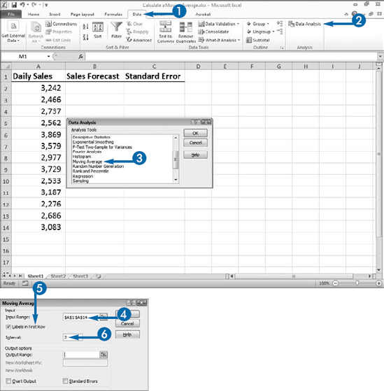
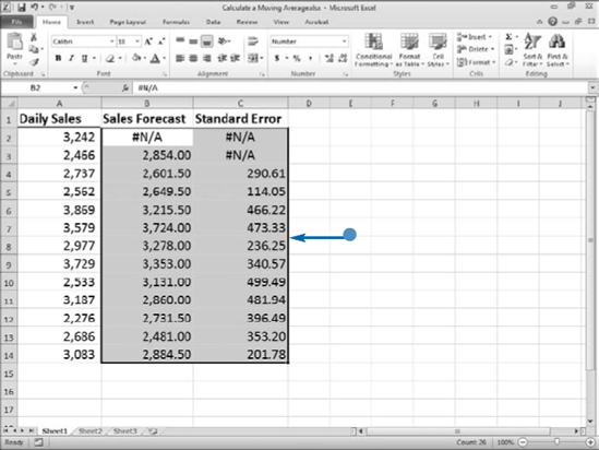
The Moving Average tool projects values based on the average value over a specified period. Using a moving average can reveal trends that are masked when you use a simple average because a simple average gives equal weight to each value. A moving average weighs recent values equally and ignores older values, thereby enabling you to spot trends. You can use a moving average to forecast sales, stock prices, or other trends.
You specify the number of values, or intervals, Excel should use to calculate the moving average. If you do not supply an interval, Excel uses the default value of 3, which means that the moving average is calculated by averaging the last three values.
Unlike other tools available for Data Analysis, the Moving Average tool can only output the values to the current worksheet. You need to specify the first cell you want to use for the results. If the first row contains a label, your data should start in the second row. In addition to a forecast, you can elect to have Excel compute the standard error. If you select this option, Excel creates an additional column that contains the standard error.
You can also create a chart that shows the relationship between the actual values in the data set and the forecasted moving average. If you select this option, Excel places the chart on the same worksheet as the moving average values.
Excel provides the Moving Average tool as part of the Data Analysis Toolpak. See the previous section, "Install Excel Add-Ins," to learn how to install the Data Analysis Toolpak.

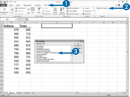
You can use an F-test to determine whether two variances are equal. Variance is a measurement of how much a group of values varies from the group's mean value. For example, if you have two plants producing the same product, one in Indiana and one in Texas, and both have efficiency levels of 95 percent, but you want to know which plant remained consistently more efficient throughout the year; you can perform an F-test. If you find that the Indiana plant has a lower variance than the Texas plant, you know that the Indiana plant was consistently more efficient.
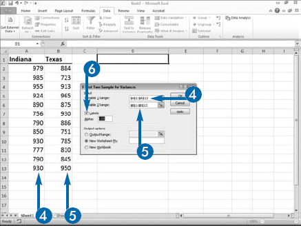
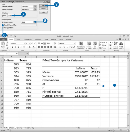
When you use an F-test analysis, Excel compares the ratio of the variance between the two groups of data. Excel calculates an F statistic (F) for the two sets of data, which is the ratio of the Mean Standard Square Error (MS) between the groups to the MS within the groups. If the F statistic is less than the F critical value, you cannot reject the null hypothesis that the variances of the two groups are the same. An F statistic close to 1 indicates that two groups have equal variances.
To perform this test, you must provide Excel with the ranges of both data groups as well as an Alpha level, or the statistical confidence level you expect. The Alpha field is the probability of the null hypothesis being true. You specify a value between 0 and 1 for the confidence level. The default level of .05 is equivalent to a 95 percent confidence level. To make your table easily identifiable, you can let Excel know that you have labels in the first row of your worksheet.
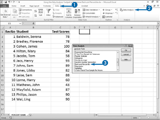
If you want to rank a series of values in a list, you can use the Rank and Percentile tool. With this tool, Excel takes a list of numeric values and ranks them from highest to lowest by both a numeric and a percentage value. It also calculates a percentile for your value. For example, you may want to rank the test scores of the students in a class to show not only which person had the highest score but also to determine the student's percentile when compared to the entire class. This feature is perfect for ranking the top-selling item, the most efficient facility within a company, or the machine or team that produces the highest level of output.
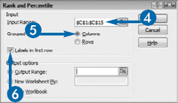
You can only rank one row or column of values at a time. Excel enables you to select multiple rows or columns as the input range, but only analyzes the first row or column. You can only have a label in the first row of a column. If the specified range contains any other text, an error message displays.
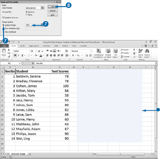
You can output the results of the Rank and Percentile tool to a specific range of cells within the current worksheet, a new worksheet, or a new workbook. If you select New Worksheet, you can specify the worksheet name or allow Excel to assign a default name.
Excel provides the Rank and Percentile tool as part of the Data Analysis Toolpak. See the section "Install Excel Add-Ins" to learn how to install the Data Analysis Toolpak.
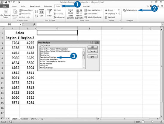
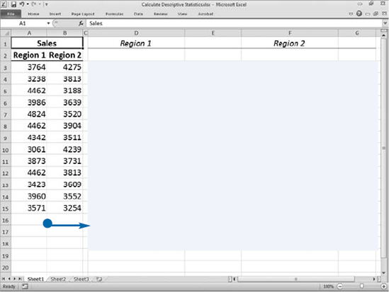
You can have Excel quickly calculate 16 different statistical measurements and summarize them in a list using the Descriptive Statistics tool. For an analyst, this feature is perfect for calculating statistical information on large databases or worksheets. When you use this tool, Excel produces a table containing standard statistical calculations for each group of data values in your list, including the mean, standard error, median, mode, standard deviation, sample variance, kurtosis, skewness, range, minimum, maximum, sum, count, largest value, smallest value, and confidence level. For example, if you use it to compare a list containing sales amounts for different regions, Excel produces a table containing the statistical values related to each region.
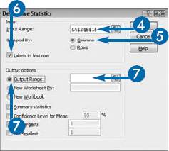
With the Descriptive Statistics tool, you must specify the range of cells containing the sets of data. You also must indicate whether you have your data sets grouped in rows or in columns. Each row or column must contain a different set of data. You can make the output easier to identify by labeling your data.
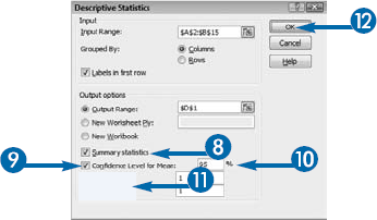
You can use the last four options in the Descriptive Statistics dialog box to specify which descriptive statistic values Excel calculates. Use the Summary Statistics option to calculate all the common descriptive statistic values. Use the Confidence Level for Mean option to calculate the confidence level. Kth Largest and Kth Smallest enable you to find specific values in the group, such as the second smallest or third largest number. If you specify a value of 1, you receive the same values Excel gives you for the minimum and maximum values.