
When processing a sound recording, sound engineers often face the need to apply specific digital audio effects to certain sounds only. For instance, the remastering of a music recording may require the correction of the tuning of a mistuned instrument or the relocation of that instrument in space without affecting the sound of other instruments. This operation is straightforward when these sounds are available as separate tracks, but becomes quite difficult otherwise. Indeed, the digital audio effects reviewed in this book all apply to the recording as a whole.
Source separation refers to the range of techniques aiming to extract the signals of individual sound sources from a given recording. The input recording is called a mixture signal. The estimated source signals can then be separately processed and added back together for remastering purposes. In this scenario, the number of mixture channels is typically equal to one or two, or more rarely up to five, while the number of sources ranges from two to ten or more. The need for source separation also arises in many other application scenarios, such as speech enhancement for hearing aids, high-quality upmixing of mono or stereo content to 3D sound formats, and automatic speech and speaker recognition in multi-talker environments.
Source separation is a recent field of research compared to the other audio effects reviewed in this book, so that most techniques are less mature and cannot address the above applications scenarios to date. Yet, some established techniques are gradually finding their way to the industry and will soon be part of professional or general consumer software. This chapter will provide an overview of these established techniques, as well as more recent ones.
14.1.1 General Principles
Notion of Source
The first step to address when considering source separation is to formalize the notions of source and mixture. The notion of source or track is often ambiguous in the absence of additional assumptions. For instance, a bass drum, a snare drum and a hi-hat may be considered as separate sources or as components of a single “drums” source depending on the targeted degree of separation. In the following, we make the former choice and assume that all sources are point sources emitting sound from a different point in space. We also set additional constraints on the sources in the case of a single-channel mixture.
Modeling of the Mixing Process
Independently of the application scenario, the notion of mixture can generally be formalized as the result of a multi-channel filtering process. Let I be the number of mixture channels and M the number of sources. The point source assumption implies that each source can be represented as a single-channel signal sm(n), m ∈ {1, …, M}. When the sources are digitally mixed by amplitude panning (see Chapter 5), the ith mixture channel xi(n), i ∈ {1, …, I}, is given by the instantaneous mixing model
where aim is a scalar panning coefficient. When the mixture is obtained by simultaneous recording of the sources or when additional artificial reverberation is applied, the mixture channels can be expressed by the more general convolutive mixing model [SAM07],
where aim(τ) is a finite impulse response (FIR) filter called a mixing filter modeling time-varying sound transformations between the mth source and its contribution to the ith channel.1 In a conventional recording, the mixing filters are room impulse responses reflecting the spatial directivity of the sources and the microphones and acoustic propagation from the sources to the microphones, including sound reflections over the walls or other objects in the room. The length of the filters is then on the order of a few hundred milliseconds in a small room or one second in a concert room. Additional filtering due to the listener's head arises in binaural recordings, so that the mixing filters are equal to the sum of the head-related transfer functions (HRTFs) associated with the direct sound and with all reflections.
Time-frequency Domain Processing
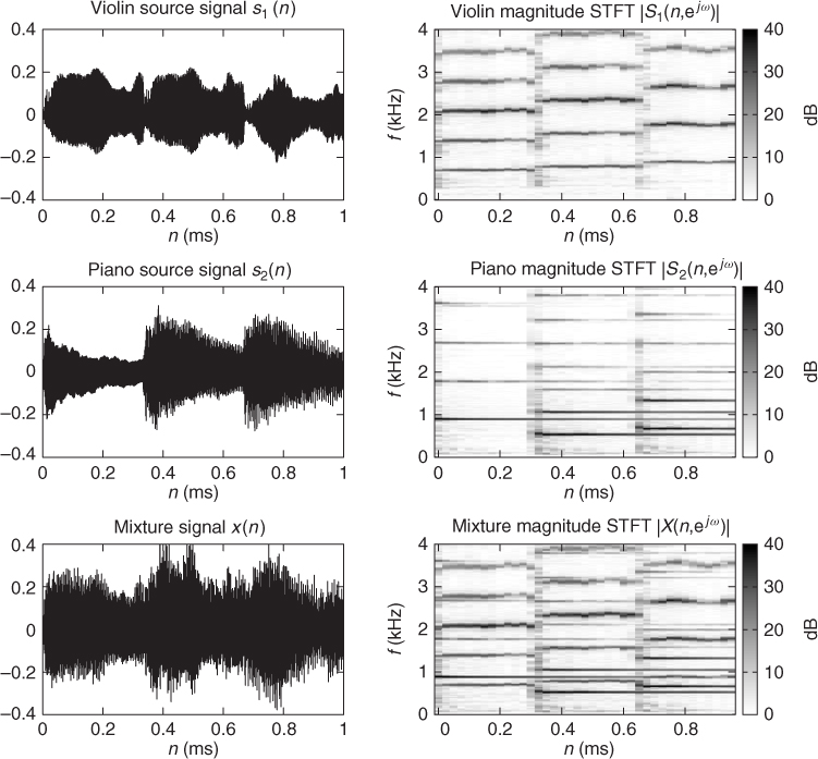
Despite its accurate reproduction of the mixing process, the time domain signal representation (14.2) is generally considered as inconvenient for sound source separation, since all sources except silent ones contribute to each sample xi(n) of the mixture signal. Time-frequency representations are preferred, since they decrease the overlap between the sources and simplify the modeling of their characteristics. Indeed, all sources are typically characterized by distinct pitches or spectra in a given time frame and by distinct dynamics over time, so that one or two predominant sources typically contribute to each time-frequency bin. This property, known as sparsity, makes it easier to estimate their contributions and subsequently separate them. This phenomenon is illustrated in Figure 14.1, where the features of a violin source and a piano source are hardly visible in the mixture signal in the time domain, but are easily segregated in the time-frequency domain.
Figure 14.1 Time vs. time-frequency representation of a single-channel mixture of a violin source and a piano source.
Although perceptually motivated representations have been employed [WB06], the most popular time-frequency representation is the Short Time Fourier Transform (STFT), also known as the phase vocoder, which is the subject of Chapter 7. The mixing process can then be modeled directly over the STFT coefficients using the time-frequency filtering algorithm described in that chapter. However, this exact algorithm requires the window length N to be larger than twice the length of the mixing filters, that is typically on the order of several hundred milliseconds, while the optimal window length in terms of sparsity is on the order of 50 ms [YR04]. Also it introduces a dependency between the source STFT coefficients at different frequencies due to zero-padding, which makes them more complex to estimate. Approximate time-frequency filtering based on circular convolution is hence used instead. Denoting by Xi(n, ejω) and Sm(n, ejω) the complex-valued STFT coefficients of the ith mixture channel and the mth source in time frame n and at normalized frequency ω and by Aim(ejω) the frequency domain mixing coefficients corresponding to the mixing filter aim(τ), the mixing process is approximately modeled as [SAM07]
14.3 
Denoting by X(n, ejω) the I × 1 vector of mixture STFT coefficients and by S(n, ejω) the M × 1 vector of source STFT coefficients, the mixing process can be equivalently expressed as
where A(ejω) is the I × J matrix of mixing coefficients called mixing matrix. Source separation amounts to estimating the STFT coefficients Sm(n, ejω) of all sources and transforming them back to the time domain using overlap-add STFT resynthesis.
Quality Assessment
Before presenting actual source separation techniques, let us briefly introduce the terms that will be used to describe the quality of the estimated sources in the remainder of this chapter. In practice, perfect separation is rarely achieved, e.g., because the assumptions behind source separation algorithms are not exactly met in real-world situations. The level of the target source is then typically increased within each estimated source signal, but distortions remain, compared to the ideal target source signals. One or more types of distortion can arise depending on the algorithm [VGF06]: linear or nonlinear distortion of the target source such as e.g., missing time-frequency regions, remaining sounds from the other sources and additional artifacts taking the form of time- and frequency-localized sound grains akin to those observed in denoising applications (see Chapter 7). These three kinds of distortion will be called target distortion, interference and musical noise, respectively. Minimizing interference alone often results in increasing musical noise, so that a suitable trade-off must be sought, depending on the application. For instance, musical noise is particularly annoying and must be avoided at all costs in hearing-aid applications.
14.1.2 Beamforming and Frequency Domain Independent Component Analysis
Separation via Unmixing Filter Estimation
One of the earliest paradigms for source separation is obtained by in estimating the sources by applying a set of appropriate multi-channel unmixing filters to the mixture. In the time-frequency domain, this amounts to computing the estimated STFT coefficients ![]() of the sources as [BW01]
of the sources as [BW01]
where Wmi(ejω) are complex-valued unmixing coefficients. With similar notations to above, this can be expressed in matrix form as
where W(ejω) is the J × I unmixing matrix.
These filters act as spatial filters that selectively enhance or attenuate sounds depending on their spatial position. In order to understand how these filters can be designed to achieve source separation, let us consider first the simple case of a two-channel mixture of two sources recorded from omnidirectional microphones. The extension of this approach to more than two channels and two sources is discussed later, in Section 14.1.3. Since each interfering source generates a large number of echoes at distinct positions, sounds coming from all of these positions should be canceled. Under the assumption that these positions are far from the microphones relative to the wavelength, sound from a given position will arrive at the second microphone with little attenuation relative to the first microphone, but with a delay δ that is approximately equal to
14.7 ![]()
where d is the microphone spacing in m, fS the sampling frequency in Hz, c the speed of sound i.e., about 344 ms−1 and θ the sound direction of arrival (DOA) relative to the microphone axis oriented from the second to the first microphone. Since the frequency response associated with delay δ is equal to e−jωδ, the directivity pattern of the unmixing filters Wmi(ejω) associated with source p, that is their magnitude response to a sound of normalized frequency ω with DOA θ, is given by [BW01]
Note that distance or elevation do not enter into account, provided that the distance is large enough, so that all sounds located on the spatial cone corresponding to a given DOA are enhanced or attenuated to the same extent.
Beamforming
Expression (14.8) allows it to design the filters so as to achieve suitable directivity patterns. Let us assume for a moment that the DOAs θ1 and θ2 of both sources are known and that we aim to extract the first source. A first simple design is obtained by in setting
14.9 ![]()
14.10 ![]()
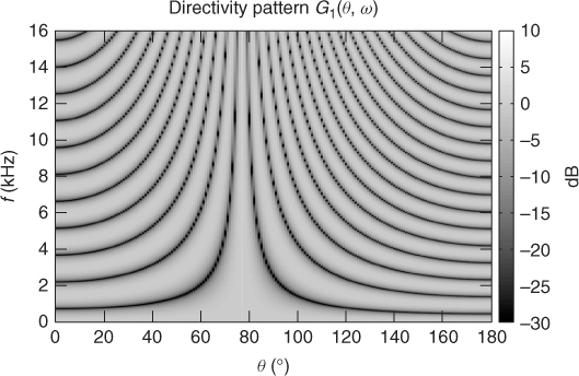
This design, called the delay-and-sum beamformer [BW01], adjusts the delay between the two microphone signals before summing them so that they are perfectly in phase for sounds with DOA θ1, but tend to be out of phase for sounds with other DOAs. The directivity pattern corresponding to this design is depicted in Figure 14.2. Sounds within a beam around the target DOA are enhanced. However, the width of this beam increases with decreasing frequency and it covers the whole space in the range below 400 Hz with the considered microphone spacing of d = 30 cm. Sidelobe beams also appear with a regular spacing at each frequency, so that the interfering source is cancelled at certain frequencies only. This results in an average enhancement of 3 dB.
Figure 14.2 Directivity pattern of the two-channel delay-and-sum beamformer pointing to a target source at θ1 = 77° with a microphone spacing of d = 30 cm.
A more efficient design, called the null beamformer [BW01], is obtained by in setting
14.11 ![]()
14.12 ![]()
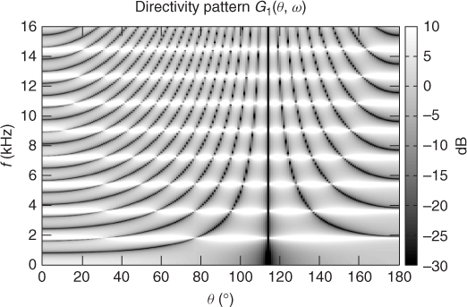
The numerator of this expression adjusts the delay between the two microphone signals so that sounds with DOA θ2 are in antiphase, while the denominator adjusts the gain so as to achieve a flat response to sounds with DOA θ1. The resulting directivity pattern shown in Figure 14.3 confirms that direct sound from the interfering source is now perfectly notched out, while direct sound from the target source is not affected. Note that the notch at θ2 is extremely narrow so that precise knowledge of θ2 is crucial. Also, sidelobes still appear so that echoes of the interfering source are not canceled. Worse, sounds from almost all DOAs are strongly enhanced at frequencies that are multiples of 1.8 kHz with the considered microphone spacing and source DOAs. Indeed, both source DOAs result in similar phase differences between microphones at these frequencies, i.e., ![]() , so that the numerator tends to cancel the target source together with the interfering source and a strong gain must be applied via the denominator to compensate for this. Precise knowledge of θ1 is therefore also crucial, otherwise the target source might become strongly enhanced or attenuated at nearby frequencies.
, so that the numerator tends to cancel the target source together with the interfering source and a strong gain must be applied via the denominator to compensate for this. Precise knowledge of θ1 is therefore also crucial, otherwise the target source might become strongly enhanced or attenuated at nearby frequencies.
Figure 14.3 Directivity pattern of the two-channel null beamformer for a target source at θ1 = 77° and an interfering source at θ2 = 114° with a microphone spacing of d = 30 cm.
The delay-and-sum beamformer and the null beamformer are both fixed designs, which do not depend on the data at hand, except from the source DOAs. More robust adaptive designs have been proposed to attenuate echoes of the interfering source together with its direct sound. For example, the linearly constrained minimum variance (LCMV) beamformer [BW01] minimizes the power of the source signals estimated via (14.5), which is equal to the power of direct sound from the target plus that of echoes and interference, while guaranteeing a flat response over the target DOA. This beamformer can be interpreted in a statistical framework as achieving maximum likelihood (ML) estimation of the sources under the assumption that the sum of all interfering sounds has a stationary Gaussian distribution. Its implementation via the so-called generalized sidelobe canceller (GSC) [BW01] algorithm does not necessitate knowledge of the interfering source DOA anymore, but still requires precise knowledge of the target DOA. In realistic scenarios, this information is not available and must be estimated from the mixture signal at hand. State-of-the-art source localization algorithms e.g., [NSO09] are able to address this issue in anechoic environments, but their accuracy drops in moderately to highly reverberant environments, so that the separation performance achieved by beamforming drops as well.
Frequency Domain Independent Component Analysis
In order to understand how to circumvent this seemingly bottleneck issue, let us come back to the matrix expression of the mixing and unmixing processes in (14.4) and (14.6). By combining these two equations, we get ![]() . Therefore, if the mixing filters were known, choosing the unmixing coefficients as
. Therefore, if the mixing filters were known, choosing the unmixing coefficients as
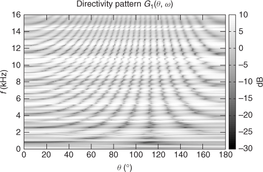
would result in perfect separation i.e., ![]() in the limit where time-frequency domain approximation of the mixing process is valid and A(ejω) is invertible. In practice, A(ejω) can be singular or ill-conditioned at the frequencies for which the sources result in similar phase and intensity differences between microphones. The directivity pattern corresponding to these optimal unmixing coefficients is illustrated in Figure 14.4 in the case of a concert room recording. Deviations compared to Figure 14.3 are clearly visible and due to summation of direct sound and echoes at the microphones, resulting in apparent DOAs different from the true DOAs.
in the limit where time-frequency domain approximation of the mixing process is valid and A(ejω) is invertible. In practice, A(ejω) can be singular or ill-conditioned at the frequencies for which the sources result in similar phase and intensity differences between microphones. The directivity pattern corresponding to these optimal unmixing coefficients is illustrated in Figure 14.4 in the case of a concert room recording. Deviations compared to Figure 14.3 are clearly visible and due to summation of direct sound and echoes at the microphones, resulting in apparent DOAs different from the true DOAs.
Figure 14.4 Directivity pattern of the optimal unmixing coefficients for a target source at θ1 = 77° recorded in a concert room in the presence of an interfering source at θ2 = 114° with a microphone spacing of d = 30 cm.
In practice, the mixing filters are unknown, thus the optimal unmixing coefficients must be adaptively estimated from the mixture signal. This can be achieved in a statistical framework by ML estimation of the unmixing coefficients under the assumption that the STFT coefficients of all sources are independent and follow a certain distribution. It can be shown that the ML objective is equivalent to maximizing the statistical independence of the STFT coefficients of the sources, hence this approach is known as frequency domain independent component analysis (FDICA). A range of prior distributions have been proposed in the literature [SAM07, VJA+10], which typically reflect the aforementioned sparsity property of the sources, i.e., the fact that the source STFT coefficients are significant in a few time frames only, within each frequency bin. Note that this statistical framework is very different from that underlying LCMV beamforming, since the sources are now modeled as separate sparse variables instead of a joint Gaussian “noise.”
A popular family of distributions is the circular generalized Gaussian family [GZ10]
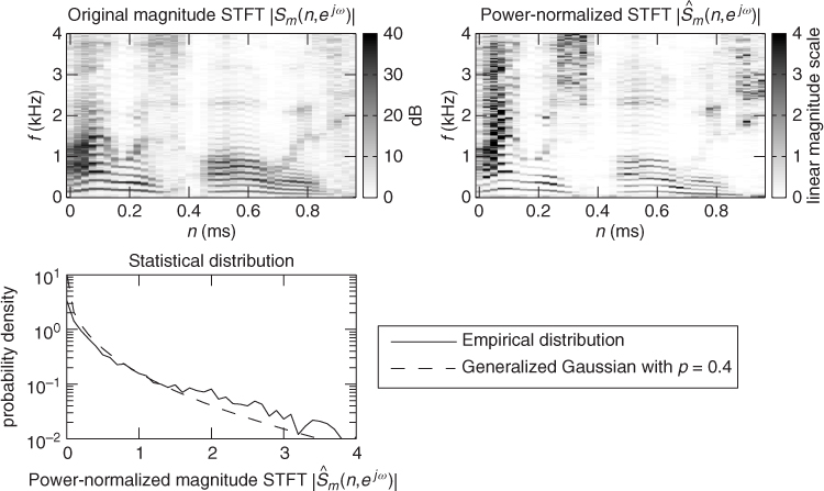
where Γ(.) denotes the function known in mathematics as the gamma function. The scale and shape parameters β and p govern, respectively, the average magnitude and the sparsity of the source STFT coefficients. The smaller p, the more coefficients concentrate around zero. Distributions with shape parameter p < 2 are generally considered as sparse and those with p > 2 as non-sparse with respect to the Gaussian distribution over the magnitude STFT coefficients associated with p = 2. In the absence of prior information about the spectral shape of the sources, the scale parameter β is typically fixed so that the coefficients have unit power. Figure 14.5 shows that this distribution with p = 0.4 provides a very good fit of the distribution of a speech source after power normalization in each frequency bin. The shape parameter value p = 1, which results in the slightly less sparse Laplacian distribution, is nevertheless a popular choice [SAM07].
Figure 14.5 Distribution of the power-normalized magnitude STFT coefficients of a speech source compared to the generalized Gaussian distribution with shape parameter p = 0.4.
The likelihood of the observed mixture signal is obtained by multiplying the probability density (14.14) over all sources, all time frames and all frequency bins. ML estimation of the unmixing coefficients is then equivalent to solving the following optimization problem:
where ![]() implicitly depends on Wmi(ejω) via (14.5). This problem may be addressed using a range of algorithms, that rely on principles of optimization theory beyond the scope of this chapter. Readers may refer to [SAM07] for details.
implicitly depends on Wmi(ejω) via (14.5). This problem may be addressed using a range of algorithms, that rely on principles of optimization theory beyond the scope of this chapter. Readers may refer to [SAM07] for details.
Two additional problems remain. Firstly, since the scale parameter β is constant over all frequency bins, the resulting sources have a flat average spectrum. This scaling indeterminacy of FDICA may be circumvented by exploiting more advanced models of the source spectra or by multiplying the estimated source STFT coefficients by the mixing coefficients derived from the unmixing coefficients via (14.13) so as to estimate the contribution of each source to one or more mixture channels instead of the original source. Secondly, since the model (14.14) is identical for all sources, the sources can be estimated at best up to a random order. This permutation indeterminacy of FDICA can be addressed to a certain extent by exploiting more advanced models of the source spectra or by estimating approximate source DOAs and permuting the unmixing coefficients so that the resulting directivity patterns match the null beamformer pattern in Figure 14.3 as closely as possible. Again, see [SAM07] for details.
14.1.3 Statistically Motivated Approaches for Under-determined Mixtures
We have seen that null beamforming or preferably FDICA can be employed to separate a two-channel mixture of two sources. At this stage, most readers will undoubtedly wonder how these methods generalize to more channels and more sources. As it turns out, these algorithms can be extended to any number of sources and channels. However, they are efficient only when the number of sources is equal to or smaller than the number of channels. Indeed, the number of independent spatial notches corresponding to any set of unmixing filters is at most equal to the number of channels. This can be seen in Figure 14.3 where the unmixing coefficients may be chosen so as to form one notch per frequency in the direction of the interfering source in a two-channel mixture, but other notches due to sidelobes cannot be independently adjusted. Mixtures satisfying this constraint are called determined mixtures.
In the remainder of this chapter, we shall focus on under-determined mixtures, which involve more sources than mixture channels and occur more often in practice. The separation of such mixtures requires a novel paradigm: instead of estimating unmixing filter coefficients, one now wants to estimate the mixing coefficients and the source STFT coefficients directly. Again, this can be addressed in a statistical framework by specifying suitable statistical models for the mixing coefficients and the source STFT coefficients. In practice, for historical reasons, most methods rely on a statistical model of the source STFT coefficients, but adopt a simpler deterministic model for the mixing coefficients based on e.g., perceptual considerations.
Two categories of models have been studied so far, depending on the number of channels. In a multi-channel mixture, spatial information still helps to separate the sources so that weak source models are sufficient. Sparse distributions of the source STFT coefficients have been used in context together with learned mapping functions between the source DOAs and the mixing coefficients. An example algorithm relying on such distributions will be presented in Section 14.2. In a single-channel mixture, spatial information is no more available so that more accurate models of the source STFT coefficients are needed. Example algorithms relying on such models will the described in Section 14.3.
14.1.4 Perceptually Motivated Approaches
The ability to locate and separate sound sources is well developed among humans and animals who use this feature to orient themselves in the dark or to detect potential sources of danger. The field of computational auditory scene analysis (CASA) studies artificial systems able to mimic this localization-separation process. These approaches clearly represent a shift in the paradigm where, rather than modeling the sound production process, focus is in modeling the spatial sound perception processes.
A simple task in source localization is to detect, to a good degree of approximation, the DOA of the source waves from the signals available at the two ears. To a certain extent, humans are able to perform this task even if one of the two ears is obstructed or not functioning, i.e., from monaural hearing. Several models have been conceived to explain binaural perception, which are rooted in the work by Jeffress [JSY98] on the analysis of interaural time difference (ITD) by means of a neuronal coincidence structure, where nerve impulses derived from each of the two ears, stimuli travel in opposite directions over delay lines. This model transforms time information into space information since a nerve cell is excited only at the position on the delay lines where the counter-traveling impulses meet.
Back at the beginning of last century, the ITD together with the interaural level difference (ILD) were considered as the principal spatial hearing cues by Lord Rayleigh, who developed the so-called duplex theory of localization. According to this theory, validated by more recent experimentation, ITDs are more reliable at lower frequencies (roughly below 800 Hz), while ILDs perform better at higher frequencies (roughly above 1.6 kHz). This is due to the fact that the wavelength associated with low audio frequencies is larger than the distance between the ears (typically 12–20 cm). In this case, the perturbation at the two ears is mainly characterized by phase differences with almost equal levels. On the other hand, at higher frequencies, the head is shadowing the perturbation reaching one of the ears, thus introducing relevant ILDs for sound sources that are not placed directly in the frontal direction of the listener. In real measurements, ITDs and ILDs are the result of multiple reflections, diffractions and resonances generated in the head, torso and external ears of the listener. Consequently, the interpretation and use of ITD and ILD as cues for DOA detection is less simple and error prone [Bla01, Gai93, Lin86, ST97].
In perceptually motivated source separation methods, the binaural signals are first input to a cochlear filter bank. The sources are separated by processing linearly or non-linearly the signal in perceptual frequency bands. Typical non-linear processing includes half-wave rectification or squaring followed by low-pass filtering [FM04]. ITD and ILD are also estimated within perceptual bands and used as cues for the separation.
While the accurate modeling of binaural hearing is essential to the understanding of auditory scene analysis as performed by humans or animals, several approaches to sound source localization and separation based on spatial cues were derived for the sole purpose of processing audio signals. In this case, the proposed algorithms are often only crudely inspired by human physiological and perceptual aspects. The ultimate goal is to optimize performance, without necessarily adhering to biological evidence. For example, the frequency resolution at which ITD and ILD cues can be estimated can go well beyond that of the critical frequency bands of the cochlear filter bank.