14.2 Binaural Source Separation
In binaural separation, the various sources are segregated according to spatial cues extracted from the signals available at both ears. This is the case for signals transduced by the microphones of a two-ear hearing-aid system or of the signals available at the microphones in the artificial ears of a dummy head. The type of apparatus is irrelevant, as long as human-like head shadowing is present in-between the microphones. A common strategy is to first detect and discern sources based on the DOA of waves, which is the object of Section 14.2.1, and then to build suitable time-frequency masks in a two-channel STFT representation of the binaural signal in order to demix them. Each mask, which can be binary or continuous valued with arbitrary values in [0, 1], coarsely represents the time-frequency profile of a given source. Due to energy leakage in finite sliding window time-frequency analysis, the masks are bound to cover broader bands than the ideal time-frequency tracks. The estimation of proper masks is the subject of Section 14.2.2. The masks are multiplicatively applied to both STFT channels and the transforms inverted. The ideal outcome is a set of binaural signals, each representing the sound of a single source spatially placed at the corresponding DOA.
14.2.1 Binaural Localization
An important aspect of binaural localization is the estimation of the DOA in terms of azimuth and elevation. Together with the range information (distance from the source), it provides full knowledge of the coordinates of the source. However, we shall confine ourselves to estimates of the azimuth only. Estimates of the range are difficult in closed spaces and if the distance of the source to the listener is not large. Estimates of the elevation are affected by larger error, even in the human hearing system. The so-called cones of confusion [Bre90], show large uncertainty on the elevation of the source, while azimuth uncertainty as sharp as ![]() is common in humans. It must be pointed out that the azimuth resolution depends on the angle, with lateral directions providing less sharp results.
is common in humans. It must be pointed out that the azimuth resolution depends on the angle, with lateral directions providing less sharp results.
In order to estimate the azimuth of the source one can explore spatial cues such as ILD and ITD. For any given source and at any given time, the ILD is the difference in level as received at the ears. Given the STFT of the left and right ear signals, ![]() and
and ![]() , respectively, one can estimate the ILD at any angular frequency ω and time interval indexed by n, where the signal energy is above a certain threshold, as follows:
, respectively, one can estimate the ILD at any angular frequency ω and time interval indexed by n, where the signal energy is above a certain threshold, as follows:
Basically, the ILD estimate is the difference in dB of the amplitudes in the two channels as a function of frequency and averaged over the STFT analysis interval [nN, ..., nN + M − 1], where the integers N and M respectively denote hop-size and window length of a discrete time STFT.
For any given source and at any given time, the ITD is defined as the time shift of the two signals received at the ears. This time shift could be measured, e.g., by finding a local maximum of the two signals, cross-correlation. However, in the time-frequency paradigm we adopted for the whole localization-separation process, for each angular frequency ω one can estimate the ITD from the STFT of the two ear signals, as follows:
The ITD is estimated from the phase difference of the two ear signals. In fact, through division by ω, it corresponds to a phase delay measurement. Since the phase is defined modulo 2π, there is an ambiguity in the estimate that is a multiple of this quantity, which justifies the term 2πp in (14.17), where p is any integer.
By the nature of the problem, ITD estimates are sharper at lower frequencies, where the effect of phase ambiguity is minimized, while ILD estimates are sharper at high frequencies, i.e., at wavelengths much shorter than the distance between the ears.
Localization Using HRTF Data or Head Models
Azimuth estimation from ITD and ILD can be performed by means of table lookup, using a set of measured HRTFs for a given individual. Given the measurements ![]() and
and ![]() of the subjective HRTF for the right and left ears as a function of the azimuth θ and angular frequency ω, one can form the following tables:
of the subjective HRTF for the right and left ears as a function of the azimuth θ and angular frequency ω, one can form the following tables:
and
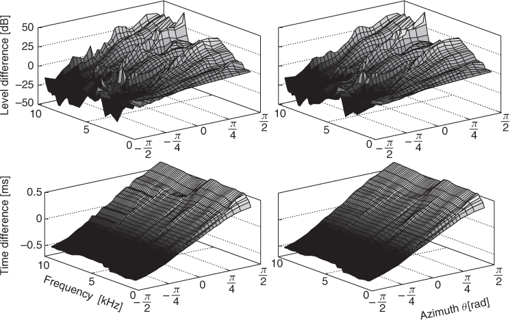
for the azimuth lookup, respectively, from ILD and ITD estimates. As shown in Figure 14.6 left column, the measured HRTF tables are quite noisy, depending on the details of multiple head—torso wave reflection. It is practice to smooth these tables along the azimuth axis, as shown in Figure 14.6 right column; we will continue to use the same symbols as in (14.18) and (14.19) to denote the smoothed tables.
Figure 14.6 Spatial cues from HRTF measurements; Left: Unsmoothed estimates, Right: Estimates smoothed along azimuth axis; Top: Level differences; Bottom: Time differences. Figure reprinted with IEEE permission from [RVE10].
For any frequency, given an STFT-based estimate ΔLn(ω) for the level difference as in (14.16), the azimuth θ can be estimated by finding in (14.18) which value of θ provides the measured ILD. We denote this estimate by θL, n(ω).
Similarly, given an STFT-based estimate ΔTn, p(ω) for the time difference as in (14.17), the azimuth can be estimated by finding in (14.19) which value of θ provides the measured ITD. The time-difference estimate depends on an arbitrary integer multiple p of 2π. Therefore, for any fixed-frame index n and angular frequency ω, each ITD estimate is compatible with a countable infinity of azimuth estimates θT, n, p(ω). However, assuming that the phase difference of the HRTFs does not show large discontinuities across azimuth and that the phase difference at zero azimuth is as small as possible, i.e., zero, it is possible to resolve the phase ambiguity by unwrapping the phase difference of the right and left HRTFs along the azimuth. Even when this ambiguity is resolved, there can still be several values of θ providing the same ILD or ITD values in the HRTF lookup. While smoothing tends to partially reduce ambiguity, majority rules or statistical averages over frequency or other assumptions can be used to increase the reliability of the azimuth estimate.
Usually, the duplex theory is applied here to choose among the estimates as a function of frequency. At low frequencies, the estimate ΔTs, 0(θ, ejω) is selected for the azimuth lookup estimates from unwrapped phase difference, while at high frequencies ΔLs(θ, ejω) is selected. In Section 14.2.1 a procedure for azimuth estimate jointly employing ITD and ILD is described.
Given a head radius of r meters, the cut-off frequency fc to switch from ITD- to ILD-based azimuth estimates can be estimated as the inverse of the time for the sound waves to travel from ear to ear along the head semicircle, i.e., ![]() , where c ≈ 344 ms−1 is the speed of sound in air. Approximately a cut-off frequency of 1.6 kHz is selected to switch from ITD- to ILD-based estimates when the head radius is not known.
, where c ≈ 344 ms−1 is the speed of sound in air. Approximately a cut-off frequency of 1.6 kHz is selected to switch from ITD- to ILD-based estimates when the head radius is not known.
The discussed azimuth estimation lookup procedure requires knowledge of the individual HRTFs. When these are not known, it is possible to resort to a slightly less accurate estimation procedure which makes use of average ILD and ITD, respectively obtained from (14.18) and (14.19) by averaging over several individuals in a database of HRTFs. It can be shown [RVE10] that the performance of the averaged model is comparable with that of the method based on individual transfer functions.
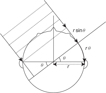
At the cost of slightly reduced performance, it is possible to eliminate the need for HRTF-based lookup tables in azimuth estimates. In fact, from simple geometric considerations [WS54], as shown in Figure 14.7 for an idealized face represented by a circular section of radius r, the two ears, path-length difference for a wave reaching from DOA θ is not only due to an “in air” term rsinθ, but also to the arc length rθ of a curved path along the face, yielding
Due to the fact that the head is not perfectly spherical, the measured ITD is slightly larger than the values in (14.20), especially at low frequencies. A more accurate model, discussed in [RVE10], scales the ITD model (14.20) by a frequency and, possibly, subject-dependent scaling factor αs(ω), to obtain
Given a measure of the ITD ΔTs(θ, ω), in order to produce an estimate for the azimuth θ one needs to invert (14.21), which can be achieved by polynomial approximation [RVE10].
Figure 14.7 Path-length difference model for the ITD based on head geometry.
The ILD is a much more complex function of frequency. However, based on the observation of a large number of HRTFs, the following model [RVE10] can be shown to capture its main features when the sources are at large distances (over 1.5 m) from the listener;
where βs(ω) is again a frequency and, possibly, subject-dependent scaling factor. Inversion of (14.22) in order to produce an estimate for the azimuth does not present any problems.
Localization Using ITD, ILD and IC
Since both the ILD and the ITD are related to the azimuth, they can be jointly employed in order to improve the azimuth estimates. The noisy ΔLn(ω) provides a rough estimate of the azimuth for each left/right spectral-coefficient pair. This ILD estimate can be used in order to select the most reasonable value for the parameter p in the ITD estimate, which is the one for which the ILD- and ITD-based estimates provide the closest value for the azimuth. Formally, this is given by
14.23 ![]()
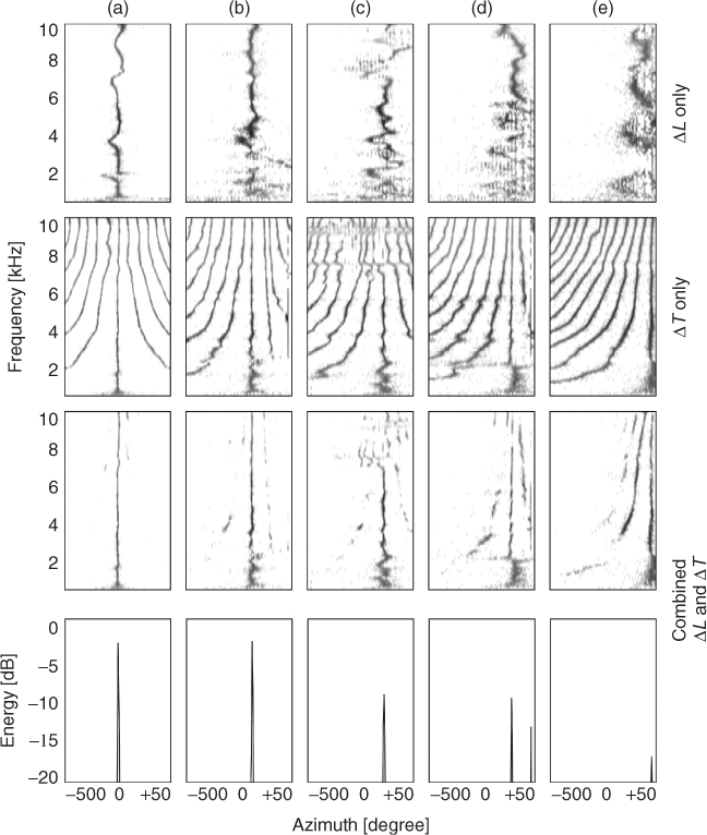
Comparative experimental results obtained by ILD only, ITD only and the joint method are shown in Figure 14.8 for a single white-noise source located at angles 0°, 15°, 30°, 45° and 65°. Extensive performance evaluation of the joint ILD-ITD azimuth estimates can be found in [RVE10].
Figure 14.8 2D time histograms of azimuth estimates, in terms of azimuth and frequency, for five different heads and azimuth angles an 0°, 15°, 30°, 45° and 65°, (a)–(e), respectively. First row: based on ILD only. Second row: based on ITD only. Third row: based on combined evaluation of ILD and ITD. Bottom row: marginal histograms obtained by summing the combined ITD-ILD evaluation over all frequencies. Figure reprinted with IEEE permission from [RVE10].
In the presence of one source only, the two ear signals xL and xR approximately are two delayed and amplitude-scaled versions of the same signal. In that case, the interaural cross correlation (ICC), defined as the normalized cross-correlation
peaks at a time lag corresponding to the relative delay or global ITD of the two signals. The amplitude of the peak provides a measure of similarity. In the presence of two or more sources with different DOA, the cross-correlation peaks are less distinguishable: since there is more than one characteristic delay, the two ear signals are less similar. The interaural coherence (IC) is defined as the maximum of the normalized cross-correlation of the two ears signals, which is a number between 0 and 1. It is useful to evaluate the ICC in time-frequency, i.e., with xL(n) and xR(n) in (14.24) replaced by the STFTs ![]() and
and ![]() , respectively:
, respectively:
14.25 
where * denotes complex conjugation. In practice, the ICC is smoothed in time [Men10] in order to mitigate the oscillatory behavior due to the STFT finite window length. The corresponding time-frequency IC cue, defined as the amplitude of the maximum of the time-frequency ICC for any fixed frequency, provides a measure of reliability of the ITD and ILD for each frequency channel [FM04], IC being larger if only one source contributes to a given frequency bin. Furthermore, the time-frequency IC can be effectively employed as a cue to improve separation in the presence of time-frequency overlapping sources, where non-binary demixing masks are optimized by maximizing the IC of the separated sources.
14.2.2 Binaural Separation
In Section 14.2.1, methods for the localization of sources in binaural signals are discussed, which are based on DOA discrimination from the STFT of the signals observed at the two ears. The azimuth θ(n, ω) estimated for each left/right pair of spectral coefficients pertains to a narrow-band signal component in a short time interval. The ensemble of azimuth estimates can be employed to obtain separate binaural signals where the spatial information is preserved, but where only one source is present in each, which is the object of this section. Starting from the simple method based on binary masks we then explore the construction of continuous-valued masks based on Gaussian mixtures models of the multi-modal distribution of azimuth estimates. We then illustrate the use of structural assumption in the multi-channel separation of overlapping harmonics.
Binary Masks
At any given time, each prominent peak of the histogram h(θ) obtained by cumulating the azimuth estimates θ(n, ω) over frequency pertains to a different observed DOA. On the assumption that the sound sources are spatially distributed, so that each has a sufficiently distinct DOA as observed by the listener, the number of peaks equals the number of sources. The position of the peak estimates the DOA θk(n) of the corresponding source, where k represents the source index, which can be tracked over time.
Given the azimuth estimates θ(n, ω) and the source azimuths θk(n), a weighting factor Mk(n, ω) can be given for each spectral coefficient. For each source, the separated binaural signal is obtained by multiplying this weighting factor by the STFT of the left and right ear signals followed by STFT inversion. Respectively, the left and right channel STFTs of the kth reconstructed source signal are given by
14.26 
Different approaches can be considered for the definition of the weights. On the assumption that the STFT spectra of the different sources do not overlap significantly, i.e., on the window-disjoint orthogonal (WDO) assumption [YR04]. In this case, only one source contributes significant energy to a given spectral coefficient so that each spectral coefficient can be exclusively assigned to that source. Binary weights can be efficiently employed in this case. A possible strategy is to assign each spectral coefficient to the source whose azimuth estimate is closest. This is formalized by the following choice of weights
This weight system can be considered as a spatial window in which the coefficients are assigned to a given source according to the closeness of direction. However, this choice of weights can lead to artifacts due to the fact that azimuth estimates that are very far from the estimated azimuth of any source are unreliable. Therefore, the corresponding STFT coefficients should not be arbitrarily assigned to a source in this case. It may be better to consider these estimates as outliers and assign to a given source only those STFT coefficients for which the corresponding azimuth estimates lie in a window of width W from the estimated source azimuth. This is formalized by the following choice of weights:
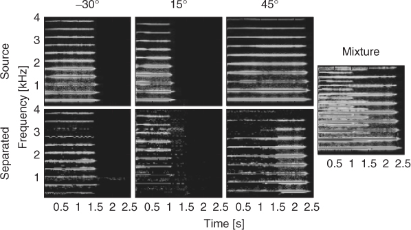
The result of the separation of three trombone sources, each playing a different note, located at −30°, 15° and 45° are shown in Figure 14.9, together with the spectrogram displayed in Figure 14.10. Artifacts are visible and audible especially in the attack area and during silence. Smoothing in the time direction can effectively reduce artifacts due to mask switching. However, in performed music, more severely than in speech, the overlap of the sources in time-frequency is not a rare event. In fact, musicians are supposed to play with the same tempo notes that are harmonically related, which means that several partials of the various instruments are shared within the same time interval. This results in artifacts of the separation when binary weighting of either of the forms (14.27) and (14.28) is enforced. One way to reduce these artifacts is to enforce non-binary weighting in which the energy of time-frequency bins is distributed among two or more overlapping sources, with different weights. Even in the ideal case where one can guess the exact weights, the separation continues to be affected by error in view of the fact that the phase of the signal components is also important, but not taken into consideration. The relative phase of the source components overlapping in the same bin also affects the total energy by interference.
Figure 14.9 Binary mask separation of three trombone sources located at −30°, 15° and 45°: time domain.
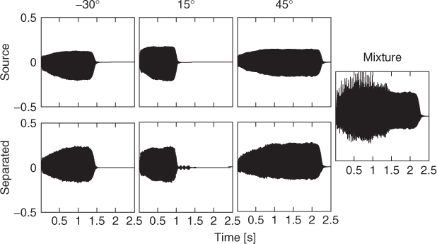
Figure 14.10 Binary mask separation of three trombone sources located at −30°, 15° and 45°: spectrograms (gray-scale magnitude).
Gaussian Mixture Model
In theory, in the case of a single source all frequencies should give the same azimuth, exactly corresponding to the source position θ. However, in practice, the violation of the WDO assumption, the presence of noise and estimation errors make things a little more complicated. As a first approximation, we consider that the energy of the source is spread in the power histogram following a Gaussian distribution centered at the theoretical value θ. The Gaussian nature of the distribution is confirmed by the well-known central limit theorem as well as practical experiments. In this context, the ideal case is a Gaussian of mean θ and variance 0.
In the case of K sources, we then introduce a model of K Gaussians (K-GMM, order-K Gaussian mixture model)
14.29 
where Γ is a multi-set of K triples ![]() that denotes all the parameters of the model; πk, μk and
that denotes all the parameters of the model; πk, μk and ![]() indicate respectively the weight, the mean and the variance of the kth Gaussian component described mathematically by
indicate respectively the weight, the mean and the variance of the kth Gaussian component described mathematically by
14.30 
We are interested in estimating the architecture of the K-GMM, that is the number of sources K and the set of parameters Γ, to be able to setup the separation filtering.
Unmixing Algorithm
In the histogram h(θ), we observe local maxima whose number provides an estimation of the number of sources in the mixture. The abscissa of the kth local maximum reveals the location θk of the kth source. However, in practice, to avoid spurious peaks, we must deal with a smoothed version of the histogram and consider only significant local maxima–above the noise level. Informal experiments show that the estimated source number and location are rather good. This gives the model order K and a first estimation of the means of the Gaussians (μk in Γ). This estimation can be refined and completed–with the variances ![]() and the weights πk–for example by the EM algorithm.
and the weights πk–for example by the EM algorithm.
Expectation maximization (EM) is a popular approach to estimate parameters in mixture densities, given a data set x. The idea is to complete the observed data x with an unobserved variable y to form the complete data (x, y), where y indicates the index of the Gaussian component from which x has been drawn. Here, the role of x is played by the azimuth θ, taking values in the set of all discrete azimuths covered by the histogram. We associate θ with its intensity function h(θ) (the histogram). The role of y is played by k ∈ {1, ![]() , K}, the index of the Gaussian component θ should belong to.
, K}, the index of the Gaussian component θ should belong to.
The EM algorithm proceeds iteratively, at each iteration the optimal parameters that increase locally the log-likelihood of the mixture are computed. In other words, we increase the difference in log-likelihood between the current with parameters Γ and the next with parameters Γ′. This log-form difference, noted Q(Γ′, Γ), can be expressed as
14.31 
We can then reformulate ![]() like this:
like this:
14.32 
The concavity of the log function allows us to lower bound the Q(Γ′, Γ) function using the Jensen's inequality. We can then write
14.33 ![]()
where PK(k|θ, Γ) is the posterior probability, the degree to which we trust that the data was generated by the Gaussian component k, given the data; it is estimable with the Bayes rule
The new parameters are then estimated by maximizing the lower bound with respect to Γ;
Increasing this lower bound results automatically in an increase of the log-likelihood, and is mathematically easier. Finally, the maximization of Equation (14.35) provides the following update relations (to be applied in sequence, because they modify–update–the current value with side-effects, thus the updated value must be considered in the subsequent relations):
The performance of the EM depends on the initial parameters. The first estimation parameter should help to get the around the likelihood local maxima trap. Our EM procedure operates as follows:
1. Initialization step
- initialize K with the order of the first estimation
- initialize the weights equally, the means according to the first estimation, and the variances with the data variance (for the initial Gaussians to cover the whole set of data):

- set a convergence threshold

2. Expectation step
- compute PK(k|θ, Γ) with Equation (14.34)
3. Maximization step
Finally, to separate the sources, a spatial filtering identifies and clusters bins attached to the same source. Many methods, like DUET, separate the signals by assigning each of the time-frequency bins to one of the sources exclusively. We assume that several sources can share the power of a bin, and we attribute the energy according to a membership ratio–a posterior probability. The histogram learning with EM provides a set of parameters for the Gaussian distribution that characterizes each source. These parameters are then used to parameterize automatically a set of spatial Gaussian filters. In order to recover each source k, we select and regroup the time-frequency bins belonging to the same azimuth θ. We use the parameters issued from the EM-component number k, and the energy of the mixture channels is allocated to the (left and right) source channels according to the posterior probability. More precisely, we define the following mask for each source:
14.39 ![]()
if ![]() , and 0 otherwise. This mask limits the fact that the tail of a Gaussian distribution stretches out to infinity. Below the threshold
, and 0 otherwise. This mask limits the fact that the tail of a Gaussian distribution stretches out to infinity. Below the threshold ![]() (expressed in dB, and set to −20 in our experiments), we assume that a source of interest does not contribute anymore. For each source k, the pair of short-term spectra can be reconstructed according to
(expressed in dB, and set to −20 in our experiments), we assume that a source of interest does not contribute anymore. For each source k, the pair of short-term spectra can be reconstructed according to
14.40 ![]()
14.41 ![]()
Experimental Results
First, we synthesized binaural signals by mixing monophonic source signals filtered through the HRTFs of a given individual corresponding to various azimuths using the HRTF-based technique, then we applied the EM-based unmixing algorithm described in the previous section.
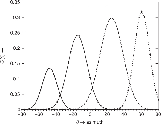
A result of demixing is depicted in Figure 14.11 for a two-instrument mixture: xylophone at −55° and horn at −20°; their original spectrograms are shown in Figure 14.12. In the time domain, the xylophone rhythm is respected, its signal looks amplified and its shape is preserved. Perceptively, the demixed xylophone is very similar to the original one. Also, for the horn, we must tolerate some interference effects, and the spectrograms are partly damaged. A portion of energy was absorbed by an unwanted source generated from interferences. We also conducted tests on speech samples. The reconstruction quality was good, much better than for long-distance telephone lines. Figure 14.13 shows the power histogram for the localization of four instruments in a binaural mixture. This histogram, here of size 65, was built using FFTs of N = 2048 samples with an overlap of 50%. Figure 14.14 shows the (normalized) Gaussian mixture model associated to this histogram. Of course, the EM algorithm can also be applied on the raw azimuth estimates ![]() instead of the data stored in the histogram.
instead of the data stored in the histogram.
Figure 14.11 Waveforms of the demixtures (on the right, originals being on the left): xylophone (−55°) (top) and horn (30°) (bottom).
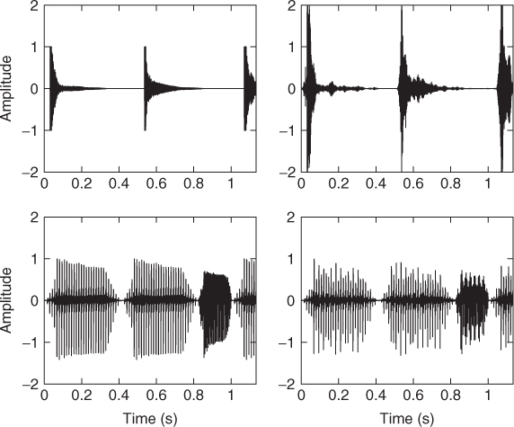
Figure 14.12 Spectrograms of the four sources, from top to bottom: xylophone, horn, kazoo and electric guitar.
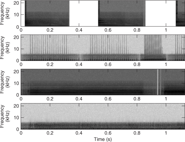
Figure 14.13 Histogram (solid line) and smoother version (dashed line) of the four-source mix: xylophone at −55°, horn at −20°, kazoo at 30° and electric guitar at 65°.
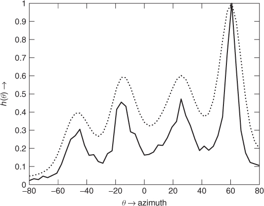
Figure 14.14 GMM (normalized) for the histogram of the four-source mix.
Multi-channel Separation of Overlapping Harmonics
The separation of time-frequency overlapping source components is a very challenging problem. However, in a multi-channel context one can use the sensor signals, together with structural cues, e.g., harmonicity, in order to successfully separate the contributions of the various sources to the shared time-frequency components.
For each bin of the discrete time-frequency spectrum, let us now consider the observed magnitude in this frequency bin as time goes by. If a single stationary sinusoid has amplitude a and frequency exactly equal to the frequency of one of the analysis bin, the observed magnitude STFT at that bin is proportional to the amplitude of the sinusoid.
When two sinusoids are present at the same frequency, then the resulting signal is also a sinusoid of the same frequency (straightforward when considering the spectral domain). More precisely, the complex instantaneous amplitudes of the sinusoids add together as follows:
14.42 ![]()
where ap and ϕp are the amplitude and phase of the p-th sinusoid (p ∈ {1, 2}). Thus, via the Cartesian representation of complex numbers, the corresponding magnitude is
14.43 ![]()
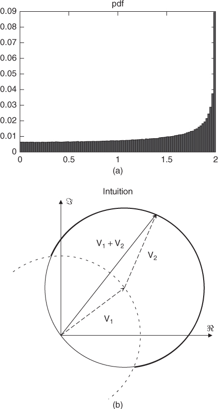
Physically, the addition of two sinusoidal signals, even of the same amplitude a0 (a1 = a2 = a0), is ruled by a nonlinear addition law which gives a maximum of 2a0 (thus ≈ 6 dB above the volume of a0) when the sinusoids are in phase (ϕ1 = ϕ2) and a minimum of 0 when they are opposite phase (ϕ1 = ϕ2 + π). One might intuitively think that all the cases in the [0, 2a0] interval are equiprobable. Not at all! For example, in the case where the initial phases of the sinusoids are independent uniformly distributed random variables over [−π, +π) we have that a ≈ a1 + a2 is the most probable value for the magnitude, as shown in Figure 14.15. The interference of several sinusoids at the same frequency results in one sinusoid. In this situation, it is quite impossible to separate the two sinusoids without additional knowledge. A possible strategy would be to simply ignore time-frequency regions where this interference phenomenon is likely to occur. However, in the case of musical signals, musicians playing in tempo and in harmony often generate frequency overlap at least for some of the partials. Thus, the separated signals would present large time intervals in which all or some of the partials are muted. When properly exploited, structural cues can help disambiguate overlapping partials and provide heuristics for their separation. In fact, under the assumption of quasi-periodicity of the sources, all the signals are nearly harmonic. Although this may seem a particular case of a general inharmonic structure, one can push the methods a little further with simple techniques and minimal side information. In fact, given that at least one of the partials for each source is not completely overlapping in time-frequency with those of the others, one can assume a harmonic structure based on the isolated partials, without additional knowledge of the sources. The overlap of the partials is resolved by assuming that the time envelopes of each partial are similar, with neighboring partials bearing the highest similarity.
Figure 14.15 Interference of two sinusoids of the same frequency and amplitude 1. The signal resulting from the addition of the these two sinusoids is also a sinusoid with the same frequency, but its amplitude depends on the phases of the initial sinusoids. (a) shows histogram illustrating the probability density function of this amplitude (for uniform distributions of the phases). The sum of the amplitudes (2) is the most probable value. (b) gives an intuitive justification. It shows that, considering the sum of the two vectors corresponding to the complex amplitudes of the sinusoids in the complex plane (see Equation (14.15)), its norm is more likely to be greater than 1 (bold line).
A similarity measure was proposed in [HG06], which involved the normalized scalar product of the envelopes;
where Ep(n) and Eq(n) are the time envelopes of two components detected in time-frequency, each obtained by detecting and tracking in time contiguous zones of nonzero energy in adjacent frequency bins. When the envelopes are quite similar, like the ones of adjacent harmonics of a single source, the similarity measure βp, q is close to one. However, when interference among the sources is present, the similarity measure is much lower than 1.
All the sensor signals can be used in the case of multi-channel signals. The problem of separating the overlapping partials can be stated as that of estimating a mixing matrix from a known number of N sources contributing to M distinct measurements of each partial. For the problem to have a reliable solution there must be at least as many sensors as there are overlapping partials in that region. In view of the narrow-band characteristics of the partials, one can model this mixing process in time-frequency by means of constant complex matrices for each partial [HG06] in each frequency bin. For a two-sensor two-sources case of overlapping partials at frequency bin ω we have
14.45 ![]()
where Si(n, ejω), i = 1, 2 represent the STFTs of the original source signals, HL/R, i(ejω) the frequency responses from source i to left/right sensor channel and PL/R(n, ejω) the STFTs of mixed overlapping partials at left and right sensors. The matrix composed by the frequency responses HL/R, i(ejω) is the mixing matrix at frequency bin ω.
In order to proceed with separation, first the envelopes of the other nonoverlapping partials are computed, which are called the model envelopes. Then, for each candidate mixing matrix, its pseudo-inverse is applied to the sensor-mixed partials and the envelopes of the resulting partials are computed. The matrix that gives separated partials with envelopes whose shapes most closely resemble those of the model envelopes is chosen as the estimate of the mixing matrix for that corresponding partial. Thus, the estimate of the mixing matrix is obtained by means of optimization as the one that gives the best match between the separated partials and the model partials according to the criterion (14.44).
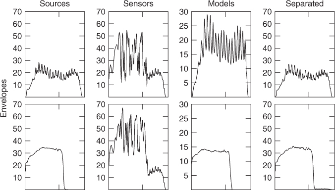
Good experimental results are obtained by using the L1 norm to combine the similarity measures deriving by each partial [Vis04]. An example of separation of overlapping partials from two sources, a violin tone with vibrato and a trombone tone without vibrato, is shown in Figure 14.16, where one can appreciate how closely the envelopes are recovered, together with the fine AM-FM fine structure due to vibrato in the violin tone.
Figure 14.16 Simple example of separation of overlapping partials from two harmonic sources, violin (top row) and trombone (bottom row). Columns from left to right: source envelopes, mixed source envelopes at left and right sensors, model envelopes extracted from nonoverlapping partials at sensor signals, envelopes of separated partials maximizing envelope similarity.