2.5 Basic Delay Structures

2.5.1 FIR Comb Filter

The A network that simulates a single delay is called a FIR comb filter. The input signal is delayed by a given time duration. The effect will be audible only when the processed signal is combined (added) to the input signal, which acts here as a reference. This effect has two tuning parameters: the amount of time delay τ and the relative amplitude of the delayed signal to that of the reference signal. The difference equation and the transfer function are given by

2.58

2.59

2.60

The time response of this filter is made up of the direct signal and the delayed version. This simple time-domain behavior comes along with interesting frequency-domain patterns. For positive values of g, the filter amplifies all frequencies that are multiples of 1/τ and attenuates all frequencies that lie in-between. The transfer function of such a filter shows a series of spikes and it looks like a comb (Figure 2.27), hence the name. For negative values of g, the filter attenuates frequencies that are multiples of 1/τ and amplifies those that lie in-between. The gain varies between 1 + g and 1 − g [Orf96]. The following M-file 2.5 demonstrates a sample-by-sample based FIR comb filter. For plotting the output signal use the command stem(0:length(y)-1,y) and for the evaluation of the magnitude and phase response use the command freqz(y,1).

Figure 2.27 FIR comb filter and magnitude response.

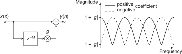
Just as with acoustical delays, the FIR comb filter has an effect both in the time and frequency domains. Our ear is more sensitive to the one aspect or to the other depending on the range in which the time delay is set. For larger values of τ, we can hear an echo that is distinct from the direct signal. The frequencies that are amplified by the comb are so close to each other that we barely identify the spectral effect. For smaller values of τ, our ear can no longer segregate the time events, but can notice the spectral effect of the comb.

2.5.2 IIR Comb Filter

Similar to the endless reflections at both ends of a cylinder, the IIR comb filter produces an endless series of responses y(n) to an input x(n). The input signal circulates in a delay line that is fed back to the input. Each time the signal goes through the delay line it is attenuated by g. It is sometimes necessary to scale the input signal by c in order to compensate for the high amplification produced by the structure. It is implemented by the structure shown in Figure 2.28, with the difference equation and transfer function given by

2.61

2.62

Figure 2.28 IIR comb filter and magnitude response.

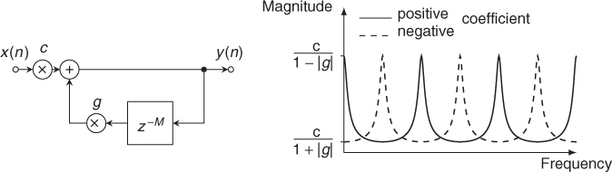
Due to the feedback loop, the time response of the filter is infinite. After each time delay τ a copy of the input signal will come out with an amplitude gp, where p is the number of cycles that the signal has gone through the delay line. It can readily be seen, that |g| ≤ 1 is a stability condition. Otherwise the signal would grow endlessly. The frequencies that are affected by the IIR comb filter are similar to those affected by the FIR comb filter. The gain varies between 1/(1 − g) and 1/(1 + g). The main differences between the IIR comb and the FIR comb is that the gain grows very high and that the frequency peaks get narrower as |g| comes closer to 1 (see Figure 2.28). The following M-file 2.6 shows the implementation of a sample-by-sample based IIR comb filter.

2.5.3 Universal Comb Filter

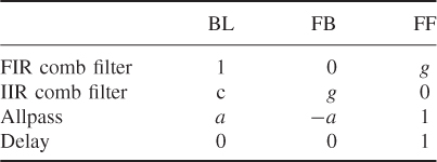
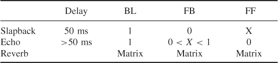
The combination of FIR and IIR comb filters leads to the universal comb filter. This filter structure, shown in Figure 2.29, reverts to an allpass structure in the special case of −BL = FB, FF = 1 (see Figure 2.5), where the one sample delay operator z−1 is replaced by the M sample delay operator z−M. The special cases for differences in feedback parameter FB, feedforward parameter FF and blend parameter BL are given in Table 2.6. M-file 2.7 shows the implementation of a sample-by-sample universal comb filter.

Figure 2.29 Universal comb filter.

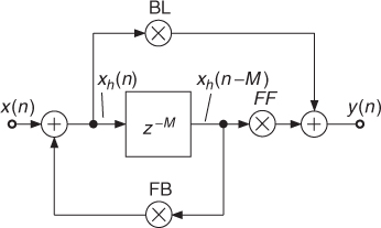
Table 2.6 Parameters for universal comb filter

The extension of the above universal comb filter to a parallel connection of N comb filters is shown in Figure 2.30. The feedback, feedforward and blend coefficients are now N × N matrices to mix the input and output signals of the delay network. The use of different parameter sets leads to the applications shown in Table 2.7.

Figure 2.30 Generalized structure of parallel allpass comb filters.

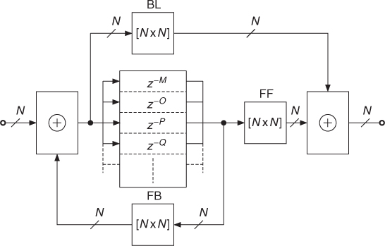
Table 2.7 Effects with generalized comb filter

2.5.4 Fractional Delay Lines

Variable-length delays of the input signal are used to simulate several acoustical effects. Therefore, delays of the input signal with noninteger values of the sampling interval are necessary. A delay of the input signal by M samples plus a fraction of the normalized sampling interval with is given by

2.63

and can be implemented by a fractional delay shown in Figure 2.31.

Figure 2.31 Fractional delay line with interpolation.

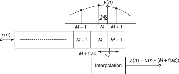
Design tools for fractional delay filters can be found in [LVKL96]. An interpolation algorithm has to compute the output sample y(n), which lies in-between the two samples at time instants M and M + 1. Several interpolation algorithms have been proposed for audio applications:

• Linear interpolation [Dat97b]

  2.64

• Allpass interpolation [Dat97b]

  2.65

• Sinc interpolation [FC98]
• Fractionally addressed delay lines [Roc98, Roc00]
• Spline interpolation [Dis99], e.g., of third order

  2.66

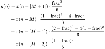
They all perform interpolation of a fractional delayed output signal with different computational complexity and different performance properties, which are discussed in [Roc00]. The choice of the algorithm depends on the specific application.