4.2 Dynamic Range Control

Dynamics processing is performed by amplifying devices where the gain is automatically controlled by the level of the input signal. We will discuss limiters, compressors, expanders and noise gates. A good introduction to the parameters of dynamics processing can be found in [Ear76, pp. 242–248].

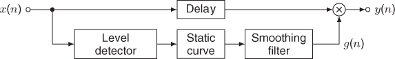
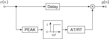
Dynamics processing is based on an amplitude/level detection scheme sometimes called an envelope follower, a static curve to derive a gain factor from the result of the envelope follower, a smoothing filter to prevent too abrupt gain changes and a multiplier to weight the input signal (see Figure 4.7). Optionally, the input signal is delayed to compensate for any delay in the side chain, the lower path in Figure 4.7. Normally, the gain factor is derived from the input signal, but the side chain path can also be connected to another signal for controlling the gain factor of the input signal.

Figure 4.7 Block diagram of a dynamic range controller [Zöl05].

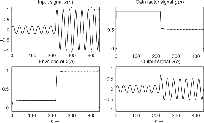
An example of a dynamic range controller's impact on a signal is shown in Figure 4.8. In this example, the dynamic range controller is a compressor: during periods of low signal level (first half of the shown input signal x(n)), the gain g(n) is set to 1, while for higher input levels (second half), the gain is decreased to reduce the signal's amplitude. Thus the difference in signal levels along time is reduced, compressing the signal's dynamic range.

Figure 4.8 The input signal x(n), the envelope of x(n), the derived gain factor g(n) and the output signal y(n).

Signal Processing

The level detector follows one of the approaches described in Section 4.3. Two commonly used choices are:

• A full-wave rectifier in combination with an AR-averager (see Figure 4.9) with very short attack time may be used to track the peak value of the signal.
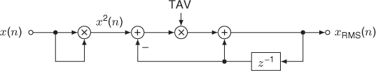
• A squarer averaged with only a single time-constant (see Figure 4.10) provides the RMS value, measuring the signal's power.

Figure 4.9 Peak measurement (envelope detector/follower) for a dynamic range controller.

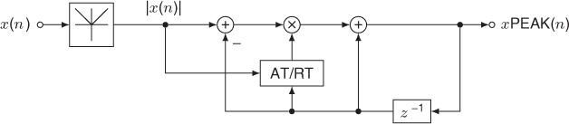
Figure 4.10 RMS measurement (envelope detector/follower) for a dynamic range controller [McN84, Zöl05].

Typical dynamic range controllers contain one of these level detectors, or even both, to be able to react to sudden level increases with the peak detector, while usually operating based on the RMS measurement.

The static curve decides which function (limiter, compressor, expander, …) the dynamic range controller assumes. It is best described on a dB scale, so we introduce X, G and Y for the levels of the respective signals in dB, i.e., X = 20 · log10(xPEAK(n)) or X = 10 · log10(xRMS(n)). The multiplication at the dynamic range controller's output then becomes Y = X + G.

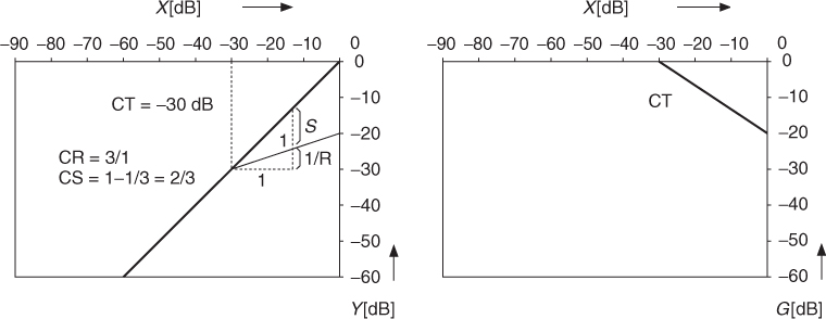
In this logarithmic domain, the gain is typically derived from the input level by a piecewise linear function. Figure 4.11 shows the characteristic curve of a typical compressor, mapping input to output level (on the left) and input level to gain (on the right). Up to a certain input level, the compressor threshold CT (−30 dB in this example), the gain is left at 0 dB. Above the threshold, the characteristic curve is defined by the ratio R, specifying the relation between input level change ΔX to output level change ΔY by . Alternatively, the slope factor may be specified instead of the ratio R.

Figure 4.11 Static characteristic: definition of slope S and ratio R [Zöl05] exemplified for a compressor.

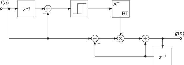
The dynamic behavior of a dynamic range controller is influenced by the level measurement approach (with attack AT and release time RT for peak measurement and averaging time TAV for RMS measurement) and further adjusted with a smoothing filter, as shown in Figure 4.12, which also employs special attack/release times. The calculation of the attack time parameter is carried out by

where tAT is the time parameter in seconds and T is the sampling period. The release time parameter RT and the averaging parameter TAV can be computed by the same formula by replacing tAT by tRT or tTAV, respectively. Further details and derivations can be found in [McN84, Zöl05]. The output of the static function is used as the input signal to the dynamic filter with attack and release times in Figure 4.12. The output signal g(n) is the gain factor for weighting the delayed input signal x(n − D) as shown in Figure 4.7. In the following sections some special dynamic range controllers are discussed in detail.

Figure 4.12 Dynamic filter: attack and release time adjustment for a dynamic range controller [McN84, Zöl05].

4.2.1 Limiter

The purpose of a limiter is to provide control over the highest peaks in the signal, but to otherwise change the dynamics of the signal as little as possible. This is achieved by employing a characteristic curve with an infinite ratio R = ∞ above a limiter threshold LT, i.e.,

4.8

Thus, the output level Y = X + G should never exceed the threshold LT. By lowering the peaks, the overall signal can be boosted. Beside limiting single instrument signals, limiting is also often performed on the final mix of a multichannel application.

A limiter makes use of peak level measurement and should react very quickly when the input signal exceeds the limiter threshold. Typical parameters for a limiter are tAT = 0.02…10 ms and tRT = 1…5000 ms, for both the peak measurement and the smoothing filter.

An actual implementation, like the one in Figure 4.13, may perform the gain computation in linear values by

4.9

where is the threshold on the linear scale. This approach is also used in M-file 4.1, a very simple limiter implementation with the same filter coefficients in the level detector and the smoothing filter. Figure 4.14 demonstrates the behavior of the time signals inside a limiter configuration of Figure 4.13.

Figure 4.13 Block diagram of a limiter.

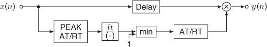
Figure 4.14 Signals for limiter.

4.2.2 Compressor and Expander

While a limiter completely eliminates any dynamics above a certain threshold by keeping the output level constant, a compressor only reduces the dynamics, compressing the dynamic range. The reduced dynamics can be exploited to increase the overall level, thereby boosting the loudness, without exceeding the allowed amplitude range. An expander does just the opposite of the compressor, increasing dynamics by mapping small level changes of the input to larger changes of the output level. Applying an expander to low-level signals gives a lively sound characteristic. The corresponding ratios and slopes of the characteristic curve are CR > 1 and 0 < CS < 1 for the compressor and 0 < ER < 1 and ES < 0 for the expander.

Compressors and expanders typically employ RMS level detectors with an averaging time in the range ms and a smoothing filter with tAT = 0.1 … 2600 ms and tRT = 1 … 5000 ms.

Combining a compressor for high signal levels with an expander for low signal levels leads to the gain computation

4.10

4.11

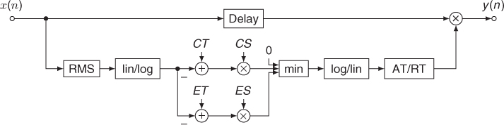
Here CT and ET denote the thresholds above which the compressor and below which the expander affect the signal, respectively. The resulting combined system is depicted in Figure 4.15. Again, the gain can alternatively be calculated without using logarithmic values by

4.12

where the square root operation of the RMS measurement is moved to the exponenents by halving the respective slopes. This approach makes conversion to and from the logarithmic domain unnecessary, but requires exponentiation. An implementation following the approach of Figure 4.15 is given in M-file 4.2.

Figure 4.15 Block diagram of a compressor/expander [Zöl05].

Parallel Compression

The usual application of compressors is the reduction of the amplitude variations above a specified threshold. In some circumstances however, e.g., for percussion instruments or an acoustic guitar, it is desired to leave unaffected the high-amplitude transients while enhancing the weaker parts of the signal. For such applications, parallel compression is recommended, where a heavily compressed version of the signal is added to the unaffected signal. The soft parts of the sound are heavily compressed using typically a low threshold, a high ratio and a short attack time. The compressed part is then amplified and mixed to the original signal. The resulting sound retains the transparency of the original sound because the transients are unaffected. This type of processing is sometimes referred to as New-York compression or side-chain compression [Bev77, Hul97, Kat07, Izh10].

Multiband Compression

Depending on the spectral content of the sound to process, compression might be required only on a selected frequency band. Let us consider the musical example of a piece for tuba and live electronics where the fingering and the breathing noises had to be processed irrespective of the overwhelming low frequency tones of the instrument. The solution was the insertion of a high-pass filter in the main path as well as the side-chain of a compressor so that the device left the lower part of the spectrum unaffected by the compression.

For the general case where several frequency bands of the spectrum have to be processed individually, the multiband compressor has been developed. A filter bank splits the input signal in several bands (usually three to five) which are then individually processed. The side-chain signal of each compressor is also derived from a band-limited version of the input signal. The filter-bank for the side-chain is usually the same as the for the input signal, but it is sometimes implemented as an independent processing unit so that intricate relations can be set up where the content of the input signal in a limited frequency band drives the compression in another frequency band.

Multiband dynamics processors are often used during mastering. At this stage, no direct correction of the individual musical parts is possible since the mix is finished and the music is usually available as a stereo track. Under the assumption that each musical part or instrument mainly occupies a particular frequency band, minor corrections are still possible if they are band limited.

One advantage of multiband compression is that the unwanted side-effects of compression, such as alteration of the tonal balance or distortions, can be limited to a given frequency band. With the objective of dynamic range compression, the reduction of the ratio of peak to RMS amplitude can be more effectively implemented in individual frequency bands than at the full audio bandwidth. This allows the increase of the overall loudness of the track. Considering that the casual listener often gives preference to the louder of two musical works, a trend has developed towards always higher average levels. Moderation is, however, necessary because the “loudness war” can induce severe degradations of the audio and musical quality [Kat07, Lun07].

4.2.3 Noise Gate

A noise gate can be considered as an extreme expander with a slope of −∞. This results in the complete muting of signals below the chosen threshold NT. As the name implies, the noise gate is typically used to gate out noise by setting the threshold just above the level of the background noise, such that the gate only opens when a desired signal with a level above the threshold is present. A particular application is found when recording a drum set. Each element of the drum set has a different decay time. When they are not manually damped, their sounds mix together and the result is no longer distinguishable. When each element is processed by a noise gate, every sound can automatically be faded out after the attack part of the sound. This results in an overall cleaner sound.

The functional units of a noise gate are shown in Figure 4.16. The decision to activate the gate is typically based on a peak measurement which leads to a fade in/fade out of the gain factor g(n) with appropriate attack and release times. Further possible refinements include the use of two thresholds to realize a hysteresis and a hold time to avoid unpleasant effects when the input level fluctuates around the threshold. These are demonstrated in the implementation given in M-file 4.3 [Ben97].

Figure 4.16 Block diagram of a noise gate [Zöl05].

Further implementations of limiters, compressors, expanders and noise gates can be found in [Orf96] and in [Zöl05], where special combined dynamic range controllers are also discussed.

4.2.4 De-esser

A de-esser is a signal processing device for processing speech and vocals. It consists of a bandpass filter tuned to the frequency range between 2 and 6 kHz to detect the level of the signal in this frequency band. If a certain threshold is exceeded, the gain factor of a peak or notch filter tuned to the same frequency band is controlled to realize a compressor for that band only, as shown in Figure 4.17. De-essers are mainly applied to speech or vocal signals to avoid high frequency sibilance.

Figure 4.17 Block diagram of a de-esser.

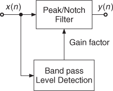
As an alternative to the bandpass/notch filters, highpass and shelving filters are used with good results. In order to make the de-esser more robust against input level changes, the threshold should depend on the overall level of the signal—that is, a relative threshold [Nie00].

4.2.5 Infinite Limiters

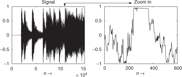
In order to catch overshoots from a compressor and limiter, a clipper or infinite limiter may be used [Nie00]. In contrast to the previously considered dynamic range controllers, the infinite limiter is a nonlinear operation working directly on the waveform by flattening the signal above a threshold. The simplest one is hard clipping, which generates lots of high-order harmonics. A gentler infinite limiter is the soft clipper, which rounds the signal shape before the absolute clipping threshold. Although infinite limiting should usually be avoided during mix down of multi channel recordings and recording sessions, several CDs make use of infinite limiting or saturation (see wave file in Figure 4.18 and listen to Carlos Santana/Smooth [m-San99]). A more detailed description of clipping effects and their artistic use is given in the following section.

Figure 4.18 Infinite limiting (Santana—“Smooth”).