5.5 Spatial Audio Effects for Multichannel Loudspeaker Layouts

5.5.1 Loudspeaker Layouts

In the history of multichannel audio [Ste96, Dav03, Tor98] multiple different loudspeaker layouts with more than two loudspeakers have been specified. The most frequently used layouts are presented in this chapter. In the 1970s, the quadraphonic setup was proposed, in which four loudspeakers are placed evenly around the listener at azimuth angles ±45° and ±135°. This layout was never successful because of problems related to reproduction techniques of that time, and because the layout itself had too few loudspeakers to provide good spatial quality in all directions around the listener [Rum01].

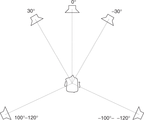
For cinema sound, a system was evolved in which the frontal image stability of the standard stereophonic setup was enhanced by one extra center channel, and two surround channels were used to create atmospheric effects and room perception. This kind of setup was first used in Dolby's surround sound system for cinemas from 1976 [Dav03]. Later, the layout was investigated [The91], and ITU gave a recommendation about the layout in 1992 [BS.94]. In the late 1990s, this layout also became common in domestic use. It is widely referred to as the 5.1 system, where 5 stands for the number of loudspeakers, and .1 stands for the low-frequency channel. In the recommendation, three frontal loudspeakers are at directions 0° and ±30°, and two surround channels at , as shown in Figure 5.5. The system has been criticized for not delivering good directional quality anywhere but in front [Rum01]. To achieve better quality, it can be extended by adding loudspeakers. Layouts with 6–12 loudspeakers have been proposed, and are presented in [Rum01].

Figure 5.5 Five channel surround loudspeaker layout based on ITU recommendation BS775.1.

In computer music, media installations and in academic projects, loudspeaker setups, in which the loudspeakers have equal spacing, have been used. In horizontal arrays the number of loudspeakers can be, for example, six (hexagonal array) or eight (octagonal array). In wave-field synthesis, see Section 5.5.6, the number of loudspeakers is typically between 20 and 200. In theaters and in virtual environment systems there exist systems in which loudspeakers are also placed above and/or below the listener.

5.5.2 2-D Loudspeaker Setups

In 2-D loudspeaker setups all loudspeakers are on the horizontal plane. Pair-wise amplitude panning [Cho71] is the best method to position virtual sources with such setups, when the number of loudspeakers is less than about 20. In pair-wise panning the sound signal is applied only to two adjacent loudspeakers of the loudspeaker setup at one time. The pair between which the panning direction lies is selected. Different formulations for pair-wise panning are Chowning's law [Cho71], which is not based on any psychoacoustic criteria, or 2-D vector-base amplitude panning (VBAP) [Pul97], which is a generalization of the tangent law (Equation (5.2)) for stereophonic panning.

In VBAP a loudspeaker pair is specified with two vectors. The unit-length vectors lm and ln point from the listening position to the loudspeakers. The intended direction of the virtual source (panning direction) is presented with a unit-length vector p. Vector p is expressed as a linear weighted sum of the loudspeaker vectors

5.12

Here gm and gn are the gain factors of the respective loudspeakers. The gain factors can be solved as

5.13

where and . The calculated factors are used in amplitude panning as gain factors of the signals applied to respective loudspeakers after suitable normalization, e.g., ||g|| = 1.

The directional quality achieved with pair-wise panning was studied in [Pul01]. When the loudspeakers are symmetrically placed on the left and right of the listener, VBAP estimates the perceived angle accurately. When the loudspeaker pair is not symmetrical with the median plane, the perceived direction is biased towards the median plane [Pul01], which can be more or less compensated [Pul02].

When there is a loudspeaker in the panning direction, the virtual source is sharp, but when panned between loudspeakers, the binaural cues are unnatural to some degree. This means that the directional perception of the virtual source varies with panning direction, which can be compensated by always applying sound to more than one loudspeaker [Pul99, SK04]. As in pair-wise panning, outside the best listening position the perceived direction collapses to the nearest loudspeaker producing a specific sound. This implies that the maximal directional error is of the same order of magnitude with the angular separation of loudspeakers from the listener's viewpoint in pair-wise panning. In practice, when the number of loudspeakers exceeds about eight, the virtual sources are perceived to be in the similar directions in a large listening area.

A basic implementation of 2-D VBAP is included here as a MATLAB function.

5.5.3 3-D Loudspeaker Setups

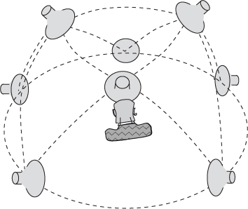
A 3-D loudspeaker setup denotes here a setup in which all loudspeakers are not in the same plane as the listener. Typically this means that there are some elevated and/or lowered loudspeakers added to a horizontal loudspeaker setup. Triplet-wise panning can be used in such setups [Pul97]. In it, a sound signal is applied to a maximum of three loudspeakers at one time that form a triangle from the listener's viewpoint. If more than three loudspeakers are available, the setup is divided into triangles, one of which is used in the panning of a single virtual source at one time, as shown in Figure 5.6. 3-D vector-base amplitude panning (3-D VBAP) is a method to formulate such setups [Pul97]. It is formulated in an equivalent way to pair-wise panning in the previous section. However, the number of gain factors and loudspeakers is naturally three in the equations. The angle between the median plane and virtual source is estimated correctly with VBAP in most cases, as in pair-wise panning. However, the perceived elevation of a sound source is individual to each subject [Pul01].

Figure 5.6 A 3-D triangulated loudspeaker system for triplet-wise panning.

A basic implementation of 3-D VBAP for the loudspeaker setup in Figure 5.6 is shown here as a MATLAB function.

5.5.4 Coincident Microphone Techniques and Ambisonics

In coincident microphone technologies first- or higher-order microphones positioned ideally in the same position are used to capture sound for multichannel playback. The ambisonics technique [Ger73, ED08] is a form of this. The most common microphone for these applications is the first-order four-capsule B-format microphone, producing a signal w(t) with omnidirectional characteristics, which has been scaled down by . The B-format microphone also outputs three signals x(t), y(t), and z(t) with figure-of-eight characteristics pointing to corresponding Cartesian directions. The microphones are ideally in the same position. Higher-order microphones have also been proposed and are commercially available, which have much more capsules than the first-order microphones.

In most cases, the microphones are of first order. When the loudspeaker signals are created from the recorded signal, the channels are simply added together with different gains. Thus each loudspeaker signal can be considered as a virtual microphone signal having first-order directional characteristics. This is expressed as

5.14

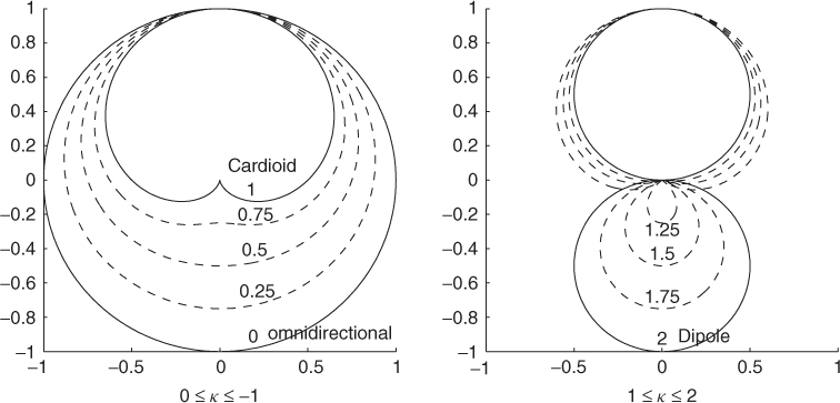
where s(t) is the produced virtual microphone signal having an orientation of azimuth θ and elevation ϕ. The parameter κ ∈ [0, 2] defines the directional characteristics of the virtual microphone from omnidirectional to cardioid and dipole, as shown in Figure 5.7.

Figure 5.7 The directional pattern of virtual microphones which can be generated from first-order B-format recordings. Figure reprinted with permission from [Vil08].

In multichannel reproduction of such first-order B-format recordings, a virtual microphone signal is computed for each loudspeaker. In practice such methods provide good quality only in certain loudspeaker configurations [Sol08] and at frequencies well below 1 kHz. At higher frequencies the high coherence between the loudspeaker signals, which is caused by the broad directional patterns of the microphones, leads to undesired effects such as coloration and loss of spaciousness. Using higher-order microphones these problems are less severe, though some problems with microphone self-noise may appear.

The decoding of first-order B-format microphone signals to a horizontal loudspeaker layout with directional characteristics controllable by κ is shown in the following example:

The previous example was of reproducing a recorded sound scenario. Such coincident recording can also be simulated to perform synthesis of spatial audio [MM95] for 2-D or 3-D loudspeaker setups. In this case it is an amplitude-panning method in which a sound signal is applied to all loudspeakers placed evenly around the listener with gain factors

5.15

where gi is the gain of ith speaker, N is the number of loudspeakers, α is the angle between loudspeaker and panning direction, cos(mαi) represents a single spherical harmonic with order m, M is the order of Ambisonics, and pm are the gains for each spherical harmonic [DNM03, Mon00]. When the order is low, the sound signal emanates from all the loudspeakers, which causes some spatial artifacts due to unnatural behavior of binaural cues [PH05]. In such cases, when listening outside the best listening position, the sound is also perceived at the nearest loudspeaker which produces the sound. This effect is more prominent with first-order ambisonics than with pair- or triplet-wise panning, since in ambisonics virtually all loudspeakers produce the same sound signal. The sound is also colored, for the same reason, i.e., multiple propagation paths of the same signal to ears produce comb-filter effects. Conventional microphones can be used to realize first-order ambisonics.

When the order is increased, the cross-talk between loudspeakers can be minimized by optimizing gains of spherical harmonics for each loudspeaker in a listening setup [Cra03]. Using higher-order spatial harmonics increases both directional and timbral virtual source quality, since the loudspeaker signals are less coherent. The physical wave field reconstruction is then more accurate, and different curvatures of wavefronts, as well as planar wavefronts can be produced [DNM03], if a large enough number of loudspeakers is in use. The selection of the coefficients for different spherical harmonics has to be done carefully for each loudspeaker layout.

A simple implementation of computing second-order ambisonic gains for a hexagonal loudspeaker layout is shown here:

5.5.5 Synthesizing the Width of Virtual Sources

A loudspeaker layout having loudspeakers around the listener can also be used to control the width of the sound source, or even to produce an enveloping perception of the sound source. A simple demonstration can be made by playing back pink noise with all loudspeakers, where the noises are independent of each other [Bla97]. The sound source is then perceived to surround the listener totally.

The precise control of the width of the virtual source is a complicated topic. However, simple and effective spatial effects can be performed by using some of the loudspeakers to generate a wide virtual source. The example of decorrelating a monophonic input signal for stereophonic listening shown in Section 5.3.2 can be also used with multichannel loudspeaker setups. In such cases, the number of columns in the noise matrix corresponds to the number of loudspeakers to which the decorrelated sound is applied, and the convolution has to be computed for each loudspeaker channel. The virtual source will be more or less perceived to originate evenly from the loudspeakers and from the space between them. Unfortunately, the drawback of time-smearing of transients is also present in this case.

Note that this is a different effect than the effect generated with reverberators, which are discussed in Section 5.6, although the processing is very similar. The reverberators simulate the room effect, and try to create the perception of a surrounding reverberant tail, and in contrast the effect discussed in this section generates the perception of a surrounding non-reverberant sound. However, such effects cannot be achieved with all types of signals, due to human perceptual capabilities, as discussed briefly in Section 5.2.3.

5.5.6 Time Delay-based Systems

There are a number of methods proposed, which instead of using amplitude differences use time-delays in positioning the virtual sources. The most complete one, the wave field synthesis is presented first, after which Moore's room-inside-room approach is discussed.

Wave-field synthesis is a technique that requires a large number of carefully equalized loudspeakers [BVV93, VB99]. It aims to reconstruct the whole sound field in a listening room. When a virtual source is reproduced, the sound for each loudspeaker is delayed and amplified in a manner that a desired circular or planar sound wave occurs as a superposition of sounds from each loudspeaker. The virtual source can be positioned far behind the loudspeakers, or in some cases even in the space inside the loudspeaker array, as shown in Figure 5.8. The loudspeaker signals have to be equalized depending on virtual source position [ARB04].

Figure 5.8 Wave-field synthesis concept. A desired 2-D sound field can be constructed using a large loudspeaker array. Figure reprinted with IEEE permission from [VB99].

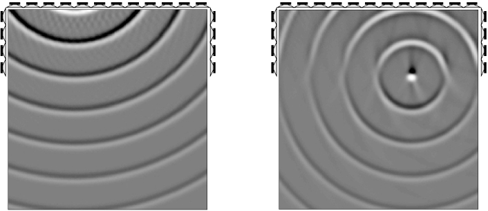
Theoretically the wave-field synthesis is superior as a technique, as the perceived position of the sound source is correct within a very large listening area. Unfortunately, to create a desired wave field in the total area inside the array, it demands that the loudspeakers are at a distance of maximally a half wavelength from each other. The area in which a perfect sound field synthesis is achieved shrinks with increasing frequency [DNM03]. In practice, due to the perception mechanisms of humans, more error can be allowed above approximately 1.5 kHz. Arrays for wave-field synthesis have been built for room acoustics control and enhancement to be used in theaters and multipurpose auditoria [VB99].

Time delays also can be used when creating spatial effects with loudspeaker setups with fewer loudspeakers than used in wave-field synthesis. The use of time delays for positioning virtual sources was considered for a two-channel stereophonic layout in Section 5.3.2. It was noted that short delays of a few milliseconds make the virtual sources perceived as spatially spread. This effect of course also applies with multi-loudspeaker setups. With longer delays, the precedence effect makes the sound direction perceived to be form the loudspeaker where the sound arrived first. This technique has also been used for multichannel loudspeaker layouts, as in Moore's approach, where the relative time delay between the loudspeaker feeds is controlled. A model supporting this approach was introduced by Moore [Moo83], and can be described as a physical and geometric model. The metaphor underlying the Moore model is that of a room-within-a-room, where the inner room has holes in the walls, corresponding to the positions of the loudspeakers, and the outer room is the virtual room where the sound events take place. When a single virtual source is applied in the virtual world, all the loudspeakers emanate the same sound with different amplitudes and delays. This is a similar idea to wave-field synthesis, though the mathematical basis is less profound, and the number of loudspeakers utilized is typically smaller. The recreated sound field will be limited to low frequencies, and at higher frequencies comb-filter effects and unstable directions for virtual sources will appear. However, if the delays are large enough, the virtual source will be perceived at all listening positions to the loudspeaker which emanates the sound first. The effects introduced by the Moore model are directly related with the artifacts one would get when listening to the outside world through windows.

5.5.7 Time-frequency Processing of Spatial Audio

The directional resolution of spatial hearing is limited within auditory frequency bands [Bla97]. In principle, all sound within one critical band can be only perceived as a single source with broader or narrower extent. In some special cases a binaural narrow-band sound stimulus can be perceived as two distinct auditory objects, but the perception of three or more concurrent sources is generally not possible. This is different from visual perception, where already one eye can detect the directions of a large number of visual objects sharing the same color.

The limitations of spatial auditory perception imply that the spatial realism needed in visual reproduction is not needed in audio. In other words, the spatial accuracy in reproduction of acoustical wave field can be compromised without decrease in perceptual quality. There are some recent technologies which exploit this assumption. Methods to compress multichannel audio files to 1–2 audio signals with metadata have been proposed [BF08, GJ06], where the level and time differences between the channels are analyzed in the time-frequency domain, and are coded as metadata to the signal. A related technology for spatial audio, directional audio coding (DirAC) [Pul07], is a signal-processing method for spatial sound, which can be applied to spatial sound reproduction for any multichannel loudspeaker layout, or for headphones. The other applications suggested for it include teleconferencing and perceptual audio coding.

In DirAC, it is assumed that at one time instant and at one critical band the spatial resolution of auditory system is limited to decoding one cue for direction and another for inter-aural coherence. It is further assumed that if the direction and diffuseness of sound field is measured and reproduced correctly, a human listener will perceive the directional and coherence cues correctly.

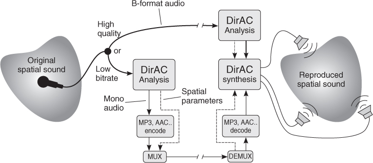
The concept of DirAC is illustrated in Figure 5.9. In the analysis phase, the direction and diffuseness of the sound field is estimated in auditory frequency bands depending on time, forming the metadata transmitted together with a few audio channels. In the “low-bitrate” approach shown in the figure, only one channel of audio is transmitted. The audio channel may also be further compressed to obtain a lower transmission data rate. The version with more channels is shown as a “high-quality version,” where the number of transmitted channels is three for horizontal reproduction, and four for 3-D reproduction. In the high-quality version the analysis may be conducted at the receiving end. It has been proven that the high-quality version of DirAC produces better perceptual quality in loudspeaker listening than other available techniques using the same microphone input [VLP09].

Figure 5.9 Two typical approaches of DirAC: High quality (top) and low bitrate (bottom). Figure reprinted with AES permission from [Vil08].

The processing in DirAC and in other time-frequency-domain processing for spatial audio is typically organized as an analysis-transmission-synthesis chain. To give an idea of the analysis process, the analysis part of DirAC is now discussed in detail, followed by a code example.

The aim of directional analysis, which is shown in Figure 5.10, is to estimate at each frequency band the direction of arrival of sound, together with an estimate of if the sound is arriving from one or multiple directions at the same time. In principle this can be performed with a number of techniques, however, an energetic analysis of the sound field has been found to be suitable, which is shown in Figure 5.10. The energetic analysis can be performed when the pressure signal and velocity signals in one, two or three dimensions are captured from a single position.

Figure 5.10 DirAC analysis. Figure reprinted with AES permission from [Vil08].

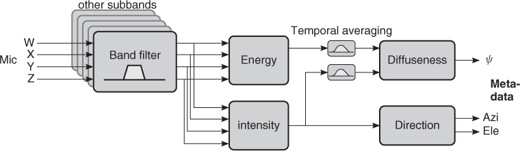
The first-order B-format signals described in Section 5.5.4 can be used for directional analysis. The sound pressure can be estimated using the omnidirectional signal w(t) as , expressed in the STFT domain. The figure-of-eight signals x(t), y(t), and z(t) are grouped in the STFT domain into a vector U = [X, Y, Z], which estimates the 3-D sound field velocity vector. The energy E of sound field can be computed as

5.16

where ρ0 is the mean density of air, and c is the speed of sound. The capturing of B-format signals can be obtained with either coincident positioning of directional microphones, or with closely spaced set of omnidirectional microphones. In some applications, the microphone signals may be formed in the computational domain, i.e., simulated. The analysis is repeated as frequently as is needed for the application, typically with an update frequency of 100–1000 Hz.

The intensity vector I expresses the net flow of sound energy as a 3-D vector, and can be computed as

5.17

where denotes complex conjugation. The direction of sound is defined as the opposite direction to the intensity vector at each frequency band. The direction is denoted as the corresponding angular azimuth and elevation values in the transmitted metadata. The diffuseness of the sound field is computed as

5.18

where E is the expectation operator. Typically the expectation operator is implemented with temporal integration, as in the example below. This process is also called “smoothing.” The outcome of this equation is a real-valued number between zero and one, characterizing whether the sound energy is arriving from a single direction, or from all directions.

An example of directional analysis of B-format signals is presented in the following. The synthesis of sound is not shown here, however the reader is encouraged to use the analysis results to build different spatial effects of his own.