5.7 Modeling of Room Acoustics

The room effect, i.e., the room impulse response, can be created by modeling how sound propagates and reflects from surfaces if the geometry of a room is available. Such a process is called room acoustics modeling and several techniques are discussed in Section 5.7.4. In many cases the geometry of a room is not needed since an artificial room impulse response can be created from a perceptual point of view. In fact, the human hearing is not very sensitive to details in the reverberant tail and any decaying response can be used as an effect.

Even if we have enough computer power to compute convolutions by long impulse responses in real time, there are still reasons to prefer reverberation algorithms based on feedback delay networks in many practical contexts. The reasons are similar to those that make a CAD description of a scene preferable to a still picture whenever several views have to be extracted or the environment has to be modified interactively. In fact, it is not easy to modify a room impulse response to reflect some of the room attributes, e.g., its high-frequency absorption. If the impulse response is coming from a room acoustics modeling algorithm, these manipulations can be operated at the level of room description, and the coefficients of the room impulse response are transmitted to the real-time convolver. In low-latency block-based implementations, we can even have faster update rates for the smaller early chunks of the impulse response, and slower update rates for the reverberant tail. Still, continuous variations of the room impulse response are easier to render using a model of reverberation operating on a sample-by-sample basis. For this purpose dozens of reverberation algorithms have been developed and in the following some of them are introduced in more detail.

5.7.1 Classic Reverb Tools

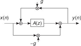
In the second half of the twentieth century, several engineers and acousticians tried to invent electronic devices capable of simulating the long-term effects of sound propagation in enclosures. The most important pioneering work in the field of artificial reverberation has been that of Manfred Schroeder at the Bell Laboratories in the early sixties [Sch61, Sch62, Sch70, Sch73, SL61]. Schroeder introduced the recursive comb filters and the delay-based allpass filters as computational structures suitable for the inexpensive simulation of complex patterns of echoes. In particular, the allpass filter based on the recursive delay line has the form

5.19

where m is the length of the delay in samples. The filter structure is depicted in Figure 5.13, where A(z) is usually replaced by a delay line. This filter allows one to obtain a dense impulse response and a flat frequency response. Such a structure became rapidly a standard component used in almost all the artificial reverberators designed up to now [Moo79]. It is usually assumed that the allpass filters do not introduce coloration in the input sound. However, this assumption is valid from a perceptual viewpoint only if the delay line is much shorter than the integration time of the ear, i.e., about 50 ms [ZF90]. If this is not the case, the time-domain effects become much more relevant and the timbre of the incoming signal is significantly affected.

Figure 5.13 The allpass filter structure.

In the seventies, Michael Gerzon generalized the single-input single-output allpass filter to a multi-input multi-output structure, where the delay line of m samples has been replaced by an order-N unitary network [Ger76]. Examples of trivial unitary networks are orthogonal matrices, and parallel connections of delay lines or allpass filters. The idea behind this generalization is that of increasing the complexity of the impulse response without introducing appreciable coloration in frequency. According to Gerzon's generalization, allpass filters can be nested within allpass structures, in a telescopic fashion. Such embedding is shown to be equivalent to lattice allpass structures [Gar97b], and it is realizable as long as there is at least one delay element in the block A(z) of Figure 5.13. An example MATLAB code with a delay of 40 samples is:

Extensive experimentation on structures for artificial reverberation was conducted by Moorer in the late seventies [Moo79]. He extended the work done by Schroeder [Sch70] in relating some basic computational structures (e.g., tapped delay lines, comb and allpass filters) with the physical behavior of actual rooms. In particular, it was noticed that the early reflections have great importance in the perception of the acoustic space, and that a direct-form FIR filter can reproduce these early reflections explicitly and accurately. Usually this FIR filter is implemented as a tapped delay line, i.e., a delay line with multiple reading points that are weighted and summed together to provide a single output. This output signal feeds, in Moorer's architecture, a series of allpass filters and parallel comb filters. Another improvement introduced by Moorer was the replacement of the simple gain of feedback delay lines in comb filters with lowpass filters resembling the effects of air absorption and lossy reflections.

An original approach to reverberation was taken by Julius Smith in 1985, when he proposed digital waveguide networks (DWNs) as a viable starting point for the design of numerical reverberators [Smi85]. The idea of waveguide reverberators is that of building a network of waveguide branches (i.e., bidirectional delay lines simulating wave propagation in a duct or a string) capable of producing the desired early reflections and a diffuse, sufficiently dense reverb. If the network is augmented with lowpass filters it is possible to shape the decay time with frequency. In other words, waveguide reverberators are built in two steps: the first step is the construction of a prototype lossless network, the second step is the introduction of the desired amount of losses. This procedure ensures good numerical properties and good control over stability [Smi86, Vai93]. In ideal terms, the quality of a prototype lossless reverberator is evaluated with respect to the whiteness and smoothness of the noise that is generated in response to an impulse. The fine control of decay time at different frequencies is decoupled from the structural aspects of the reverberator.

Among the classic reverberation tools we should also mention the structures proposed by Stautner and Puckette [SP82], and by Jot [Jot92]. These structures form the basis of feedback delay networks, which are discussed in detail in Section 5.7.2.

Clusters of Comb/allpass Filters

The construction of high-quality reverberators is half an art and half a science. Several structures and many parameterizations have been proposed in the past, especially in non-disclosed form within commercial reverb units [Dat97]. In most cases, the various structures are combinations of comb and allpass elementary blocks, as suggested by Schroeder in the early work. As an example, we briefly describe Moorer's preferred structure [Moo79], depicted in Figure 5.14. The block (a) of Moorer's reverb takes care of the early reflections by means of a tapped delay line. The resulting signal is forwarded to the block (b), which is the parallel of a direct path on one branch, and a delayed, attenuated diffuse reverberator on the other branch. The output of the reverberator is delayed in such a way that the last of the early echoes coming out of block (a) reaches the output before the first of the non-null samples coming out of the diffuse reverberator. In Moorer's preferred implementation, the reverberator of block (b) is best implemented as a parallel of six comb filters, each with a first-order lowpass filter in the loop, and a single allpass filter. In [Moo79], it is suggested to set the allpass delay length to 6 ms and the allpass coefficient to 0.7. Despite the fact that any allpass filter does not add coloration in the magnitude frequency response, its time response can give a metallic character to the sound, or add some unwanted roughness and granularity. The feedback attenuation coefficients and the lowpass filters of the comb filters can be tuned to resemble a realistic and smooth decay. In particular, the attenuation coefficients gi determine the overall decay time of the series of echoes generated by each comb filter. If the desired decay time (usually defined for an attenuation level of 60 dB) is Td, the gain of each comb filter has to be set to

5.20

where Fs is the sample rate and mi is the delay length in the samples. Further attenuation at high frequencies is provided by the feedback lowpass filters, whose coefficient can also be related to decay time at a specific frequency or fine tuned by direct experimentation. In [Moo79], an example set of feedback attenuation and allpass coefficients is provided, together with some suggested values of the delay lengths of the comb filters. As a general rule, they should be distributed over a ratio 1:1.5 between 50 and 80 ms. Schroeder suggested a number-theoretic criterion for a more precise choice of the delay lengths [Sch73]: the lengths in samples should be mutually coprime (or incommensurate) to reduce the superimposition of echoes in the impulse response, thus reducing the so-called flutter echoes. This same criterion might be applied to the distances between each echo and the direct sound in early reflections. However, as was noticed by Moorer [Moo79], the results are usually better if the taps are positioned according to the reflections computed by means of some geometric modeling technique, such as the image method. As is explained next, even the lengths of the recirculating delays can be computed from the geometric analysis of the normal modes of actual room shapes.

Figure 5.14 Moorer's reverberator.

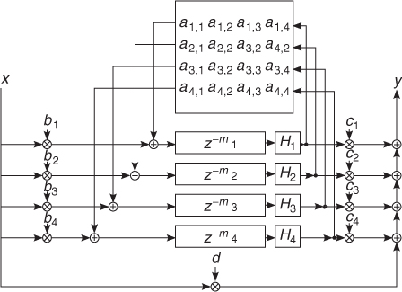
5.7.2 Feedback Delay Networks

In 1982, J. Stautner and M. Puckette [SP82] introduced a structure for artificial reverberation based on delay lines interconnected in a feedback loop by means of a matrix (see Figure 5.15). Later, structures such as this have been called feedback delay networks (FDNs). The Stautner–Puckette FDN was obtained as a vector generalization of the recursive comb filter

5.21

where the m-sample delay line was replaced by a bunch of delay lines of different lengths, and the feedback gain g was replaced by a feedback matrix G. Stautner and Puckette proposed the following feedback matrix:

5.22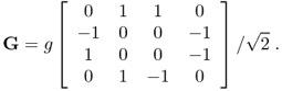

Due to its sparse special structure, G requires only one multiple per output channel.

Figure 5.15 Fourth-order feedback delay network.

An example of FDN without lowpass filters Hn is:

More recently, Jean-Marc Jot has investigated the possibilities of FDNs very thoroughly. He proposed to use some classes of unitary matrices allowing efficient implementation. Moreover, he showed how to control the positions of the poles of the structure in order to impose a desired decay time at various frequencies [Jot92]. His considerations were driven by perceptual criteria and the general goal was to obtain an ideal diffuse reverb. In this context, Jot introduced the important design criterion that all the modes of a frequency neighborhood should decay at the same rate, in order to avoid the persistence of isolated, ringing resonances in the tail of the reverb [JC91]. This is not what happens in real rooms though, where different modes of close resonance frequencies can be differently affected by wall absorption [Mor91]. However, it is generally believed that the slow variation of decay rates with frequency produces smooth and pleasant impulse responses.

General Structure

Referring to Figure 5.15, an FDN is built starting from N delay lines, each being τi = miTs seconds long, where Ts = 1/Fs is the sampling interval. The FDN is completely described by the following equations:

5.23

where , are the delay outputs at the nth time sample. If mi = 1 for every i, we obtain the well-known state space description of a discrete-time linear system [Kai80]. In the case of FDNs, mi are typically numbers on the orders of hundreds or thousands, and the variables si(n) are only a small subset of the system state at time n, being the whole state represented by the content of all the delay lines.

From the state-variable description of the FDN it is possible to find the system transfer function [Roc96, RS97] as

5.24

The diagonal matrix is called the delay matrix, and A = [ai, j]N×N is called the feedback matrix.

The stability properties of a FDN are all ascribed to the feedback matrix. The fact that ||A||n decays exponentially with n ensures that the whole structure is stable [Roc96, RS97].

The poles of the FDN are found as the solutions of

5.25

In order to have all the poles on the unit circle it is sufficient to choose a unitary matrix. This choice leads to the construction of a lossless prototype, but this is not the only choice allowed.

The zeros of the transfer function can also be found [Roc96, RS97] as the solutions of

5.26

In practice, once we have constructed a lossless FDN prototype, we must insert attenuation coefficients and filters in the feedback loop. For instance, following the indications of Jot [JC91], we can cascade every delay line with a gain

5.27

This corresponds to replacing D(z) with D(z/α) in (5.24). With this choice of the attenuation coefficients, all the poles are contracted by the same factor α. As a consequence, all the modes decay with the same rate, and the reverberation time (defined for a level attenuation of ) is given by

5.28

In order to have a faster decay at higher frequencies, as happens in real enclosures, we must cascade the delay lines with lowpass filters. If the attenuation coefficients gi are replaced by lowpass filters, we can still get a local smoothness of decay times at various frequencies by satisfying the condition (5.27), where gi and α have been made frequency dependent:

5.29

where A(z) can be interpreted as per-sample filtering [JSer, JC91, Smi92].

It is important to notice that a uniform decay of neighbouring modes, even though commonly desired in artificial reverberation, is not found in real enclosures. The normal modes of a room are associated with stationary waves, whose absorption depends on the spatial directions taken by these waves. For instance, in a rectangular enclosure, axial waves are absorbed less than oblique waves [Mor91]. Therefore, neighboring modes associated with different directions can have different reverberation times. Actually, for commonly found rooms having irregularities in the geometry and in the materials, the response is close to that of a room having diffusive walls, where the energy rapidly spreads among the different modes. In these cases, we can find that the decay time is quite uniform among the modes [Kut95].

Parameterization

The main questions arising after we established a computational structure called FDN are: What are the numbers that can be put in place of the many coefficients of the structure? How should these numbers be chosen?

The most delicate part of the structure is the feedback matrix. In fact, it governs the stability of the whole structure. In particular, it is desirable to start with a lossless prototype, i.e., a reference structure providing an endless, flat decay. The reader interested in general matrix classes that might work as prototypes is referred to the literature [Jot92, RS97, Roc97, Gar97b]. Here we only mention the class of circulant matrices, having the general form

5.30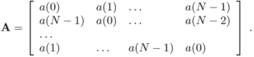

The stability of an FDN is related to the magnitude of its eigenvalues, which can be computed by the discrete Fourier transform of the first row, in the case of a circulant matrix. By keeping these eigenvalues on the unit circle (i.e., magnitude one) we ensure that the whole structure is stable and lossless. The control over the angle of the eigenvalues can be translated into a direct control over the degree of diffusion of the enclosure that is being simulated by the FDN. The limiting cases are the diagonal matrix, corresponding to perfectly reflecting walls, and the matrix whose rows are sequences of equal-magnitude numbers and (pseudo-)randomly distributed signs [Roc97].

Another critical set of parameters is given by the lengths of the delay lines. Several authors suggested to use lengths in samples that are mutually coprime numbers in order to minimize the collision of echoes in the impulse response. However, if the FDN is linked to a physical and geometrical interpretation, as it is done in the ball-within-a-box model [Roc95], the delay lengths are derived from the geometry of the room being simulated and the resulting digital reverb quality is related to the quality of the actual room. A delay line is associated with a harmonic series of normal modes, all obtainable from a plane-wave loop that bounces back and forth within the enclosure. The delay length for the particular series of normal modes is given by the time interval between two consecutive collisions of the plane wavefront along the main diagonal, i.e., twice the time taken to travel the distance

5.31

being f0 the fundamental frequency of the harmonic modal series.

5.7.3 Time-variant Reverberation

Reverberation algorithms are usually time invariant, meaning that the response does not change as a function of time. This is reasonable, since reverberation algorithms model an LTI system, an impulse response. However, in live performances and installations, it is sometimes beneficial to have a time-variant reverberation to prevent and reduce the coloration and instability due to the feedback caused by the proximity of microphones and loudspeakers. The frequency response of such a system is not ideally flat, which easily leads to acoustical feedback at the frequency with the highest loop gain. Several algorithms exist [NS99] to modify the frequency response of the system so that resonance frequencies vary over time.

One efficient implementation of time-variance to an FDN type reverberator has been proposed [LH01]. The FDN is modified to contain a comb-allpass filter at each delay line. The time variance is implemented by modulating the feedback coefficient of this comb-allpass filter with a few Hertz modulation frequency. Such modulations change the group delay of each delay line, resulting in the frequency shift of resonant frequencies. However, this shift is not constant at all frequencies and if all delay lines in the FDN have different modulation frequencies no audible pitch shift is perceived. Such an algorithm has been successfully applied in the creation of a physically small, but sonically large rehearsal space for a symphony orchestra [LPPS09].

5.7.4 Modeling Reverberation with a Room Geometry

In some applications, it is beneficial to have a room effect based on the defined room geometry. Then, the impulse response is created with computational room acoustics modeling methods. The methods can be divided into ray-based and wave-based methods, based on the underlying assumptions of the sound propagation [Sil10].

Wave-based Methods

Wave-based acoustic modeling aims to numerically solve the wave equation. Traditional techniques are the finite element (FEM) and the boundary element (BEM) methods [SK02]. However, these techniques are computationally too heavy for the whole audible frequency range, although at low frequencies they could be applied in combination with other techniques more suitable at higher frequencies. The digital waveguide mesh method is a newer wave-based technique, being computationally less expensive and thus more suitable for room impulse response creation or even for real-time auralization [MKMS07, Sav10]. A novel, very interesting wave-based method is the adaptive rectangular decomposition method [RNL09].

Ray-based Methods

In ray-based acoustic modeling sound is assumed to behave similarly to light. This approximation is valid at high frequencies, and makes it possible to utilize plenty of algorithms developed in computer graphics in the field of global illumination. All the ray-based methods are covered by the room acoustic rendering equation [SLKS07], and all methods can be seen as a special solution for this equation. The detailed presentation of the room acoustic rendering equation is outside the scope of this book, but the most common ray-based modeling methods are briefly introduced here.

The image-source method and beam-tracing methods are the most common techniques to find specular reflection paths. The image-source method [AB79, Bor84] is based on recursive reflection of sound sources against all the surfaces in the room. This results in a combinatory explosion, and in practice only low-order, i.e., early reflections can be found. Figure 5.16 illustrates the process by showing image sources up to fourth order in a very simple 2-D geometry. Beam-tracing methods, such as [FCE+98, LSLS09], are optimized versions for the same purpose capable of dealing with more complicated geometries and higher reflection orders. A related approach to beam tracing is frustum tracing [LCM07], which scales even better to very large models. For image-source computation with MATLAB see [CPB05]1 and [LJ08].2

Figure 5.16 Visualization of the image source method. The dots outside of the concert hall silhouette are the image sources. The response above is the energy response at the receiver position, which is on the balcony. Figures (a)–(d) contain first–fourth-order image sources, respectively.

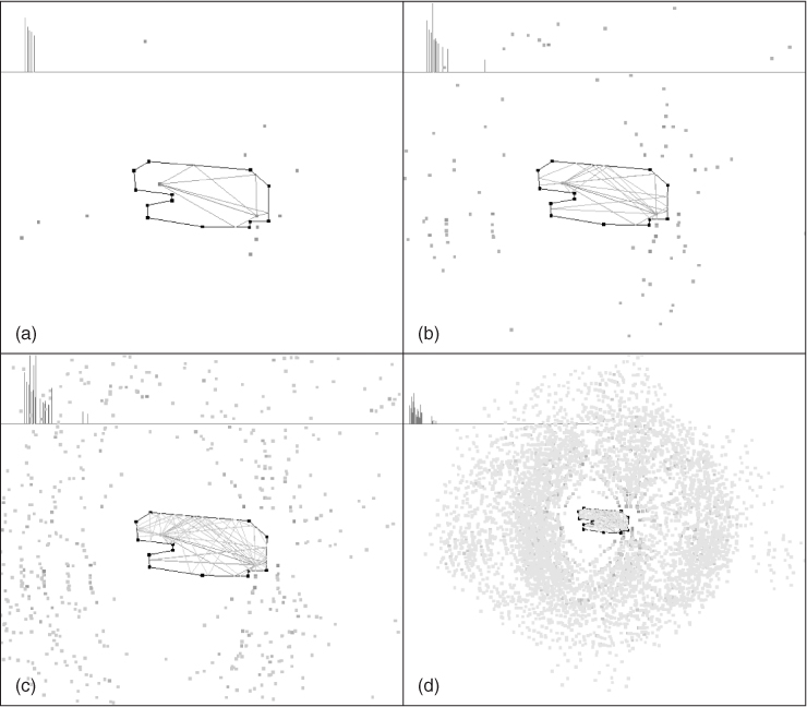
Ray tracing [KSS68] is the most popular offline algorithm for modeling sound propagation since it enables more advanced reflection modeling than the image-source method. A common approach is to shoot rays from the sound source in every direction, according to the directivity pattern of the source, and trace each ray until its energy level has decayed below a given threshold and at the same time keep track of instants when the ray hits a receiver, see Figures 5.17a and 5.17b.

Figure 5.17 The ray-tracing method produces (a) a sparse response. (b) If the receiver area is larger more reflections are modeled. (c) The acoustics radiance transfer method when the initial energy is distributed to the surface patches. (d) The whole response after 100 energy distributions.

The acoustic radiance transfer is a recently presented acoustic modeling technique based on progressive radiosity and arbitrary reflection models [SLKS07]. The acoustic energy is shot from the sound source to the surfaces of the model, which have been divided into patches, as illustrated in Figure 5.17c. Then, the propagation of the energy is followed from patch to patch and the intermediate results are stored on the patches. Finally, when the desired accuracy is achieved, the energy is collected from the patches to the listener.

These three methods have different properties for room-effect simulation. The image source method can only model specular reflections, but it is very efficient in finding perceptually relevant early reflections. As a reverberation effect the image source method is suitable for real-time processing, since the image sources, i.e., early reflections, can be spatially rendered and the late reverberation can be added with, for example, an FDN reverberator [SHLV99, LSH+02]. The ray-tracing method is not suitable for real-time reverberation processing. However, it is good at off line creation of the whole impulse response, which can be applied later with a real-time convolver. The acoustic radiance transfer method is the most advanced ray-based room acoustics modeling method, since it can handle both specular and diffuse reflections. Although the method is computationally extensive, the usage of the GPUs makes it possible to run the final gathering and sound rendering in real time, thus enabling interactive reverberation effects of environments with arbitrary reflection properties [SLS09].