
In this section we present and discuss a set of implementations of the different spectral models, building one implementation on top of another and making sure that each implementation is self-contained, thus being useful for some applications. Each implementation is an analysis/synthesis system that has as input a monophonic sound, ![]() , plus a set of parameters, and outputs a synthesized sound, y(n). If the parameters are set correctly and the input sound used is adequate for the model, the output sound should be quite close, from a perceptual point of view, to the input sound. We start with an implementation of the STFT, which should yield a mathematical input-ouput identity for any sound. On top of that we build an analysis/synthesis system based on detecting the spectral peaks, and we extend it to implement a simple sinusoidal model. The following system implements a sinusoidal model with a harmonic constraint, thus only working for pseudo-harmonic sounds. We then include the residual analysis, thus implementing a harmonic plus residual model. Finally we assume that the residual is stochastic and implement a harmonic plus stochastic residual model.
, plus a set of parameters, and outputs a synthesized sound, y(n). If the parameters are set correctly and the input sound used is adequate for the model, the output sound should be quite close, from a perceptual point of view, to the input sound. We start with an implementation of the STFT, which should yield a mathematical input-ouput identity for any sound. On top of that we build an analysis/synthesis system based on detecting the spectral peaks, and we extend it to implement a simple sinusoidal model. The following system implements a sinusoidal model with a harmonic constraint, thus only working for pseudo-harmonic sounds. We then include the residual analysis, thus implementing a harmonic plus residual model. Finally we assume that the residual is stochastic and implement a harmonic plus stochastic residual model.
10.3.1 Short-time Fourier Transform
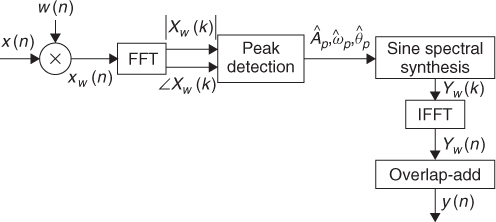
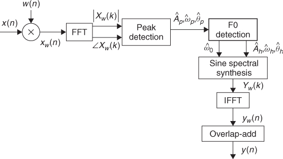
Figure 10.3 shows the general block diagram of an analysis/sysnthesis system based on the STFT.
Figure 10.3 Block diagram of an analysis/synthesis system based on the STFT.
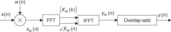
In order to use the STFT as a basis for the other spectral models we have to pay special attention to a number of issues related to the windowing process, specifically zero-phase windowing, the size and type of the analysis window, and the overlap-add process that is performed in the inverse transform process.
Below is the MATLAB code that implements a complete analysis/synthesis system based on the STFT.
M-file 10.1 (stft.m)
function y = stft(x, w, N, H)
% Authors: J. Bonada, X. Serra, X. Amatriain, A. Loscos
% Analysis/synthesis of a sound using the short-time Fourier transform
% x: input sound, w: analysis window (odd size), N: FFT size, H: hop size
% y: output sound
M = length(w); % analysis window size
N2 = N/2+1; % size of positive spectrum
soundlength = length(x); % length of input sound array
hM = (M-1)/2; % half analysis window size
pin = 1+hM; % initialize sound pointer in middle of analysis window
pend = soundlength-hM; % last sample to start a frame
fftbuffer = zeros(N,1); % initialize buffer for FFT
yw = zeros(M,1); % initialize output sound frame
y = zeros(soundlength,1); % initialize output array
w = w/sum(w); % normalize analysis window
while pin<pend
%-----analysis-----%
xw = x(pin-hM:pin+hM).*w(1:M); % window the input sound
fftbuffer(:) = 0; % reset buffer
fftbuffer(1:(M+1)/2) = xw((M+1)/2:M); % zero-phase window in fftbuffer
fftbuffer(N-(M-1)/2+1:N) = xw(1:(M-1)/2);
X = fft(fftbuffer); % compute FFT
mX = 20*log10(abs(X(1:N2))); % magnitude spectrum of positive frequencies
pX = unwrap(angle(X(1:N2))); % unwrapped phase spect. of positive freq.
%-----synthesis-----%
Y = zeros(N,1); % initialize output spectrum
Y(1:N2) = 10.∧(mX/20).*exp(i.*pX); % generate positive freq.
Y(N2+1:N) = 10.∧(mX(N2-1:-1:2)/20).*exp(-i.*pX(N2-1:-1:2));
% generate neg.freq.
fftbuffer = real(ifft(Y)); % inverse FFT
yw(1:(M-1)/2) = fftbuffer(N-(M-1)/2+1:N); % undo zero-phase window
yw((M+1)/2:M) = fftbuffer(1:(M+1)/2);
y(pin-hM:pin+hM) = y(pin-hM:pin+hM) + H*yw(1:M); % overlap-add
pin = pin+H; % advance sound pointer
end
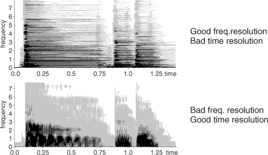
In this code we step through the input sound x, performing the FFT and the inverse-FFT on each frame. This operation involves selecting a number of samples from the sound signal and multiplying their value by a windowing function. The number of samples taken in every processing step is defined by the window size. It is a crucial parameter, especially if we take into account that the number of spectral samples that the DFT will yield at its output, corresponds to half the number of samples plus one of its input spread over half of the original sampling rate. We will not go into the details of the DFT mathematics that lead to this property, but it is very important to note that the longer the window, the more frequency resolution we will have. On the other hand, it is almost immediate to see the drawback of taking very long windows: the loss of temporal resolution. This phenomenon is known as the time vs. frequency resolution trade-off (see Figure 10.4). A more specific limitation of the window size has to do with choosing windows with odd sample lengths in order to guarantee even symmetry about the origin.
Figure 10.4 Time vs. frequency resolution trade-off.
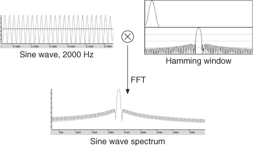
The type of window used also has a very strong effect on the qualities of the spectral representation we will obtain. At this point we should remember that a time-domain multiplication (as the one done between the signal and the windowing function), becomes a frequency-domain convolution between the Fourier transforms of each of the signals (see Figure 10.5). One may be tempted to forget about deciding on these matters and apply no window at all, just taking Msamples from the signal and feeding them to the chosen FFT algorithm. Even in that case, though, a rectangular window is being used, so the spectrum of the signal is being convolved with the transform of a rectangular pulse, a sinc-like function.
Figure 10.5 Effect of applying a window in the time domain.
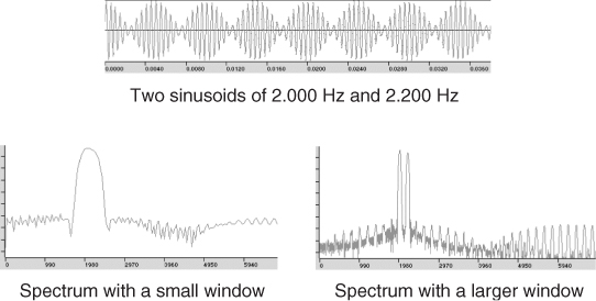
Two features of the transform of the window are especially relevant to whether a particular function is useful or not: the width of the main lobe, and the main to highest side lobe relation. The main lobe bandwidth is expressed in bins (spectral samples) and, in conjunction with the window size, defines the ability to distinguish two sinusoidal peaks (see Figure 10.6). The following formula expresses the relation that the window size, M, the main lobe bandwidth, Bs, and the sampling rate, fs, should meet in order to distinguish two sinusoids of frequencies fk and fk+1:
The amplitude relation between the main and the highest side lobe explains the amount of distortion a peak will receive from surrounding partials. It would be ideal to have a window with an extremely narrow main lobe and a very high main to secondary lobe relation. However, the inherent trade-off between these two parameters forces a compromise to be made.
Figure 10.6 Effect of the window size in distinguishing between two sinusoids.
Common windows that can be used in the analysis step are: rectangular, triangular, Kaiser-Bessel, Hamming, Hanning and Blackman-Harris. In the MATLAB code supplied, the user provides the analysis window, ![]() , to use as the input parameter.
, to use as the input parameter.
One may think that a possible way of overcoming the time/frequency trade-off is to add zeros at the extremes of the windowed signals to increase the frequency resolution, that is, to have the FFT size N larger than the window size M. This process is known as zero-padding and it represents an interpolation in the frequency domain. When we zero-pad a signal before the DFT process, we are not adding any information to its frequency representation, given that we are not adding any new signal samples. We will still not distinguish the sinusoids if Equation (10.6) is not satisfied, but we are indeed increasing the frequency resolution by adding intermediate interpolated bins. With zero-padding we are able to use sizes of windows that are not powers of two (requirement for using many FFT algorithm implementations) and we also obtain smoother spectra, which helps in the peak detection process, as later explained.
A final step before computing the FFT of the input signal is the circular shift already described in previous chapters. This data centering on the origin guarantees the preservation of zero-phase conditions in the analysis process.
Once the spectrum of a frame has been computed, the window must move to the next position in the input signal in order to take the next set of samples. The distance between the centers of two consecutive windows is known as hop size, H. If the hop size is smaller than the window size, we will be including some overlap, that is, some samples will be used more than once in the analysis process. In general, the more overlap, the smoother the transitions of the spectrum will be across time, but that is a computationally expensive process. The window type and the hop must be chosen in such a way that the resulting envelope adds approximately to a constant, following the equation
10.7 
A measure of the deviation of Aw from a constant is the difference between the maximum and minimum values for the envelope as a percentage of the maximum value. This measure is referred to as the amplitude deviation of the overlap factor. Variables should be chosen so as to keep this factor around or below 1%
10.8 ![]()
After the analysis process we reverse every single step done until now, starting by computing the inverse FFT of every spectrum. If Aw is equal to a constant the output signal, ![]() , will be identical to the original signal, x(n). Otherwise an amplitude deviation is manifested in the output sound, creating an audible distortion if the modulation is big enough.
, will be identical to the original signal, x(n). Otherwise an amplitude deviation is manifested in the output sound, creating an audible distortion if the modulation is big enough.
A solution to the distortion created by the overlap-add process is to divide the output signal by the envelope Aw. If some window overlap exists, this operation surely removes any modulation coming from the window overlap process. However, this does not mean that we can apply any combination of parameters. Dividing by small numbers should be generally avoided, since noise coming from numerical errors can be greatly boosted and introduce undesired artifacts at synthesis. In addition, we have to be especially careful at beginning and end sections of the processed audio, since Aw will have values around zero. The following code implements a complete STFT analysis/synthesis system using this approach.
M-file 10.2 (stftenv.m)
function y = stftenv(x, w, N, H)
% Authors: J. Bonada, X. Serra, X. Amatriain, A. Loscos
% Analysis/synthesis of a sound using the short-time Fourier transform
% x: input sound, w: analysis window (odd size), N: FFT size, H: hop size
% y: output sound
M = length(w); % analysis window size
N2 = N/2+1; % size of positive spectrum
soundlength = length(x); % length of input sound array
hM = (M-1)/2; % half analysis window size
pin = 1+hM; % initialize sound pointer in middle of analysis window
pend = soundlength-hM; % last sample to start a frame
fftbuffer = zeros(N,1); % initialize buffer for FFT
yw = zeros(M,1); % initialize output sound frame
y = zeros(soundlength,1); % initialize output array
yenv = y; % initialize window overlap envelope
w = w/sum(w); % normalize analysis window
while pin<pend
%-----analysis-----%
xw = x(pin-hM:pin+hM).*w(1:M); % window the input sound
fftbuffer(:) = 0; % reset buffer
fftbuffer(1:(M+1)/2) = xw((M+1)/2:M); % zero-phase window in fftbuffer
fftbuffer(N-(M-1)/2+1:N) = xw(1:(M-1)/2);
X = fft(fftbuffer); % compute FFT
mX = 20*log10(abs(X(1:N2))); % magnitude spectrum of positive frequencies
pX = unwrap(angle(X(1:N2))); % unwrapped phase spect. of positive freq.
%-----synthesis-----%
Y = zeros(N,1); % initialize spectrum
Y(1:N2) = 10.∧(mX/20).*exp(i.*pX); % generate positive freq.
Y(N2+1:N) = 10.∧(mX(N2-1:-1:2)/20).*exp(-i.*pX(N2-1:-1:2));
% generate neg.freq.
fftbuffer = real(ifft(Y)); % inverse FFT
yw(1:(M-1)/2) = fftbuffer(N-(M-1)/2+1:N); % undo zero-phase window
yw((M+1)/2:M) = fftbuffer(1:(M+1)/2);
y(pin-hM:pin+hM) = y(pin-hM:pin+hM) + yw(1:M); % output signal overlap-add
yenv(pin-hM:pin+hM) = yenv(pin-hM:pin+hM) + w; % window overlap-add
pin = pin+H; % advance sound pointer
end
yenvth = max(yenv)*0.1; % envelope threshold
yenv(find(yenv<yenvth)) = yenvth;
y = y./yenv;
The STFT process provides a suitable frequency-domain representation of the input signal. It is a far from trivial process and it is dependent on some low-level parameters closely related to the signal-processing domain. A little theoretical knowledge is required to understand the process, but we will also need practice to obtain the desired results for a given application.
10.3.2 Spectral Peaks
The sinusoidal model assumes that each spectrum of the STFT representation can be explained by the sum of a small number of sinusoids. Given enough frequency resolution, and thus, enough points in the spectrum, the spectrum of a sinusoid can be identified by its shape. Theoretically, a sinusoid that is stable both in amplitude and in frequency, a partial of the sound, has a well-defined frequency representation: the transform of the analysis window used to compute the Fourier transform. It should be possible to take advantage of this characteristic to distinguish partials from other frequency components. However, in practice this is rarely the case, since most natural sounds are not perfectly periodic and do not have nicely spaced and clearly defined peaks in the frequency domain. There are interactions between the different components, and the shapes of the spectral peaks cannot be detected without tolerating some mismatch. Only some instrumental sounds (e.g., the steady-state part of an oboe sound) are periodic enough and sufficiently free from prominent noise components that the frequency representation of a stable sinusoid can be recognized easily in a single spectrum (see Figure 10.7). A practical solution is to detect as many peaks as possible, with some small constraints, and delay the decision of what is a well-behaved partial to the next step in the analysis: the peak-continuation algorithm.
Figure 10.7 Peak detection: (a) peaks in magnitude spectrum; (b) peaks in the phase spectrum.
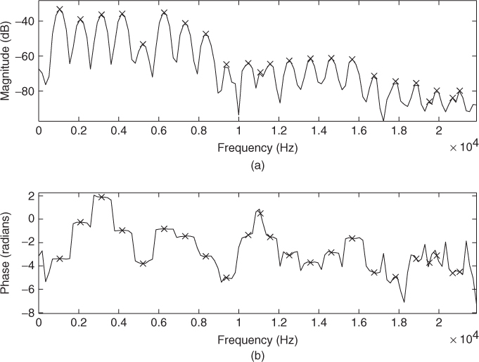
A peak is defined as a local maximum in the magnitude spectrum, and the only practical constraints to be made in the peak search are to have a local maximum over a certain frequency range and to have an amplitude greater than a given threshold.
Due to the sampled nature of the spectrum returned by the FFT, each peak is accurate only to within half a sample. A spectral sample represents a frequency interval of ![]() Hz, where fs is the sampling rate and N is the FFT size. Zero-padding in the time domain increases the number of spectral samples per Hz and thus increases the accuracy of the simple peak detection (see previous section). However, to obtain frequency accuracy on the level of 0.1% of the distance from the top of an ideal peak to its first zero crossing (in the case of a rectangular window), the zero-padding factor required is 1000.
Hz, where fs is the sampling rate and N is the FFT size. Zero-padding in the time domain increases the number of spectral samples per Hz and thus increases the accuracy of the simple peak detection (see previous section). However, to obtain frequency accuracy on the level of 0.1% of the distance from the top of an ideal peak to its first zero crossing (in the case of a rectangular window), the zero-padding factor required is 1000.
Here we include a modified version of the STFT code in which we only use the spectral peak values to perform the inverse-FFT.
M-file 10.3 (stpt.m)
function y = stpt(x, w, N, H, t)
% Authors: J. Bonada, X. Serra, X. Amatriain, A. Loscos
% Analysis/synthesis of a sound using the peaks
% of the short-time Fourier transform
% x: input sound, w: analysis window (odd size), N: FFT size, H: hop size,
% t: threshold in negative dB, y: output sound
M = length(w); % analysis window size
N2 = N/2+1; % size of positive spectrum
soundlength = length(x); % length of input sound aray
hM = (M-1)/2; % half analysis window size
pin = 1+hM; % initialize sound pointer at the middle of analysis window
pend = soundlength-hM; % last sample to start a frame
fftbuffer = zeros(N,1); % initialize buffer for FFT
yw = zeros(M,1); % initialize output sound frame
y = zeros(soundlength,1); % initialize output array
w = w/sum(w); % normalize analysis window
sw = hanning(M); % synthesis window
sw = sw./sum(sw);
while pin<pend
%-----analysis-----%
xw = x(pin-hM:pin+hM).*w(1:M); % window the input sound
fftbuffer(:) = 0; % reset buffer
fftbuffer(1:(M+1)/2) = xw((M+1)/2:M); % zero-phase fftbuffer
fftbuffer(N-(M-1)/2+1:N) = xw(1:(M-1)/2);
X = fft(fftbuffer); % compute the FFT
mX = 20*log10(abs(X(1:N2))); % magnitude spectrum of positive frequencies
pX = unwrap(angle(X(1:N2))); % unwrapped phase spectrum
ploc = 1 + find((mX(2:N2-1)>t) .* (mX(2:N2-1)>mX(3:N2)) ...
.* (mX(2:N2-1)>mX(1:N2-2))); % peaks
pmag = mX(ploc); % magnitude of peaks
pphase = pX(ploc); % phase of peaks
%-----synthesis-----%
Y = zeros(N,1); % initialize output spectrum
Y(ploc) = 10.∧(pmag/20).*exp(i.*pphase); % generate positive freq.
Y(N+2-ploc) = 10.∧(pmag/20).*exp(-i.*pphase); % generate negative freq.
fftbuffer = real(ifft(Y)); % real part of the inverse FFT
yw((M+1)/2:M) = fftbuffer(1:(M+1)/2); % undo zero phase window
yw(1:(M-1)/2) = fftbuffer(N-(M-1)/2+1:N);
y(pin-hM:pin+hM) = y(pin-hM:pin+hM) + H*N*sw.*yw(1:M); % overlap-add
pin = pin+H; % advance sound pointer
end
This code is mostly the same as the one used for the STFT, with the addition of a peak-detection step based on a magnitude threshold, that is, we only detect peaks whose magnitude is greater than a magnitude threshold specified by the user. Then, in the synthesis stage, the spectrum used to compute the inverse-FFT has values only at the bins of the peaks, and the rest have zero magnitude. It can be shown that each of these isolated bins is precisely the transform of a stationary sinusoid (of the frequency corresponding to the bin) multiplied by a rectangular window. Therefore, we smooth the resulting signal frame with a synthesis window, ![]() , to have smoother overlap-add behavior. Nevertheless, this implementation of a sinusoidal model is very simple and thus it is not appropriate for most applications. The next implementation is much more useful.
, to have smoother overlap-add behavior. Nevertheless, this implementation of a sinusoidal model is very simple and thus it is not appropriate for most applications. The next implementation is much more useful.
10.3.3 Spectral Sinusoids
In order to improve the implementation of the sinusoidal model, we have to use more refined methods for estimating the sinusoidal parameters and we have to implement an accurate synthesis of time-varying sinusoids. The diagram of the complete system is shown in Figure 10.8.
Figure 10.8 Block diagram of an analysis/synthesis system based on the sinusoidal model.
An efficient spectral interpolation scheme to better measure peak frequencies and magnitudes is to zero-pad only enough so that quadratic (or other simple) spectral interpolation, by using samples immediately surrounding the maximum-magnitude sample, suffices to refine the estimate to 0.1% accuracy. This is illustrated in Figure 10.9, where magnitudes are expressed in dB.
Figure 10.9 Parabolic interpolation in the peak-detection process.
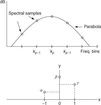
For a spectral peak located at bin kp, let us define ![]() ,
, ![]() and
and ![]() . The center of the parabola in bins is
. The center of the parabola in bins is ![]() , and the estimated amplitude
, and the estimated amplitude ![]() . Then the phase value of the peak is measured by reading the value of the unwrapped phase spectrum at the position resulting from the frequency of the peak. This is a good first approximation, but it is still not the ideal solution, since significant deviations in amplitude and phase can be found even in the case of simple linear frequency modulations.
. Then the phase value of the peak is measured by reading the value of the unwrapped phase spectrum at the position resulting from the frequency of the peak. This is a good first approximation, but it is still not the ideal solution, since significant deviations in amplitude and phase can be found even in the case of simple linear frequency modulations.
Here we include the code to perform the parabolic interpolation on the spectral peaks:
M-file 10.4 (peakinterp.m)
function [iploc, ipmag, ipphase] = peakinterp(mX, pX, ploc)
% Authors: J. Bonada, X. Serra, X. Amatriain, A. Loscos
% Parabolic interpolation of spectral peaks
% mX: magnitude spectrum, pX: phase spectrum, ploc: locations of peaks
% iploc, ipmag, ipphase: interpolated values
% note that ploc values are assumed to be between 2 and length(mX)-1
val = mX(ploc); % magnitude of peak bin
lval = mX(ploc-1); % magnitude of bin at left
rval= mX(ploc+1); % magnitude of bin at right
iploc = ploc + .5*(lval-rval)./(lval-2*val+rval); % center of parabola
ipmag = val-.25*(lval-rval).*(iploc-ploc); % magnitude of peaks
ipphase = interp1(1:length(pX),pX,iploc,'linear'), % phase of peaks
In order to decide whether a peak is a partial or not, it is sometimes useful to have a measure of how close its shape is to the ideal sinusoidal peak. With this idea in mind, different techniques have been used to improve the estimation of the spectral peak parameters [DH97]. More sophisticated methods make use of the spectral shape details and derive descriptors to distinguish between sinusoidal peaks, sidelobes and noise (e.g., [ZRR07]). Several other approaches target amplitude and frequency modulated sinusoids and are able to estimate their modulation parameters (e.g., [MB10]).
Peak Continuation
Once the spectral peaks of a frame have been detected, a peak-continuation algorithm can organize the peaks into frequency trajectories, where each trajectory models a time-varying sinusoid (see Figure 10.10).
Figure 10.10 Frequency trajectories resulting from the sinusoidal analysis of a vocal sound.
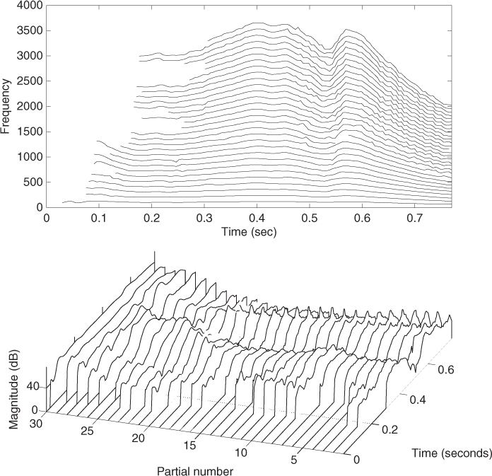
Several strategies have been explored during the last decades with the aim of connecting the sinusoidal components in the best possible way. McAulay and Quatieri proposed a simple sinusoidal continuation algorithm based on finding, for each spectral peak, the closest one in frequency in the next frame [MQ86]. Serra added to the continuation algorithm a set of frequency guides used to create sinusoidal trajectories [Ser89]. The frequency guide values were obtained from the peak values and their context, such as surrounding peaks and fundamental frequency. In the case of harmonic sounds, these guides were initialized according to the harmonic series of the estimated fundamental frequency. The trajectories were computed by assigning to each guide the closest peak in frequency.
There are peak-continuation methods based on hidden Markov models, which seem to be very valuable for tracking partials in polyphonic signals and complex inharmonic tones, for instance [DGR93]. Another interesting approach proposed by Peeters is to use a non-stationary sinusoid model, with linearly varying amplitude and frequency [Pee01]. Within that framework, the continuation algorithm focuses on the continuation of the value and first derivative for both amplitude and frequency polynomial parameters, combined with a measure of sinusoidality. Observation and transitions probabilities are defined, and a Viterbi algorithm is proposed for computing the sinusoidal trajectories.
Sinusoidal Synthesis
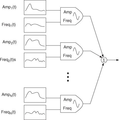
Once all spectral peaks are identified and ordered, we can start the synthesis part, thus generating the sinusoids that correspond to the connected peaks. The sinusoids can be generated in the time domain with additive synthesis, controlling the instantaneous frequency and amplitude of a bank of oscillators, as shown in Figure 10.11. For this case, we define synthesis frames ![]() as the segments determined by consecutive analysis times. For each synthesis frame, the instantaneous amplitude
as the segments determined by consecutive analysis times. For each synthesis frame, the instantaneous amplitude ![]() of an oscillator is obtained by linear interpolation of the surrounding amplitude estimations,
of an oscillator is obtained by linear interpolation of the surrounding amplitude estimations,
10.9 
where m = 0, 1, …, H − 1 is the time sample within the frame.
Figure 10.11 Additive synthesis block diagram.
The instantaneous phase is taken to be the integral of the instantaneous frequency, where the instantaneous radian frequency ![]() is obtained by linear interpolation,
is obtained by linear interpolation,
10.10 ![]()
and the instantaneous phase is
10.11 ![]()
Finally, the synthesis equation of a frame becomes
10.12 
where r is the oscillator index and Rl the number of sinusoids existing on the lth frame. The output sound ![]() is obtained by adding all frame segments together,
is obtained by adding all frame segments together,
10.13 
A much more efficient implementation of additive synthesis, where the instantaneous phase is not preserved, is based on the inverse-FFT [RD92]. While this approach loses some of the flexibility of the traditional oscillator-bank implementation, especially the instantaneous control of frequency and magnitude, the gain in speed is significant. This gain is based on the fact that a stationary sinusoid in the frequency domain is a sinc-type function, the transform of the window used, and on these functions not all the samples carry the same amplitude relevance. A sinusoid can be approximated in the spectral domain by computing the samples of the main lobe of the window transform, with the appropriate magnitude, frequency and phase values. We can then synthesize as many sinusoids as we want by adding these main lobes into the FFT buffer and performing an IFFT to obtain the resulting time-domain signal. By an overlap-add process we then get the time-varying characteristics of the sound.
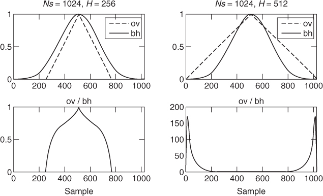
The synthesis frame rate is completely independent of the analysis one. In the implementation using the IFFT we want to have a frame rate high enough so as to preserve the temporal characteristics of the sound. As in all short-time-based processes we have the problem of having to make a compromise between time and frequency resolution. The window transform should have the fewest possible significant bins since this will be the number of points used to generate per sinusoid. A good window choice is the Blackman-Harris 92 dB (BH92) because its main lobe includes most of the energy. However, the problem is that such a window does not overlap perfectly to a constant in the time domain without having to use very high overlap factors, and thus very high frame rates. A solution to this problem is to undo the effect of the window by dividing the result of the IFFT by it (in the time domain) and applying an appropriate overlapping window (e.g., triangular) before performing the overlap-add process. This gives a good time-frequency compromise. However, it is desirable to use a hop-size significantly smaller than half the synthesis window length, so an overlap greater than 50%. Otherwise, large gains are applied at the window edges, which might introduce undesired artifacts at synthesis. This is illustrated in Figure 10.12, where a triangular window is used. Note that for a 50% overlap (Ns = 1024, H = 512) the gain at the window edges reaches values greater than 150.
Figure 10.12 Overlapping strategy based on dividing by the synthesis window and multiplying by an overlapping window. Undesired artifacts can be introduced at synthesis if the overlap is not significantly greater than 50%.
The zero-centered BH92 window is defined as
10.14 
where N is the window length. Since each cosine function is the sum of two complex exponentials, then its transform can be expressed by a sum of rectangular window transforms (or Dirichlet kernels) shifted to the cosine (positive and negative) frequencies. The following MATLAB code implements the computation of the Blackman-Harris 92 dB transform, which will be used to generate sinusoids in the spectral domain:
M-file 10.5 (genbh92lobe.m)
function y = genbh92lobe(x)
% Authors: J. Bonada, X. Serra, X. Amatriain, A. Loscos
% Calculate transform of the Blackman-Harris 92dB window
% x: bin positions to compute (real values)
% y: transform values
N = 512;
f = x*pi*2/N; % frequency sampling
df = 2*pi/N;
y = zeros(size(x)); % initialize window
consts = [.35875, .48829, .14128, .01168]; % window constants
for m=0:3
y = y + consts(m+1)/2*(D(f-df*m,N)+D(f+df*m,N)); % sum Dirichlet kernels
end
y = y/N/consts(1); % normalize
end
function y = D(x,N)
% Calculate rectangular window transform (Dirichlet kernel)
y = sin(N*x/2)./sin(x/2);
y(find(y∼=y))=N; % avoid NaN if x==0
end
Once we can generate a single sinusoid in the frequency domain, we can also generate a complete complex spectrum of a series of sinusoids from their frequency, magnitude and phase values.
M-file 10.6 (genspecsines.m)
function Y = genspecsines(ploc, pmag, pphase, N)
% Authors: J. Bonada, X. Serra, X. Amatriain, A. Loscos
% Compute a spectrum from a series of sine values
% iploc, ipmag, ipphase: sine locations, magnitudes and phases
% N: size of complex spectrum
% Y: generated complex spectrum of sines
Y =zeros(N,1); % initialize output spectrum
hN = N/2+1; % size of positive freq. spectrum
for i=1:length(ploc); % generate all sine spectral lobes
loc = ploc(i); % location of peak (zero-based indexing)
% it should be in range ]0,hN-1[
if (loc<=1||loc>=hN-1) continue; end; % avoid frequencies out of range
binremainder = round(loc)-loc;
lb = [binremainder-4:binremainder+4]'; % main lobe (real value) bins to read
lmag = genbh92lobe(lb)*10.∧(pmag(i)/20); % lobe magnitudes of the
% complex exponential
b = 1+[round(loc)-4:round(loc)+4]'; % spectrum bins to fill
% (1-based indexing)
for m=1:9
if (b(m)<1) % peak lobe croses DC bin
Y(2-b(m)) = Y(2-b(m)) + lmag(m)*exp(-1i*pphase(i));
elseif (b(m)>hN) % peak lobe croses Nyquist bin
Y(2*hN-b(m)) = Y(2*hN-b(m)) + lmag(m)*exp(-1i*pphase(i));
else % peak lobe in positive freq. range
Y(b(m)) = Y(b(m)) + lmag(m)*exp(1i*pphase(i)) ...
+ lmag(m)*exp(-1i*pphase(i))*(b(m)==1||b(m)==hN);
end
end
Y(hN+1:end) = conj(Y(hN-1:-1:2)); % fill the rest of the spectrum
end
In this code we place each sinusoid in its spectral location with the right amplitude and phase. What complicates the code a bit is the inclusion of special conditions when spectral lobe values cross the DC or the Nyquist bin locations.
Now that we have an improved implementation for detecting and synthesizing sinusoids we can implement a complete analysis/synthesis system based on this sinusoidal model.
M-file 10.7 (sinemodel.m)
function y = sinemodel(x, w, N, t)
% Authors: J. Bonada, X. Serra, X. Amatriain, A. Loscos
% Analysis/synthesis of a sound using the sinusoidal model
% x: input sound, w: analysis window (odd size), N: FFT size,
% t: threshold in negative dB, y: output sound
M = length(w); % analysis window size
Ns= 1024; % FFT size for synthesis (even)
H = 256; % analysis/synthesishop size
N2= N/2+1; % size of positive spectrum
soundlength = length(x); % length of input sound array
hNs = Ns/2; % half synthesis window size
hM = (M-1)/2; % half analysis window size
pin = max(hNs+1,1+hM); % initialize sound pointer to middle of analysis window
pend = soundlength-max(hNs,hM); % last sample to start a frame
fftbuffer = zeros(N,1); % initialize buffer for FFT
y = zeros(soundlength,1); % initialize output array
w = w/sum(w); % normalize analysis window
sw = zeros(Ns,1);
ow = triang(2*H-1); % overlapping window
ovidx = Ns/2+1-H+1:Ns/2+H; % overlap indexes
sw(ovidx) = ow(1:2*H-1);
bh = blackmanharris(Ns); % synthesis window
bh = bh ./ sum(bh); % normalize synthesis window
sw(ovidx) = sw(ovidx) ./ bh(ovidx);
while pin<pend
%-----analysis-----%
xw = x(pin-hM:pin+hM).*w(1:M); % window the input sound
fftbuffer(:) = 0; % reset buffer
fftbuffer(1:(M+1)/2) = xw((M+1)/2:M); % zero-phase window in fftbuffer
fftbuffer(N-(M-1)/2+1:N) = xw(1:(M-1)/2);
X = fft(fftbuffer); % compute the FFT
mX = 20*log10(abs(X(1:N2))); % magnitude spectrum of positive frequencies
pX = unwrap(angle(X(1:N/2+1))); % unwrapped phase spectrum
ploc = 1 + find((mX(2:N2-1)>t) .* (mX(2:N2-1)>mX(3:N2)) ...
.* (mX(2:N2-1)>mX(1:N2-2))); % find peaks
[ploc,pmag,pphase] = peakinterp(mX,pX,ploc); % refine peak values
%-----synthesis-----%
plocs = (ploc-1)*Ns/N; % adapt peak locations to synthesis FFT
Y = genspecsines(plocs,pmag,pphase,Ns); % generate spec sines
yw = fftshift(real(ifft(Y))); % time domain of sinusoids
y(pin-hNs:pin+hNs-1) = y(pin-hNs:pin+hNs-1) + sw.*yw(1:Ns); % overlap-add
pin = pin+H; % advance the sound pointer
end
The basic difference from the analysis/synthesis implementation based on spectral peaks is in the improvement of the peak detection using a parabolic interpolation, peakinterp, and on the implementation of the synthesis part. We now have a real additive synthesis section, which is completely independent of the analysis part. Thus it is no longer an FFT transform followed by its inverse-FFT transform. We could have implemented an additive synthesis in the time domain, but instead we have implemented an additive synthesis in the frequency domain, using the IFFT. We have fixed the synthesis FFT-size, 1204, and hop-size, 256, and they are independent of the analysis window type, window size and FFT size, which are defined by the user as input parameters of the function and are set depending on the sound to be processed. Since this method generates stationary sinusoids, there is no need to estimate the instantaneous phase or to interpolate the sinusoidal parameters, and therefore we can omit the peak-continuation algorithm. This would not be the case if we wanted to apply transformations.
10.3.4 Spectral Harmonics
A very useful constraint to be included in the sinusoidal model is to restrict the sinusoids to being harmonic partials, thus to assume that the input sound is monophonic and harmonic. With this constraint it should be possible to identify the fundamental frequency, F0, at each frame, and to have a much more compact and flexible spectral representation.
Given this restriction and the set of spectral peaks of a frame, with magnitude and frequency values for each one, there are many possible F0 estimation strategies, none of them perfect, e.g., [Hes83, MB94, Can98]. An obvious approach is to define F0 as the common divisor of the harmonic series that best explains the spectral peaks found in a given frame. For example, in the two-way mismatch procedure proposed by Maher and Beauchamp the estimated F0 is chosen as to minimize discrepancies between measured peak frequencies and the harmonic frequencies generated by trial values of F0. For each trial F0, mismatches between the harmonics generated and the measured peak frequencies are averaged over a fixed subset of the available peaks. This is a basic idea on top of which we can add features and tune all the parameters for a given family of sounds.
Many trade-offs are involved in the implementation of a F0 detection system and every application will require a clear design strategy. For example, the issue of real-time performance is a requirement with strong design implications. We can add context-specific optimizations when knowledge of the signal is available. Knowing, for instance, the frequency range of the F0 of a particular sound helps both the accuracy and the computational cost. Then, there are sounds with specific characteristics, like in a clarinet, where the even partials are softer than the odd ones. From this information, we can define a set of rules that will improve the performance of the estimator used.
In the framework of many spectral models there are strong dependencies between the fundamental-frequency detection step and many other analysis steps. For example, choosing an appropriate window for the Fourier analysis will facilitate detecting the fundamental frequency and, at the same time, getting a good fundamental frequency will assist other analysis steps, including the selection of an appropriate window. Thus, it could be designed as a recursive process.
The following MATLAB code implements the two-way mismatch algorithm for fundamental frequency detection:
M-file 10.8 (f0detectiontwm.m)
function f0 = f0detectiontwm(mX, fs, ploc, pmag, ef0max, minf0, maxf0)
% Authors: J. Bonada, X. Serra, X. Amatriain, A. Loscos
% Fundamental frequency detection function
% mX: magnitude spectrum, fs: sampling rate, ploc, pmag: peak loc and mag,
% ef0max: maximim error allowed, minf0: minimum f0, maxf0: maximum f0
% f0: fundamental frequency detected in Hz
N = length(mX)*2; % size of complex spectrum
nPeaks = length(ploc); % number of peaks
f0 = 0; % initialize output
if(nPeaks>3) % at least 3 peaks in spectrum for trying to find f0
nf0peaks = min(50,nPeaks); % use a maximum of 50 peaks
[f0,f0error] = TWM(ploc(1:nf0peaks),pmag(1:nf0peaks),N,fs,minf0,maxf0);
if (f0>0 && f0error>ef0max) % limit the possible error by ethreshold
f0 = 0;
end
end;
function [f0, f0error] = TWM (ploc, pmag, N, fs, minf0, maxf0)
% Two-way mismatch algorithm (by Beauchamp&Maher)
% ploc, pmag: peak locations and magnitudes, N: size of complex spectrum
% fs: sampling rate of sound, minf0: minimum f0, maxf0: maximum f0
% f0: fundamental frequency detected, f0error: error measure
pfreq = (ploc-1)/N*fs; % frequency in Hertz of peaks
[zvalue,zindex] = min(pfreq);
if (zvalue==0) % avoid zero frequency peak
pfreq(zindex) = 1;
pmag(zindex) = -100;
end
ival2 = pmag;
[Mmag1,Mloc1] = max(ival2); % find peak with maximum magnitude
ival2(Mloc1) = -100; % clear max peak
[Mmag2,Mloc2]= max(ival2); % find second maximum magnitude peak
ival2(Mloc2) = -100; % clear second max peak
[Mmag3,Mloc3]= max(ival2); % find third maximum magnitude peak
nCand = 3; % number of possible f0 candidates for each max peak
f0c = zeros(1,3*nCand); % initialize array of candidates
f0c(1:nCand)=(pfreq(Mloc1)*ones(1,nCand))./((nCand+1-(1:nCand))); % candidates
f0c(nCand+1:nCand*2)=(pfreq(Mloc2)*ones(1,nCand))./((nCand+1-(1:nCand)));
f0c(nCand*2+1:nCand*3)=(pfreq(Mloc3)*ones(1,nCand))./((nCand+1-(1:nCand)));
f0c = f0c((f0c<maxf0)&(f0c>minf0)); % candidates within boundaries
if (isempty(f0c)) % if no candidates exit
f0 = 0; f0error=100;
return
end
harmonic = f0c;
ErrorPM = zeros(fliplr(size(harmonic))); % initialize PM errors
MaxNPM = min(10,length(ploc));
for i=1:MaxNPM % predicted to measured mismatch error
difmatrixPM = harmonic' * ones(size(pfreq))';
difmatrixPM = abs(difmatrixPM-ones(fliplr(size(harmonic)))*pfreq'),
[FreqDistance,peakloc] = min(difmatrixPM,[],2);
Ponddif = FreqDistance .* (harmonic'.∧(-0.5));
PeakMag = pmag(peakloc);
MagFactor = 10.∧((PeakMag-Mmag1)./20);
ErrorPM = ErrorPM+(Ponddif+MagFactor.*(1.4*Ponddif-0.5));
harmonic = harmonic+f0c;
end
ErrorMP = zeros(fliplr(size(harmonic))); % initialize MP errors
MaxNMP = min(10,length(pfreq));
for i=1:length(f0c) % measured to predicted mismatch error
nharm = round(pfreq(1:MaxNMP)/f0c(i));
nharm = (nharm>=1).*nharm + (nharm<1);
FreqDistance = abs(pfreq(1:MaxNMP) - nharm*f0c(i));
Ponddif = FreqDistance.* (pfreq(1:MaxNMP).∧(-0.5));
PeakMag = pmag(1:MaxNMP);
MagFactor = 10.∧((PeakMag-Mmag1)./20);
ErrorMP(i) = sum(MagFactor.*(Ponddif+MagFactor.*(1.4*Ponddif-0.5)));
end
Error = (ErrorPM/MaxNPM) + (0.3*ErrorMP/MaxNMP); % total errors
[f0error, f0index] = min(Error); % get the smallest error
f0 = f0c(f0index); % f0 with the smallest error
There also exist many time-domain methods for estimating the fundamental frequency. It is worth mentioning the Yin algorithm, which offers excellent performance in many situations [CK02]. It is based on finding minima in the cumulative mean normalized difference function ![]() , defined as
, defined as
10.15 
10.16 
where x is the input signal, τ is the lag time, and W is the window size. Ideally, this function exhibits local minima at lag times corresponding to the fundamental period and its multiples. More refinements are described in the referenced article, although here we will only implement the basic procedure.
The following MATLAB code implements a simplified version of the Yin algorithm for fundamental frequency detection. We have included some optimizations in the calculations, such as performing sequential cumulative sums by adding and subtracting, respectively, the new and initial samples, or using the xcorr MATLAB function.
M-file 10.9 (f0detectionyin.m)
function f0 = f0detectionyin(x,fs,ws,minf0,maxf0)
% Authors: J. Bonada, X. Serra, X. Amatriain, A. Loscos
% Fundamental frequency detection function
% x: input signal, fs: sampling rate, ws: integration window length
% minf0: minimum f0, maxf0: maximum f0
% f0: fundamental frequency detected in Hz
maxlag = ws-2; % maximum lag
th = 0.1; % set threshold
d = zeros(maxlag,1); % init variable
d2 = zeros(maxlag,1); % init variable
% compute d(tau)
x1 = x(1:ws);
cumsumx = sum(x1.∧2);
cumsumxl = cumsumx;
xy = xcorr(x(1:ws*2),x1);
xy = xy(ws*2+1:ws*3-2);
for lag=0:maxlag-1
d(1+lag) = cumsumx + cumsumxl - 2*xy(1+lag);
cumsumxl = cumsumxl - x(1+lag).∧2 + x(1+lag+ws+1)∧2;
end
cumsum = 0;
% compute d'(tau)
d2(1) = 1;
for lag=1:maxlag-1
cumsum = cumsum + d(1+lag);
d2(1+lag) = d(1+lag)*lag./cumsum;
end
% limit the search to the target range
minf0lag = 1+round(fs./minf0); % compute lag corresponding to minf0
maxf0lag = 1+round(fs./maxf0); % compute lag corresponding to maxf0
if (maxf0lag>1 && maxf0lag<maxlag)
d2(1:maxf0lag) = 100; % avoid lags shorter than maxf0lag
end
if (minf0lag>1 && minf0lag<maxlag)
d2(minf0lag:end) = 100; % avoid lags larger than minf0lag
end
% find the best candidate
mloc = 1 + find((d2(2:end-1)<d2(3:end)).*(d2(2:end-1)<d2(1:end-2))); % minima
candf0lag = 0;
if (length(mloc)>0)
I = find(d2(mloc)<th);
if (length(I)>0)
candf0lag = mloc(I(1));
else
[Y,I2] = min(d2(mloc));
candf0lag = mloc(I2);
end
candf0lag = candf0lag; % this is zero-based indexing
if (candf0lag>1 & candf0lag<maxlag)
% parabolic interpolation
lval = d2(candf0lag-1);
val = d2(candf0lag);
rval= d2(candf0lag+1);
candf0lag = candf0lag + .5*(lval-rval)./(lval-2*val+rval);
end
end
ac = min(d2);
f0lag = candf0lag-1; % convert to zero-based indexing
f0 = fs./f0lag; % compute candidate frequency in Hz
if (ac > 0.2) % voiced/unvoiced threshold
f0 = 0; % set to unvoiced
end
When a relevant fundamental frequency is identified, we can decide to what harmonic number each of the peaks belongs and thus restrict the sinusoidal components to be only the harmonic ones. The diagram of the complete system is shown in Figure 10.13.
Figure 10.13 Block diagram of an analysis/synthesis system based on the harmonic sinusoidal model.
We can now add these steps into the implementation of the sinusoidal model represented in the previous section to implement a system that works just for harmonic sounds. Next is the complete MATLAB code for it.
M-file 10.10 (harmonicmodel.m)
function y = harmonicmodel(x, fs, w, N, t, nH, minf0, maxf0, f0et, maxhd)
% Authors: J. Bonada, X. Serra, X. Amatriain, A. Loscos
% Analysis/synthesis of a sound using the sinusoidal harmonic model
% x: input sound, fs: sampling rate, w: analysis window (odd size),
% N: FFT size (minimum 512), t: threshold in negative dB,
% nH: maximum number of harmonics, minf0: minimum f0 frequency in Hz,
% maxf0: maximim f0 frequency in Hz,
% f0et: error threshold in the f0 detection (ex: 5),
% maxhd: max. relative deviation in harmonic detection (ex: .2)
% y: output sound
M = length(w); % analysis window size
Ns= 1024; % FFT size for synthesis
H = 256; % hop size for analysis and synthesis
N2 = N/2+1; % size postive spectrum
soundlength = length(x); % length of input sound array
hNs = Ns/2; % half synthesis window size
hM = (M-1)/2; % half analysis window size
pin = max(hNS+1,1+hM); % initialize sound pointer to middle of analysis window
pend = soundlength-max(hNs,hM); % last sample to start a frame
fftbuffer = zeros(N,1); % initialize buffer for FFT
y = zeros(soundlength+Ns/2,1); % output sound
w = w/sum(w); % normalize analysis window
sw = zeros(Ns,1);
ow = triang(2*H-1); % overlapping window
ovidx = Ns/2+1-H+1:Ns/2+H; % overlap indexes
sw(ovidx) = ow(1:2*H-1);
bh = blackmanharris(Ns); % synthesis window
bh = bh ./ sum(bh); % normalize synthesis window
sw(ovidx) = sw(ovidx) ./ bh(ovidx);
while pin<pend
%-----analysis-----%
xw = x(pin-hM:pin+hM).*w(1:M); % window the input sound
fftbuffer(:) = 0; % reset buffer
fftbuffer(1:(M+1)/2) = xw((M+1)/2:M); % zero-phase window in fftbuffer
fftbuffer(N-(M-1)/2+1:N) = xw(1:(M-1)/2);
X = fft(fftbuffer); % compute the FFT
mX = 20*log10(abs(X(1:N2))); % magnitude spectrum
pX = unwrap(angle(X(1:N/2+1))); % unwrapped phase spectrum
ploc = 1 + find((mX(2:N2-1)>t) .* (mX(2:N2-1)>mX(3:N2)) ...
.* (mX(2:N2-1)>mX(1:N2-2))); % find peaks
[ploc,pmag,pphase] = peakinterp(mX,pX,ploc); % refine peak values
f0 = f0detectiontwm(mX,fs,ploc,pmag,f0et,minf0,maxf0); % find f0
hloc = zeros(nH,1); % initialize harmonic locations
hmag = zeros(nH,1)-100; % initialize harmonic magnitudes
hphase = zeros(nH,1); % initialize harmonic phases
hf = (f0>0).*(f0.*(1:nH)); % initialize harmonic frequencies
hi = 1; % initialize harmonic index
npeaks = length(ploc); % number of peaks found
while (f0>0 && hi<=nH && hf(hi)<fs/2) % find harmonic peaks
[dev,pei] = min(abs((ploc(1:npeaks)-1)/N*fs-hf(hi))); % closest peak
if ((hi==1 || ∼any(hloc(1:hi-1)==ploc(pei))) && dev<maxhd*hf(hi))
hloc(hi) = ploc(pei); % harmonic locations
hmag(hi) = pmag(pei); % harmonic magnitudes
hphase(hi) = pphase(pei); % harmonic phases
end
hi = hi+1; %increase harmonic index
end
hloc(1:hi-1) = (hloc(1:hi-1)∼=0).*((hloc(1:hi-1)-1)*Ns/N); % synth. locs
%-----synthesis-----%
Yh = genspecsines(hloc(1:hi-1),hmag,hphase,Ns); % generate sines
yh = fftshift(real(ifft(Yh))); % sines in time domain
y(pin-hNs:pin+hNs-1) = y(pin-hNs:pin+hNs-1) + sw.*yh(1:Ns); % overlap-add
pin = pin+H; % advance the input sound pointer
end
The basic differences from the previous implementation of the sinusoidal model are the detection of the F0 using the function f0detectiontwm, and the detection of the harmonic peaks by first generating a perfect harmonic series from the identified F0 and then searching the closest peaks for each harmonic value. This is a very simple implementation of a peak-continuation algorithm, but generally works for clean recordings of harmonic sounds. The major possible problem in using this implementation is in failing to detect the correct F0 for a given sound, causing the complete system to fail.
In the previous analysis/synthesis code we used the two-way mismatch algorithm, but we could perfectly use the Yin algorithm instead. A substantial difference between both is that whereas the first one operates on the spectra information, Yin receives a time-domain segment as input. If we prefer to use Yin, we can replace the line where f0detectiontwm was called in the previous code for the following ones. Note that the window length, yinws, has to be larger than the period corresponding to the minimum fundamental frequency to estimate.
M-file 10.11 (callyin.m)
% Authors: J. Bonada, X. Serra, X. Amatriain, A. Loscos
yinws = round(fs*0.015); % using approx. a 15 ms window for yin
yinws = yinws+mod(yinws,2); % make it even
yb = pin-yinws/2;
ye = pin+yinws/2+yinws;
if (yb<1 || ye>length(x)) % out of boundaries
f0 = 0;
else
f0 = f0detectionyin(x(yb:ye),fs,yinws,minf0,maxf0);
end
10.3.5 Spectral Harmonics Plus Residual
Once we have identified the harmonic partials of a sound, we can subtract them from the original signal and obtain a residual component. This subtraction can be done either in the time domain or in the frequency domain. A time-domain approach requires first to synthesize a time signal from the sinusoidal trajectories, while if we stay in the frequency domain, we can perform the subtraction directly in the already computed magnitude spectrum. For the time-domain subtraction, the phases of the original sound have to be preserved in the synthesized signal, thus we have to use a type of additive synthesis with which we can control the instantaneous phase. This is a type of synthesis that is computationally quite expensive. On the other hand, the sinusoidal subtraction in the spectral domain is in many cases computationally simpler, and can give similar results, in terms of accuracy, as the time-domain implementation. We have to understand that the sinusoidal information obtained from the analysis is very much under-sampled, since for every sinusoid we only have the value at the tip of the peaks, and thus we have to re-generate all the spectral samples that belong to the sinusoidal peak to be subtracted.
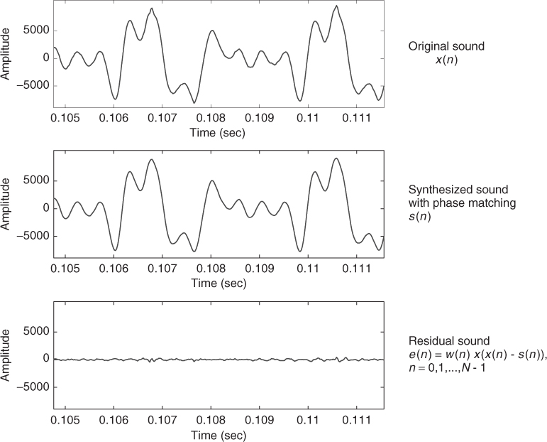
Once we have, either the residual spectrum or the residual time signal, it is useful to study it in order to check how well the partials of the sound were subtracted and therefore analyzed. If partials remain in the residual, the possibilities for transformations will be reduced, since these are not adequate for typical residual models. In this case, we should re-analyze the sound until we get a good residual, free of harmonic partials. Ideally, for monophonic signals, the resulting residual should be as close as possible to a stochastic signal.
The first step in obtaining the residual is to synthesize the sinusoids obtained as the output of the harmonic analysis. For a time-domain subtraction (see Figure 10.14) the synthesized signal will reproduce the instantaneous phase and amplitude of the partials of the original sound with a bank of oscillators. Different approaches are possible for computing the instantaneous phase, for instance [MQ86], thus being able to synthesize one frame which goes smoothly from the previous to the current frame with each sinusoid accounting for both the rapid phase changes (frequency) and the slowly varying phase changes. However, an efficient implementation can also be obtained by frequency-domain subtraction, where a spectral representation of stationary sinusoids is generated [RD92].
Figure 10.14 Time-domain subtraction.
Next is an implementation of a complete system using a harmonic plus residual model and based on subtracting the harmonic component in the frequency domain (see the diagram in Figure 10.15).
M-file 10.12 (hprmodel.m)
function [y,yh,yr] = hprmodel(x,fs,w,N,t,nH,minf0,maxf0,f0et,maxhd)
% Authors: J. Bonada, X. Serra, X. Amatriain, A. Loscos
% Analysis/synthesis of a sound using the sinusoidal harmonic model
% x: input sound, fs: sampling rate, w: analysis window (odd size),
% N: FFT size (minimum 512), t: threshold in negative dB,
% nH: maximum number of harmonics, minf0: minimum f0 frequency in Hz,
% maxf0: maximim f0 frequency in Hz,
% f0et: error threshold in the f0 detection (ex: 5),
% maxhd: max. relative deviation in harmonic detection (ex: .2)
% y: output sound, yh: harmonic component, yr: residual component
M = length(w); % analysis window size
Ns = 1024; % FFT size for synthesis
H = 256; % hop size for analysis and synthesis
N2 = N/2+1; % half-size of spectrum
soundlength = length(x); % length of input sound array
hNs = Ns/2; % half synthesis window size
hM = (M-1)/2; % half analysis window size
pin = max(hNs+1,1+hM); % initialize sound pointer to middle of analysis window
pend = soundlength-max(hM,hNs); % last sample to start a frame
fftbuffer = zeros(N,1); % initialize buffer for FFT
yh = zeros(soundlength+Ns/2,1); % output sine component
yr = zeros(soundlength+Ns/2,1); % output residual component
w = w/sum(w); % normalize analysis window
sw = zeros(Ns,1);
ow = triang(2*H-1); % overlapping window
ovidx = Ns/2+1-H+1:Ns/2+H; % overlap indexes
sw(ovidx) = ow(1:2*H-1);
bh = blackmanharris(Ns); % synthesis window
bh = bh ./ sum(bh); % normalize synthesis window
wr = bh; % window for residual
sw(ovidx) = sw(ovidx) ./ bh(ovidx);
while pin<pend
%-----analysis-----%
xw = x(pin-hM:pin+hM).*w(1:M); % window the input sound
fftbuffer(:) = 0; % reset buffer
fftbuffer(1:(M+1)/2) = xw((M+1)/2:M); % zero-phase window in fftbuffer
fftbuffer(N-(M-1)/2+1:N) = xw(1:(M-1)/2);
X = fft(fftbuffer); % compute the FFT
mX = 20*log10(abs(X(1:N2))); % magnitude spectrum
pX = unwrap(angle(X(1:N/2+1))); % unwrapped phase spectrum
ploc = 1 + find((mX(2:N2-1)>t) .* (mX(2:N2-1)>mX(3:N2)) ...
.* (mX(2:N2-1)>mX(1:N2-2))); % find peaks
[ploc,pmag,pphase] = peakinterp(mX,pX,ploc); % refine peak values
f0 = f0detectiontwm(mX,fs,ploc,pmag,f0et,minf0,maxf0); % find f0
hloc = zeros(nH,1); % initialize harmonic locations
hmag = zeros(nH,1)-100; % initialize harmonic magnitudes
hphase = zeros(nH,1); % initialize harmonic phases
hf = (f0>0).*(f0.*(1:nH)); % initialize harmonic frequencies
hi = 1; % initialize harmonic index
npeaks = length(ploc); % number of peaks found
while (f0>0 && hi<=nH && hf(hi)<fs/2) % find harmonic peaks
[dev,pei] = min(abs((ploc(1:npeaks)-1)/N*fs-hf(hi))); % closest peak
if ((hi==1 || ∼any(hloc(1:hi-1)==ploc(pei))) && dev<maxhd*hf(hi))
hloc(hi) = ploc(pei); % harmonic locations
hmag(hi) = pmag(pei); % harmonic magnitudes
hphase(hi) = pphase(pei); % harmonic phases
end
hi = hi+1; % increase harmonic index
end
hloc(1:hi-1) = (hloc(1:hi-1)∼=0).*((hloc(1:hi-1)-1)*Ns/N); % synth. locs
ri= pin-hNs; % input sound pointer for residual analysis
xr = x(ri:ri+Ns-1).*wr(1:Ns); % window the input sound
Xr = fft(fftshift(xr)); % compute FFT for residual analysis
%-----synthesis-----%
Yh = genspecsines(hloc(1:hi-1),hmag,hphase,Ns); % generate sines
Yr = Xr-Yh; % get the residual complex spectrum
yhw = fftshift(real(ifft(Yh))); % sines in time domain using inverse FFT
yrw = fftshift(real(ifft(Yr))); % residual in time domain using inverse FFT
yh(ri:ri+Ns-1) = yh(ri:ri+Ns-1)+yhw(1:Ns).*sw; % overlap-add for sines
yr(ri:ri+Ns-1) = yr(ri:ri+Ns-1)+yrw(1:Ns).*sw; % overlap-add for residual
pin = pin+H; % advance the sound pointer
end
y= yh+yr; % sum sines and residual
Figure 10.15 Block diagram of the harmonic plus residual analysis/synthesis system.
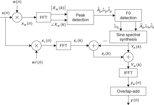
In order to subtract the harmonic component from the original sound in the frequency domain we have added a parallel FFT analysis of the input sound, with an analysis window which is the same than the one used in the synthesis step. Thus we can get a residual spectrum, Xres, and by simply computing its inverse FFT we obtain the time-domain residual. The synthesized signal, ![]() , is the sum of the harmonic and residual components. The function also returns the harmonic and residual components as separate signals.
, is the sum of the harmonic and residual components. The function also returns the harmonic and residual components as separate signals.
10.3.6 Spectral Harmonics Plus Stochastic Residual
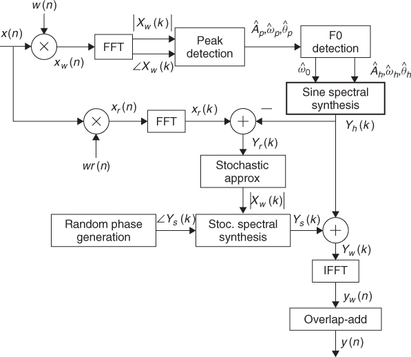
Once we have a decomposition of a sound into harmonic and residual components, from the residual signal we can continue our modeling strategy towards a more compact and flexible representation. When the harmonics have been well identified and subtracted the residual can be considered a stochastic signal ready to be parameterized. To model, or parameterize, the relevant parts of the residual component of a musical sound, such as the bow noise in stringed instruments or the breath noise in wind instruments, we need good time resolution and we can give up some of the frequency resolution required for modeling the harmonic component. Given the window requirements for the STFT analysis the harmonic component cannot maintain the sharpness of the attacks, because, even if a high frame rate is used we are forced to use a long enough window, and this size determines most of the time resolution. However, once the harmonic subtraction has been done, the temporal resolution to analyze the residual component can be improved by using a different analysis window (see Figure 10.16).
Figure 10.16 Block diagram of an analysis/synthesis system based on a harmonic plus stochastic model.
Since the harmonic analysis has been performed using long windows, the subtraction of the harmonic component generated from that analysis might result in smearing of the sharp discontinuities, like note attacks, which remain in the residual component. We can fix this smearing effect of the residual and try to preserve the sharpness of the attacks of the original sound. For example, the resulting time-domain residual can be compared with the original waveform and its amplitude re-scaled whenever the residual has a greater energy than the original waveform. Then the stochastic analysis is performed on this modified residual. We can also compare the synthesized harmonic signal with the original sound and whenever this signal has a greater energy than the original waveform it means that a smearing of the harmonic component has been produced. This can be fixed a bit by scaling the amplitudes of the harmonic analysis in the corresponding frame using the difference between the original sound and the harmonic signal.
Residual Analysis
One of the underlying assumptions of the sinusoidal plus residual model is that the residual is a stochastic signal. Such an assumption implies that the residual is fully described by its amplitude and its general frequency characteristics (see Figure 10.17). It is unnecessary to keep either the instantaneous phase or the exact spectral shape information. Based on this, a frame of the stochastic residual can be completely characterized by a filter, i.e., this filter encodes the amplitude and general frequency characteristics of the residual. The representation of the residual in the overall sound will be a sequence of these filters, i.e., a time-varying filter.
Figure 10.17 (a) Original spectrum. (b) Residual spectrum and approximation.
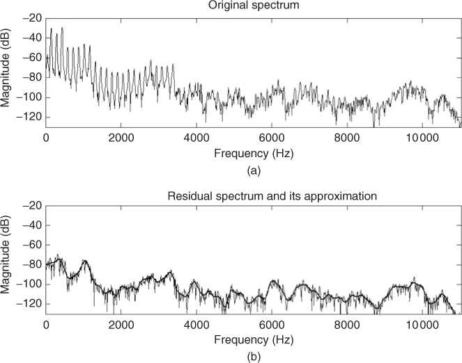
The filter design problem is generally solved by performing some sort of curve fitting in the magnitude spectrum of the current frame [Str80, Sed88]. Standard techniques are: spline interpolation [Cox71], the method of least squares [Sed88], or straight-line approximations.
One way to carry out the line-segment approximation is to step through the magnitude spectrum and find local maxima in each of several defined sections, thus giving equally spaced points in the spectrum that are connected by straight lines to create the spectral envelope. The number of points gives the accuracy of the fit, and that can be set depending on the sound complexity. Other options are to have unequally spaced points, for example, logarithmically spaced, or spaced according to other perceptual criteria.
Another practical alternative is to use a type of least squares approximation called linear predictive coding, LPC [Mak75, MG75]. LPC is a popular technique used in speech research for fitting an nth-order polynomial to a magnitude spectrum. For our purposes, the line-segment approach is more flexible than LPC, and although LPC results in less analysis points, the flexibility is considered more important. For a comprehensive collection of different approximation techniques of the residual component see [Goo97].
Residual Synthesis
From the stochastic model, parameterization of the residual component, we can synthesize a signal that should preserve the perceptually relevant characteristic of the residual signal. Like the sinusoidal synthesis, this synthesis can either be done in the time or in the frequency domains. Here we present a frequency-domain implementation. We generate a complete complex spectrum at each synthesis frame from the magnitude spectral envelope that approximated the residual.
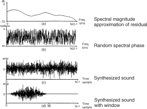
The synthesis of a stochastic signal from the residual approximation can be understood as the generation of noise that has the frequency and amplitude characteristics described by the spectral magnitude envelopes. The intuitive operation is to filter white noise with these frequency envelopes, that is, performing a time-varying filtering, which is generally implemented by the time-domain convolution of white noise with the impulse response corresponding to the spectral envelope of a frame. We can instead approximate it in the frequency domain (see Figure 10.18) by creating a magnitude spectrum from the estimated envelope, or its transformation, and generating a random phase spectrum with new values at each frame in order to avoid periodicity.
Figure 10.18 Stochastic synthesis.
Once the harmonic and stochastic spectral components have been generated, we can compute the IFFT of each one, and add the resulting time-domain signals. A more efficient alternative is to directly add the spectrum of the residual component to that of the sinusoids. However, in this case we need to worry about windows. In the process of generating the noise spectrum there has not been any window applied, since the data was added directly into the spectrum without any smoothing consideration, but in the sinusoidal synthesis we have used a Blackman-Harris 92 dB, which is undone in the time domain after the IFFT. Therefore we should apply the same window in the noise spectrum before adding it to the sinusoidal spectrum. Convolving the transform of the Blackman-Harris 92 dB by the noise spectrum accomplishes this, and there is only the need to use the main lobe of the window since that includes most of its energy. This is implemented quite efficiently because it only involves a few bins and the window is symmetric. Then we can use a single IFFT for the combined spectrum. Finally in the time domain we undo the effect of the Blackman-Harris 92 dB and impose the triangular window. By an overlap-add process we combine successive frames to get the time-varying characteristics of the sound. In the implementation shown later on this is not done in order to be able to output the two components separately and thus be able to hear the harmonic and the stochastic components of the sound.
Several other approaches have been used for synthesizing the output of a sinusoidal plus stochastic analysis. These techniques, though, include modifications to the model as a whole. For instance, [FHC00] proposes to link the stochastic components to each sinusoid by using stochastic modulation to spread spectral energy away from the sinusoid's center frequency. With this technique each partial has an extra parameter, the bandwidth coefficient, which sets the balance between noise and sinusoidal energy.
Below is the code of a complete system using a harmonic plus stochastic model:
M-file 10.13 (hpsmodel.m)
function [y,yh,ys] = hpsmodel(x,fs,w,N,t,nH,minf0,maxf0,f0et,maxhd,stocf)
% Authors: J. Bonada, X. Serra, X. Amatriain, A. Loscos
% Analysis/synthesis of a sound using the sinusoidal harmonic model
% x: input sound, fs: sampling rate, w: analysis window (odd size),
% N: FFT size (minimum 512), t: threshold in negative dB,
% nH: maximum number of harmonics, minf0: minimum f0 frequency in Hz,
% maxf0: maximim f0 frequency in Hz,
% f0et: error threshold in the f0 detection (ex: 5),
% maxhd: max. relative deviation in harmonic detection (ex: .2)
% stocf: decimation factor of mag spectrum for stochastic analysis
% y: output sound, yh: harmonic component, ys: stochastic component
M = length(w); % analysis window size
Ns = 1024; % FFT size for synthesis
H = 256; % hop size for analysis and synthesis
N2 = N/2+1; % half-size of spectrum
soundlength = length(x); % length of input sound array
hNs = Ns/2; % half synthesis window size
hM = (M-1)/2; % half analysis window size
pin = max(hNs+1,1+hM); % initialize sound pointer to middle of analysis window
pend = soundlength-max(hM,hNs); % last sample to start a frame
fftbuffer = zeros(N,1); % initialize buffer for FFT
yh = zeros(soundlength+Ns/2,1); % output sine component
ys = zeros(soundlength+Ns/2,1); % output residual component
w = w/sum(w); % normalize analysis window
sw = zeros(Ns,1);
ow = triang(2*H-1); % overlapping window
ovidx = Ns/2+1-H+1:Ns/2+H; % overlap indexes
sw(ovidx) = ow(1:2*H-1);
bh = blackmanharris(Ns); % synthesis window
bh = bh ./ sum(bh); % normalize synthesis window
wr = bh; % window for residual
sw(ovidx) = sw(ovidx) ./ bh(ovidx);
sws = H*hanning(Ns)/2; % synthesis window for stochastic
while pin<pend
%-----analysis-----%
xw = x(pin-hM:pin+hM).*w(1:M); % window the input sound
fftbuffer(:) = 0; % reset buffer
fftbuffer(1:(M+1)/2) = xw((M+1)/2:M); % zero-phase window in fftbuffer
fftbuffer(N-(M-1)/2+1:N) = xw(1:(M-1)/2);
X = fft(fftbuffer); % compute the FFT
mX = 20*log10(abs(X(1:N2))); % magnitude spectrum
pX = unwrap(angle(X(1:N/2+1))); % unwrapped phase spectrum
ploc = 1 + find((mX(2:N2-1)>t) .* (mX(2:N2-1)>mX(3:N2)) ...
.* (mX(2:N2-1)>mX(1:N2-2))); % find peaks
[ploc,pmag,pphase] = peakinterp(mX,pX,ploc); % refine peak values
f0 = f0detectiontwm(mX,fs,ploc,pmag,f0et,minf0,maxf0); % find f0
hloc = zeros(nH,1); % initialize harmonic locations
hmag = zeros(nH,1)-100; % initialize harmonic magnitudes
hphase = zeros(nH,1); % initialize harmonic phases
hf = (f0>0).*(f0.*(1:nH)); % initialize harmonic frequencies
hi = 1; % initialize harmonic index
npeaks = length(ploc); % number of peaks found
while (f0>0 && hi<=nH && hf(hi)<fs/2) % find harmonic peaks
[dev,pei] = min(abs((ploc(1:npeaks)-1)/N*fs-hf(hi))); % closest peak
if ((hi==1 || ∼any(hloc(1:hi-1)==ploc(pei))) && dev<maxhd*hf(hi))
hloc(hi) = ploc(pei); % harmonic locations
hmag(hi) = pmag(pei); % harmonic magnitudes
hphase(hi) = pphase(pei); % harmonic phases
end
hi = hi+1; % increase harmonic index
end
hloc(1:hi-1) = (hloc(1:hi-1)∼=0).*((hloc(1:hi-1)-1)*Ns/N); % synth. locs
ri= pin-hNs; % input sound pointer for residual analysis
xr = x(ri:ri+Ns-1).*wr(1:Ns); % window the input sound
Xr = fft(fftshift(xr)); % compute FFT for residual analysis
Yh = genspecsines(hloc(1:hi-1),hmag,hphase,Ns); % generate sines
Yr = Xr-Yh; % get the residual complex spectrum
mYr = abs(Yr(1:Ns/2+1)); % magnitude spectrum of residual
mYsenv = decimate(mYr,stocf); % decimate the magnitude spectrum
%-----synthesis-----%
mYs = interp(mYsenv,stocf); % interpolate to original size
roffset = ceil(stocf/2)-1; % interpolated array offset
mYs = [ mYs(1)*ones(roffset,1); mYs(1:Ns/2+1-roffset) ];
pYs = 2*pi*rand(Ns/2+1,1); % generate phase random values
mYs1 = [mYs(1:Ns/2+1); mYs(Ns/2:-1:2)]; % create magnitude spectrum
pYs1 = [pYs(1:Ns/2+1); -1*pYs(Ns/2:-1:2)]; % create phase spectrum
Ys = mYs1.*cos(pYs1)+1i*mYs1.*sin(pYs1); % compute complex spectrum
yhw = fftshift(real(ifft(Yh))); % sines in time domain using IFFT
ysw = fftshift(real(ifft(Ys))); % stoc. in time domain using IFFT
yh(ri:ri+Ns-1) = yh(ri:ri+Ns-1)+yhw(1:Ns).*sw; % overlap-add for sines
ys(ri:ri+Ns-1) = ys(ri:ri+Ns-1)+ysw(1:Ns).*sws; % overlap-add for stoch.
pin = pin+H; % advance the sound pointer
end
y= yh+ys; % sum sines and stochastic
This code extends the implementation of the harmonic plus residual with the approximation of the residual and the synthesis of a stochastic signal. It first approximates the residual magnitude spectrum using the function decimate from MATLAB. This function resamples a data array at a lower rate after lowpass filtering and using a decimation factor, stocf, given by the user. At synthesis a complete magnitude spectrum is generated by interpolating the approximated envelope using the function interp. This is a MATLAB function that re-samples data at a higher rate using lowpass interpolation. The corresponding phase spectrum is generated with a random number generator, the function rand. The output signal, y(n), is the sum of the harmonic and the stochastic components.