12.4 Electromechanical Effects

A rather special family of audio effects consists of those which employ mechanical elements in conjunction with analog electronics—though many classic effects rely on such components (such as, for example, the Leslie speaker, or tape delays), for some problems in the world of virtual analog, an involved treatment of the mechanical part of the effect is necessary, in order to be able to capture the perceptually salient quality of the effect. This is particularly the case for electromechanical artificial reverberation, which exhibits an extremely complex response. Two interesting cases, namely plate and spring reverberation, will be briefly described here.

The attribute of these devices which distinguishes them from other electromechanical effects is that the mechanical components cannot be modelled as “lumped” structurally, a spring or a plate occupies space, and its vibration pattern varies from one point to the next. It is precisely the distributed character of these components which gives these effects their complex sound—and which, at the same time, requires a somewhat different approach to emulation. One must now think of the behavior of the component in terms of various different modes of vibration, or in terms of waves which require finite propagation times, just like real acoustic spaces. Indeed, spring and plate reverbs were originally intended as convenient substitutes for real room reverbs—but developed a loyal audience of their own. Originally, such popularity was probably in spite of this distinction, but as such units have become scarce, convenient digital substitutes for these sometimes bulky and damage-prone units have become sought-after—and make for a fascinating application of virtual analog modeling!

Distributed modeling is seen only rarely in the world of digital audio effects, but plays, of course, a central role in sound synthesis based on physical models of musical instruments—a topic which is too broad to fit into this volume! In this short section, some of the basics of distributed modeling for electromechanical elements are covered, from a high-level perspective, focusing on the nature of the phenomena involved, and some simulation techniques (and in particular, finite difference schemes). It's probably worth mentioning that distributed modeling can be a lot more expensive, in terms of number-crunching, than other analog effect emulation—which is true of any digital reverberation algorithm. But, these days, standard computer hardware is becoming powerful enough to tackle these modeling problems in real-time, or something close to it.

12.4.1 Room Reverberation and the 3D Wave Equation

When looking at artificial reverberation techniques, it's useful to first take a look at the behaviour of real rooms—to understand the ways in which electromechanical effects attempt to emulate this real-world effect, and, more importantly, how they differ!

In air, to a very good approximation, waves travel at a constant speed, here referred to as c. c has a mild dependence on temperature, and is approximately 343 m/s at atmospheric pressure, and near room temperature [FR91]. From a given acoustic point source, waves travel uniformly in all directions (isotropically) at this speed, and there is a reduction in amplitude as the waves spread out. Formally, to a very good approximation, the time evolution of a pressure field in three dimensions may be described by the wave equation,

12.20

where here, p(x, y, z, t) is the pressure at spatial coordinates x, y and z, and at time t. ∇2 is the 3D Laplacian operator. For more on this equation, see [MI68].

A key concept in all distributed modeling for linear systems is a dispersion relation, relating angular frequency ω (in radians/sec) to a vector wavenumber β (measured in units of m−1) for a wave component of the solution. Such a component will be of the form

12.21

in 3D, and the dispersion relation for the wave equation above takes the following form,

12.22

It turns out to be convenient to use ω and β here, but one could equally well write this relationship in terms of frequency f = ω/2π and wavelength λ = 2π/|β|—the above dispersion relation then becomes the familiar expression c = λf. In the case of the wave equation, this expression is of a very simple form; for other systems it will not be, and often, even for a single system, there may be many such relations, which may not be expressible in simple closed form. The dispersion relation, in general, yields a huge amount of information about the behavior of a system which is very important acoustically. When a system's geometry is specified, one can say a great deal not only about acoustic attributes such as echo density and mode density, but also about how much computational power will be required to perform a digital emulation!

Expressions for wave speed as a function of frequency may be derived from a dispersion relation as

12.23

where vphase is the phase velocity, or propagation speed of a wave at wavenumber β, and vgroup is the group, or packet velocity. In the case of rooms, from the dispersion relation given above, these speeds are both c. Such wave propagation is often referred to as non dispersive; all disturbances propagate at the same speed, regardless of wavelength or frequency. In the present case of wave propagation in air, it also implies that waveforms which propagate from one point to another preserve shape, or remain coherent during propagation.

When a given delimited acoustic space is defined, the obvious acoustic effect is that of echoes. For a room with reflective walls, a typical response consists of series of distinct echoes (early reflections) which are perceptually distinct, and which serve as localization cues, followed by increasingly dense late reflections, and, finally when reflections become so dense so as to be not perceptually distinct, a reverberant tail. It is room geometry which gives acoustic responses their characteristic complexity—and this is definitely not the case for plate and spring reverberation, which emulate this response using relatively simple structures.

Digital emulation of 3D acoustic spaces through the direct solution of the wave equation is a daunting task, from the point of view of computational complexity (though it is an active research topic [Bot95, MKMS07], which will surely eventually bear fruit). In fact, by further examination of the dispersion relation one may arrive at bounds on computational cost: for any simulation of the 3D wave equation over a space of volume V, and which is intended to produce an approximation to the response over a band of frequencies from 0 Hz, to fs/2 Hz, for some frequency fs (i.e., an audio sample rate), the amount of memory required will be approximately

12.24

where the constant of proportionality depends on the particular method employed. For c = 340, and at at typical audio rate fs = 48 kHz, and for even a moderately sized room (V = 1000 m3), this can be very large indeed—here, for (say) a finite difference scheme N = 2.8 × 109! Because arithmetic operations will presumably be performed on all the data, locally, at the audio rate, the operation count will be on the order of N × fs flops, which is approaching the petaflop range. For more on the topic of computational complexity estimates in physical audio applications, see [Bil09].

Most reverberation techniques are thus based around perceptual simplifications, as described in detail in Chapter 5. In industrial acoustical applications, methods based on the image source method [AB79] are popular, and rely on simplified models of reflection from surfaces; in audio, feedback delay networks [Puc82, Roc97, JC91], which are very efficient, but not based on direct solution of the 3D wave equation, are commonly employed.

12.4.2 Plates and Plate Reverberation

Plate reverberation was originally intended as a convenient means of applying a reverberant effect to a recorded sound [Kuh58], long before the advent of digital reverberation. Such effects were extensively researched and eventually commericialized, with the EMT-140 the most successful resulting product. The basic operation of such a unit is relatively simple: a metal plate, normally rectangular, made of steel and supported by a frame is driven by an input signal through an actuator, and outputs are read at a pair of pickups. See Figure 12.15(a). Such a device is often complemented by adjustible absorbing plates which allow for some control over the decay time. The response of a plate is generally quite different from that of room acoustic reverberation—distinct relections are notably absent, and the response as a whole has a smooth noise-like character.

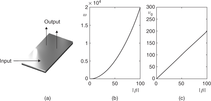
Figure 12.15 (a) A metal plate, driven by an input signal, and from which output(s) are read at distinct locations.(b) Dispersion relation, and (c) group velocity for a thin plate.

A given plate is characterized by its density ρ, in kg/m3, Young's modulus E, in kg/s2m, Poisson's ratio ν (dimensionless), and geometrical properties such as its thickness H in m, and its surface area A in m2, as well as the particular boundary conditions. A typical reverberation unit is constructed from steel, with a thickness of approximately 0.5 mm, and with a surface area of approximately 2 m2 (other materials and dimensions are also in use—the much smaller EMT 240 unit employs thin gold foil instead of steel). Usually the edges are very nearly free to vibrate, except for at the plate supports. For a sufficiently thin lossless plate, the equation of motion may be written succinctly as

12.25

where ∇2 is the 2D Laplacian operator defined, in Cartesian coordinates (x, y), as

12.26

For more on the physics of plates, see, e.g., [FR91, Gra75, MI68].

The dispersion relation for a plate is very different from that corresponding to wave propagation in air,

12.27

where . Now, the phase and group velocities are no longer constant,

12.28

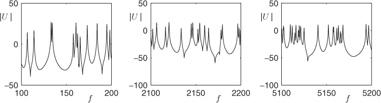
See Figure 12.15 (b) and (c). As a result, wave propagation is dispersive, and highly so. See Figure 12.16, showing the time evolution of plate displacement in response to a pulse. Notice in particular that the high-frequency components of the pulse travel more quickly than the low-frequency components—and thus the pulse rapidly loses coherence as it travels. Another related distinction between plate and room responses is the mode density, which is roughly constant in the case of the plate, but which increases as the square of frequency for a room. See Figure 12.17.

Figure 12.16 Time evolution of plate displacement, with κ = 0.5, and of aspect ratio 2, in response to a pulse, at times as indicated.

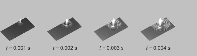
Figure 12.17 Log magnitude spectrum |U| of impulse response of a plate, with κ = 2, and of aspect ratio 2, over different frequency ranges, as indicated.

One may show, as in the case of the wave equation, that for a plate of stiffness parameter κ, and of surface area A, that the amount of memory required will be approximately

12.29

which, for typical plate materials and geometries (κ = 0.737, A = 2), and at an audio sample rate such as 48 kHz, is not particularly large (here, for a finite difference scheme, N = 8.29 × 104). The dependence of memory requirements may be directly related to both the dispersive character of the plate, as well as the constancy of mode density [Bil09]. The operation count will again scale with N · fs—which, in comparison with full 3D modeling, is in the Gflop range, which is expensive still by today's standards, but not unreasonably so. As such, it is worth looking at how one might design such a simulation through the direct time/space solution of the plate equation.

Case Study: Finite Difference Plate Reverberation

The emulation of distributed models, such as plates or springs, requires a different treatment from lumped analog components—probably the best-known distributed modeling techniques in sound synthesis are digital waveguides [Smi10], which are extremely efficient for problems in 1D, but for which such an efficiency advantage does not extend to problems in higher dimensions. Mainstream time-domain numerical simulation techniques (of which finite difference schemes [Str89] are the easiest to understand, and simplest to program) are an attractive alternative. Here, a very simple time-domain finite-difference scheme [Str89] will be presented, based on the direct solution to the equation of motion (12.25) for a thin plate. Finite difference schemes for plates are discussed by various authors (see, e.g., [Szi74]), and have been used in musical acoustics applications [LCM01], as well as in the present case of plate reverberation [Arc08, BAC06, Bil07].

Equation (12.25) describes free vibration of a lossless thin plate. A simple extension to the more realistic case of frequency-independent loss, and where the plate is driven externally (as in a reverberation unit) is

12.30

Here σ ≥ 0 is a loss parameter—it is related to a global T60 reverberation time by T60 = 6ln(10)/σ. More realistic (frequency-dependent) models of loss are available [CL01], but the above is sufficient for a simple demonstration of finite difference techniques. f(t) is a force signal in N, assumed known, and applied at the location x = xi, y = yi, where here, δ is a Dirac delta function.

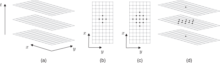
The first step in the design of any audio effect is the choice of a sample rate fs. In simulation applications, it is more natural to make use of a time step T = 1/fs. Another choice which must be made is that of a spatial grid, at the points of which an approximate solution to a partial differential equation will be computed. In the case of a plate defined over a rectangular domain x ∈ [0, Lx], and y ∈ [0, Ly], the obvious choice is a rectangular grid, of spacing X between adjacent points. The grid function then represents an approximation to the solution u(x, y, t) of (12.25), at times t = nT, and at locations x = lX, and y = mX, for integer n, l and m. See Figure 12.18(a). It makes sense to choose X such that the grid spacing divides the side lengths as evenly as possible, i.e., , for some integers Nx and Ny. It is not possible to do this exactly for arbitrary side lengths—to remedy this, one could choose distinct grid spacings X and Y in the x and y directions, but this subtle point will not be explored further here. There are, of course, many other ways of choosing grids, which may or may not be regular—finite element methods [Coo02], for example, are usually designed to operate over unstructured grids, and are suitable for problems in irregular geometries. Consider first the first and second partial time derivatives which appear in (12.25). The simplest finite-difference approximations, δt and δtt may be written as

12.31

12.32

The other operation which must be approximated is the Laplacian ∇2, as defined in (12.26). Here is the simplest (five-point) choice,

12.33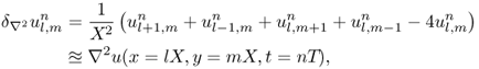

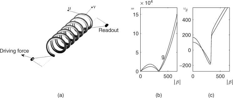
see Figure 12.18(b). System (12.30) requires a double application of this operator—see Figure 12.18(c). Near the edges of the domain, this operation appears to require values which lie beyond the edges of the grid—these may be set by applying the appropriate boundary conditions. For a plate reverberation unit, these will be of free type, but in the MATLAB example which follows, for simplicity, they have been set to be of a simply supported type (i.e., the plate is constrained at its edges, but able to pivot). A complete treatment of numerical boundary conditions is beyond the scope of the present chapter—see [Bil09] for more information.

Figure 12.18 (a) Computational grid, defined over Cartesian coordinates x and y, and for time t. (b) Computational footprint of the five-point Laplacian operator, and (c) when applied twice. (d) Computational footprint for the scheme (12.34).

A complete scheme for (12.25) then follows as

12.34

This scheme relies on a discrete delta function , picking out a grid location corresponding to x = xi, and y = yi (perhaps through truncation), and a sampled input signal fn. The scheme operates over three time levels, or steps, as shown in (d), and is also explicit—values at the unknown time step n + 1 may be written in terms of previously computed values (after expanding out the operator notation above) as

12.35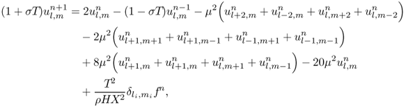

where μ = κT/X2 is a numerical parameter for the scheme. It may be shown that for stability, one must choose

12.36

and in fact, in order to reduce artifacts due to numerical dispersion (i.e., additional unwanted dispersive behavior induced by the scheme itself, on top of that inherent to the plate itself), this bound should be satisfied as near to equality as possible. In audio applications, this allows the grid spacing X to be chosen in terms of the sample rate. See [Bil09] for much more on the properties of this scheme.

In implementation, it can be useful to rewrite this scheme in a vector-matrix form. A grid function , representing the values of a grid function over a rectangular region, may be rewritten as a column vector un, consisting of consecutive “stacked” columns of values over the grid, at time step n. Because the scheme as a whole is linear, and explicit, it must then be possible to rewrite it as the two-step recursion,

12.37

Here, the effects of loss and the spatial difference operators have been consolidated in the (extremely sparse) matrices B and C, and r is a column vector which chooses an input location. Output may be drawn from the scheme at a location x = xo, y = yo by simply reading at each time step. In vector form, the output yn may be written as

12.38

for some vector q, which, in the simplest case, will consist of a single value at the readout location.

Below is a very simple MATLAB implementation of the plate reverberation algorithm mentioned above—it generates a reverberant output, for a given plate, sample rate, and excitation and readout points. It's not particularly fast (at least in MATLAB)—but not extremely slow either!

This example is written to be compact and readable—and many more realistic features which have been omitted could be added in. Among these are:

• Frequency-dependent damping—at the moment the T60 is set to be uniform at all frequencies. This could be done directly in the PDE model above, or possibly through introducing a model of a damping plate.
• Boundary conditions are set to be simply supported—allowing the easy generation of difference matrices. These should ideally be set to be free, or going further, to incorporate the effect of point supports.
• Only a single output is generated—multiple outputs (such as stereo, but perhaps more in a virtual environment) should be allowed. Notice that multiple outputs may be generated essentially “for free,” as the entire state (u) is available.
• Output displacement is taken; in real plate reverberation units, it is rather an acceleration—acceleration can be derived from displacement easily through a double time difference operation.
• Post-processing (analog electronic) and the behavior of the pickup are not modelled.

Information on all these extensions appears in various publications, including those mentioned at the beginning of this section.

12.4.3 Springs and Spring Reverberation

A helical spring under low tension has long been used as an artificial reverberation device [Ham41, YI63, Sta48]. In most units, the spring is driven through an electromagnetic coupling at one end, and readout is taken via a pickup at the opposite end. Spring reverbs come in a variety of sizes and configurations, sometimes involving multiple springs. A typical set-up is shown in Figure 12.19(a).

Figure 12.19 (a) A typical spring reverberation configuration, for a spring driven at one end, and with readout taken from the other; longitudinal and transverse motion of the spring are indicated by u and v. (b) Dispersion relations ω(β), and (c) group velocities vg(β).

The physics of helical structures is far more involved than that of the flat plate—see [Wit66, DdV82] for typical models. The important point is that the various types of motion (transverse to the spring, in both polarizations, and longitudinal) are strongly coupled in a way that they are not for a straight wire. A complex combination of relatively coherent wave propagation (leading to echoes) and highly dispersive propagation is present, leading to a characteristic sound which resembles both real room responses, and plate reverbs.

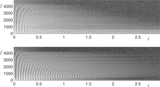
One can garner much useful information from the dispersion relations for a spring, as shown in Figure 12.19(b). For springs of dimensions and composition as found in reverberation devices, there are two relations which lie within the audio range—both correspond to mixtures (wavenumber-dependent!) of longitudinal and transverse motion. Both curves exhibit a “hump” in the low wavenumber range corresponding to a cutoff—for most spring reverb units, this occurs in the range between 2 kHz and 5 kHz. An examination of the group velocities, as shown in Figure 12.19(c) allows for some insight with regard to the behavior of spring responses, an example of which is shown at top in Figure 12.20. In the range of low wavenumbers, the group velocities approach a constant value, and thus dispersion is low at low frequencies, and strong echoes are present. But as the wavenumber increases towards the cutoff, the group velocity decreases, and thus the frequency components of the echoes are distorted increasingly (slowed) near the cutoff. Above the cutoff, the group velocity is much faster, and leads to distorted echoes which recur at a higher rate. Above the cutoff, the response is very similar to transverse motion for a straight bar.

Figure 12.20 Top, spectrogram of a measured spring reverberation response, and bottom, that of a synthetic response produced using a finite difference model.

Emulation Techniques

As in the case of plate reverberation, there is a variety of techniques available—and as of 2010, physical modeling of springs is still an open research problem. The most rigorous approach, given a partial differential equation model, is again a time-stepping method such as finite differences, which has been used by this author [Bil09, BP10], as well as Parker [Par08] in order to generate synthetic responses. See Figure 12.20(b) for a comparison between a measured response and synthetic output. This approach turns out to be rather expensive, and given that the system is essentially 1D (i.e., for a thin spring, the equations of motion may be written with respect to a single coordinate running along the spring helix), structures based on delay lines and allpass networks are a possibility, and an excellent compromise between physical and perceptual modeling. See, e.g., [ABCS] and [VPA10].

The difficulties here lie in associating such a model with an underlying model in a definitive way. Another approach, as yet unexplored, could be based on the use of a modal decomposition. In other words, given appropriate boundary conditions, one may solve for the modes of vibration of the helix. This is the approach taken in the analysis of helical structures in mainstream applications—see, e.g., [LT01].