
Field orientation, VA requirement and magnetic saturation
In this chapter some further fundamental aspects of the bearingless motor are discussed. The first point concerns the misalignment of the revolving magnetic field. A phase shift between the detected and actual field orientation produces interference in the two-axis radial force generation which causes operational discrepancies and hence stability problems in the radial position regulation loops. The phase shift may occur if the suspension force constants are not precise and accurate. These constants may vary depending on torque and suspension force outputs. The influence and measurement of the suspension force misalignment are therefore introduced.
In the second section an example is shown for the voltage and current (VA) requirement at the suspension winding terminals. For efficient operation and maximization of capacity, the required VA should be as low as possible. The requirement is dependent on the required suspension force and the radial sensor signal conditions. Since both motor and suspension voltages are proportional to the rotational speed, the suspension winding VA requirement is also expressed as a ratio with respect to the motor winding VA requirement.
In the final section the influence of magnetic saturation on the suspension force generation is discussed. A relationship between the suspension force, the current and the tooth flux density is shown for a primitive bearingless motor so that an operating point can be suggested.
8.1 Misalignment of field orientation
Figure 8.1(a,b) shows the principles of radial force interference between the x and y axes when the angular position of the revolving magnetic field has a phase lag angle of θ. Figure 8.1(a) shows the radial force generation without interference. The ma winding flux indicates the equivalent current directions for the revolving magnetic field Ψma, which has a 4-pole distribution. For suspension, positive current in winding sa generates a 2-pole flux Ψsa. In air-gap section 1 the directions of Ψma and Ψsa are the same whereas they are opposite in air-gap section 3 so that radial force is generated along the x-axis.
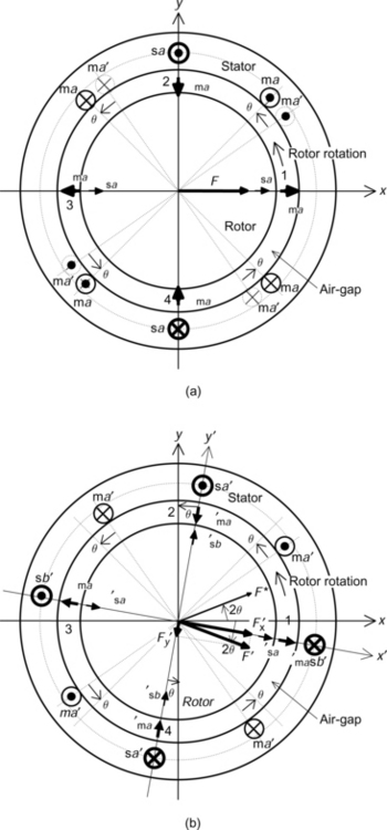
Figure 8.1 The variations in the radial force direction depending on the 4-pole flux orientation: (a) exact field flux orientation; (b) the 4-pole flux with a phase lag angle θ
Let us suppose that the 4-pole excitation current is delayed by an electrical angle of 2θ so that the 4-pole revolving magnetic field is delayed by a mechanical angle θ with respect to the x–y coordinates. Winding ma′, shown by the dotted line in Figure 8.1(a), indicates the position of the equivalent winding for a 4-pole magnetic field with the lag angle of θ. New x′- and y′-axes are drawn in Figure 8.1(b), which are rotated by θ and correspond to the rotation of the 4-pole magnetic field. Let us examine the case when a suspension current exists only in winding sa. This can be represented by two equivalent current components in the sa′- and sb′-windings, which are on the x′- and y′-axes. With current in winding sa′, a flux Ψ′sa is generated and the interaction with the 4-pole flux Ψ′ma generates a radial force of F′x. When there is current in winding sb′, a 2-pole flux Ψ′sb is generated which results in a radial force of F′y. The resulting radial force F′ is a vector sum of these two radial forces and has a direction which is delayed by an angle 2θ. Hence if interference occurs in the radial forces in two perpendicular axes, the response of the radial positioning loops becomes worse. A basic example was discussed previously in section 3.3. More examples of the practical implementation of the bearingless motor concept which highlight this sort of alignment issue are discussed in this section.
Figure 8.2 shows a method to check the radial force interference under steady-state conditions [1]. An external static radial force Fex is applied to a rotating shaft. The amplitude and direction of the external radial force are fixed. This can be implemented by using a weight hanging from a thread on a pulley with the other end fixed to a mechanical bearing on the rotating shaft. In addition, with a horizontal shaft arrangement, the shaft and rotor weight acts as an external static force so that the shaft arrangement has to be suspended by magnetic force with radial position feedback loops. If the motor magnetic field corresponds to the sine and cosine components in the modulation block then the radial force command F*x is generated which has the same amplitude but opposite direction to the external force so that the net force Fx is zero.
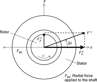
However, the radial force commands are automatically varied if there is a misalignment in angular position detection of the motor magnetic field. If the mechanical phase lag angle is θ then a radial force command F* is generated with a phase lead of 2θ so that the generated radial force is exactly opposite in order to satisfy the force equilibrium. We can check the misalignment of the revolving motor magnetic field detection by observing the radial forces which are generated by the radial position controllers.
Figure 8.3 shows an example of the phase-shift angle for an induction-type bearingless motor. At slip = 0, the phase shift angle is almost zero, i.e., the line current and revolving magnetic field almost correspond. For example, the u-phase line current indicates a cosine component of flux linkage when the u-phase MMF and the x-axis are aligned. As the rotor slip is increased, the revolving magnetic field is delayed with respect to the line current (as would be expected in an induction motor). The amplitude of the revolving magnetic field also decreases when the current amplitude is kept constant. In the following examples, a field-oriented controller and a constant current controller are employed to see phase-shift influence.

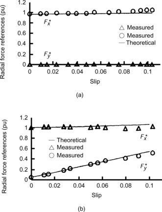
Figure 8.4 shows the measured radial force references as a function of rotor slip for two cases. The first is with exact field orientation and the second is with the misalignment as shown in the previous figure. An external radial force is applied along the negative x-axis. In Figure 8.4(a), F*x and F*y are unity and zero respectively. In Figure 8.4(b), F*y increases as the slip increases and the revolving magnetic field is delayed with respect to the cosine and sine components of modulation. Since there is a negative phase shift in motor field orientation a positive F*y is generated automatically. At slip = 0.1, F*y = 0.48 and F*x = 1, which correspond to 2θ = 26 deg. This angle corresponds to the phase shift angle shown in Figure 8.3.
There are some practical points that can be checked during the measurement of the radial force references. The radial position loops may become unstable if the misalignment is too large so that the controller parameters in the radial position loops should be adjusted to allow for the phase shift angle. In some cases, decreasing the loop gains will provide some margin.
During measurements, the shaft is suspended by a magnetic force so that waveforms are produced from the radial force references. These include fluctuations caused by sensor noise, unbalance and mechanical misalignments. The applied external radial force may have synchronous variations caused by synchronous shaft displacements. Hence the ac component should be eliminated by a low pass filter to detect only the dc components.
Figure 8.5 shows a comparison of step disturbance suppression in the radial position loops. A step disturbance signal is added to the output of the x-axis radial-position PID controller while the shaft is rotating at constant speed and suspended by a magnetic force. Hence the influence of the step disturbance results in x-axis shaft radial displacement so that the radial position controllers automatically generate a radial force reference F*x to suppress the disturbance signal. Because the speed of this process is determined by the rotor shaft inertia, there is a delay of several milliseconds. Figure 8.5(a,b) shows the behaviour of the disturbance signal Fxd, displacement y and radial force references F*y and F*x. The radial force reference F*x is the output signal from the step signal summation as shown in Figure 8.5(c). In Figure 8.5(a) the influence of step disturbance is seen in only F*x because of the exact field orientation. After the transient response, F*x decreases to cancel the step disturbance.
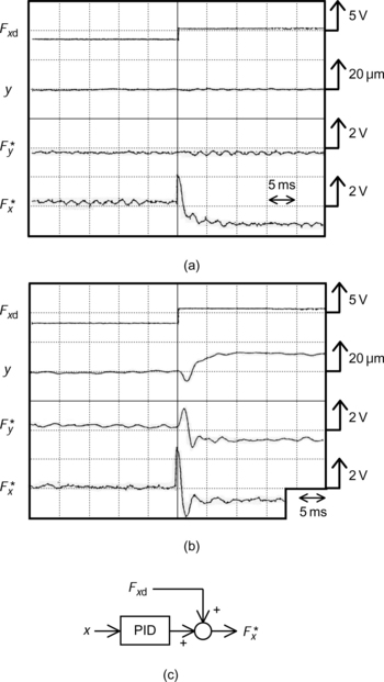
Figure 8.5 Step disturbance force suppression: (a) exact field orientation; (b) misalignment in magnetic field; (c) step disturbance summation
In Figure 8.5(b) the influence of the x-axis step disturbance is seen in the y-axis variables. A misalignment of field orientation generates radial force on the y-axis, hence the radial positioning loop automatically generates a signal F*y to suppress the disturbance. The radial displacement y cannot be totally suppressed. In addition, more vibration is seen in the response of F*x because of the inferior feedback loop characteristics caused by coupling between the two perpendicular axes (as previously shown in section 3.3).
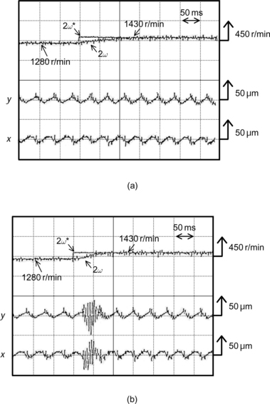
Figure 8.6(a,b) shows a comparison of the waveforms during a small step in acceleration. The shaft speed command 2ω* is increased from 1280 to 1430r/min as a step function. To follow the speed command the torque current increases to the maximum value so that the speed ramps up at a rate determined by the mechanical inertia. With an exact field orientation the influence of acceleration is not seen in radial displacements x and y. However, significant fluctuations are seen if there is a misalignment in field orientation. The misalignment angle appears just after the step change in the speed command so that it decreases as the shaft speed 2ω approaches the speed command. The misalignment angle is zero when shaft speed is following the speed command. Fluctuations in radial displacements are seen just after the maximum misalignment angle occurs (although misalignment angle is not shown here), which is during torque generation for the induction type of bearingless motor. The misalignment of the actual magnetic field components, and the modulating cosine and sine functions, should be minimized to prevent high radial disturbance.
8.2 VA requirement
In magnetic suspension, regulated ac current should be supplied to the suspension windings. These induce winding back-EMFs which are proportional to the winding inductance and supply frequency. To produce successful current regulation the rated voltage of the supply inverter must be larger than the induced EMFs. The product of the terminal voltage and line current is called the VA (unit: [volt-ampere]) requirement.
If the number of series turns N of a winding is increased then the required current needed to produce the same MMF decreases by 1/N. However, the induced terminal voltage increases by N since the inductance increases by N2. Hence the product of voltage and current is not a function of the number of winding turns although the VA requirement is found to be a unique value.
In this section the voltage and current requirements at the suspension winding terminals are derived, for example, for the induction-type bearingless motor. The required voltage and current for static radial force is derived and it is found that the VA requirement is proportional to the rotational speed. It is also shown that the no-load VA requirement at the motor winding terminals for motor operation magnetization is also proportional to rotational speed so that the ratio of these VA requirements is independent of speed. The VA ratio provides a simple index for a bearingless motor. In the following discussion of an induction type of bearingless motor, the VA requirement, its ratio and the power ratio are addressed. Finally the VA and efficiency definition for a permanent magnet bearingless motor is also described for completeness.
8.2.1 Induction-type bearingless motor
Let us suppose that a 3-phase 4-pole winding is the motor winding and a 3-phase 2-pole winding is the suspension winding. The rms value of a 3-phase line current in the 4-pole winding is Im and the rms line-to-line voltage at the motor winding terminals Vml is
where ω is the mechanical angular speed of the shaft at no torque (synchronous speed) so that the current frequency is equal to 2 ω (since it is a 4-pole winding). This assumes no rotor current. The total voltage and current requirement VAm at the motor winding terminals is a product of the line-to-line voltage and current for all three phases and can be written as (assuming a balanced 3-phase set):
Substituting (8.1) into (8.2) yields
To produce a static radial force F the rms line current in the suspension windings Is is
and has a frequency of 2ω. The line-to-line voltage Vsl at the suspension winding terminals is therefore
so that the total VA requirement of the 2-pole winding for 3-phases is written as
Substituting (8.5) into (8.6) yields
Note that the VA requirements in (8.3) and (8.7) are proportional to the speed. Hence the ratio of the VA requirements is
The VA ratio is a function of the inductances, motor exciting current and required suspension current. This ratio provides a simple index for the voltage and current requirements of the suspension inverter. For example, if the ratio is 0.01 then a motor excitation of 2 kVA requires a suspension inverter of 20VA.
Figure 8.7 shows the measured rms values of line current and line-to-line voltage at the motor winding terminals. Over the whole speed range the line current is constant, providing reasonable excitation. The voltage is proportional to the rotational speed. Since the test machine is driven by a PWM inverter, the rms value is slightly more than the fundamental component, which has an angular frequency of 2ω (where ω is the rotational speed in rad/sec at no load). The fundamental component corresponds to the theoretical values.
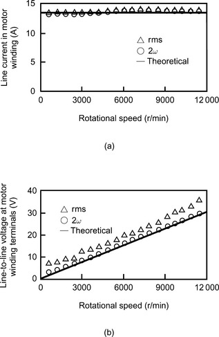
Figure 8.8 shows waveforms for the line current imu and line-to-line voltage νmuv at a speed of 10 200r/min. The current waveforms include the switching ripple caused by the PWM output voltage of the voltage-source inverter. Surge voltages are also seen at the switching instances.
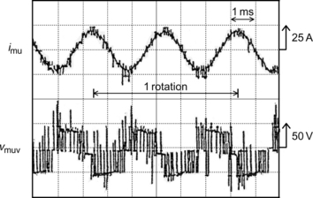
Figure 8.9 shows the rms current and voltage for the suspension winding. The current has several harmonic components in addition to the 2ω component necessary to produce the static suspension force. The major additional component has a frequency of ω which is dependent on the rotational speed and is maximum at the critical speed of 6000 r/min. This is because the vibration caused by mechanical unbalance is suppressed by the suspension winding current of this frequency. On the other hand the 2ω frequency component is almost constant since the static radial force is constant at 2.6 kgf across the whole speed range. In the voltage waveform the 2ω component is dominant and the voltage is proportional to the rotational speed, as expected.
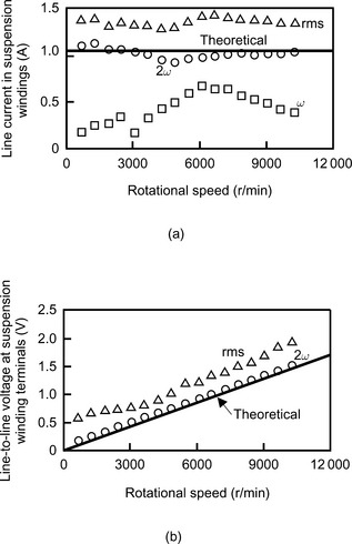
Figure 8.9 Current and voltage of suspension winding terminals with static force of 2.6 kgf: (a) line current; (b) line-to-line voltage
Figure 8.10 shows the current and voltage waveforms for the suspension winding when a static force of 2.6 kgf is applied at a speed of 10 200 r/min. It can be observed that the 2ω voltage and current components are dominant even when the radial force suspension current is driven by a PWM inverter.
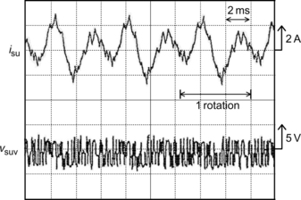
Table 8.1 shows a summary of the voltages, currents and VAs for the motor and suspension windings of the induction-type bearingless motor example. The rms values are measured by digital power meters that have a wide frequency range and the fundamental components are obtained by an FFT (fast Fourier transform) analyser. The measured (total rms and 2ω components) and theoretical values are shown for comparison. The measured VA ratio of the fundamental component is 0.0043 which is close to the theoretical value of 0.0039. The measured rms VA ratio is 0.0059, which is slightly high. The reasons for this discrepancy can be summarized as follows:
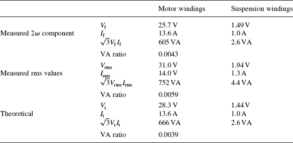
(a) The measured rms current includes a current component to suppress the mechanical unbalance. This has an angular frequency of ω.
(b) The measured rms current includes high frequency components caused by sensor noise.
The example shown in this section is based on Reference [2]. For the test induction type of bearingless motor the VA ratio is quite low when compared to its shaft weight of 2.6 kg. The VA ratio increases as the required radial force increases. If a ninefold increase in the radial force is required in this machine then the VA ratio increases by 81 times (since it is a square relationship).
Several other machines have been tested. Experience suggests that there are several key issues that have to be addressed to obtain performance figures that are close to the theoretical. These are:
8.2.2 Permanent magnet type bearingless motor
An example of an inset permanent magnet bearingless motor is described in this section. In PM machines the motor winding terminal VA is zero at no-load (since there is no motor winding current, the excitation is via magnets). Hence the VA ratio has to be determined using the maximum rated torque VA requirement.
Table 8.2 shows the result of a load test at 10000r/min [3]. The voltage and current ratings of the motor winding terminals are 150V and 11.1 A respectively. The input and shaft powers are 2.23, 2.06 kW. At the suspension winding terminals the current, voltage and power are 3.95A, 39.3V and 25.7W. These values are required to suppress the synchronous disturbance caused by the mechanical shaft unbalance, the misalignment of shaft parts, sensor noise and so on. The VA ratio at the rated maximum torque point is 0.09. This VA ratio is reasonably low. Further reduction is possible by improvement of the mechanical precision and sensor signal conditions; however, this adds additional cost.
Table 8.2
Load test results of an inset permanent magnet bearingless motor
| Rotational speed | 10 000 r/min |
| Motor winding | |
| Line current Im | 11.1A |
| Line-to-line voltage Vml | 150V |
| Input VA, VAm | 2.88 kVA |
| Input power Pm | 2.23 kW |
| Copper loss | 95.2 W |
| Iron loss + other loss | 75.0 W |
| Output power Po | 2.06 kW |
| Efficiency Po/Pm | 92.4% |
| Suspension winding | |
| Line current Is | 3.95A |
| Line-to-line voltages Vsl | 39.3 V |
| Input VA, VAs | 269 VA |
| Input power Ps | 25.7W |
| VA ratio | 0.09 |
| Efficiency Po/(Pm + Ps) | 91.3% |
8.3 Magnetic saturation
In this section the effect of magnetic steel saturation on the suspension force is discussed [4]. Results from the finite element analysis of a primitive bearingless machine are shown and an operating point is suggested. The concept of radial force density is then introduced.
Figure 8.11(a–c) shows flux plots for a primitive bearingless motor with suspension winding currents of I2 = 0.8, 1.2 and 2.5 A. The cases for I2 = 0 and 0.5 A were previously shown in Figure 6.3. At I2 = 0 the flux distribution is symmetrical. As I2 increases the 2-pole flux is superimposed. In Figure 8.11(a) the tooth flux density B_ is almost zero. In Figure 8.11(b) the radial force reaches the maximum value and after this point the radial force decreases as shown in Figure 8.11(c).
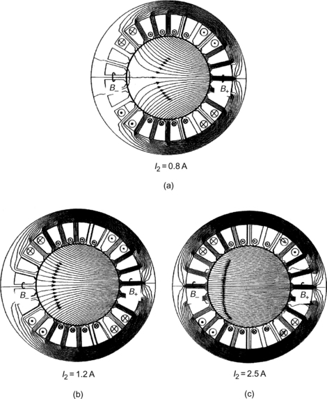
Figure 8.11 Flux plots: (a) B− is approximately zero; (b) radial force is maximum; (c) radial force is decreased
Figure 8.12 shows the variation of calculated tooth flux density. The current conditions a to e are for the flux plots in Figures 6.3(a,b) and 8.11(a–c) respectively. In addition, the measured flux densities in a test machine are shown. The flux densities B+ and B− are the same at I2 = 0. Then B+ increases, and the influence of magnetic saturation is seen as the maximum is reached. For silicon steel, which is used in almost all motors and generators, the saturated flux density is about 1.7 to 2.0 T. On the other hand, B− keeps decreasing and becomes zero at around I2 = 0.8 A. After this point B− becomes negative and further decreases until saturation sets in and B− = −B+. Since the magnetic force is always attractive and is almost proportional to the square of airgap flux density, the effect of saturation on the radial force occurs from the operating point c; and by the time point e is reached, saturation has caused the airgap flux to become more evenly distributed, and hence the radial force to decrease.
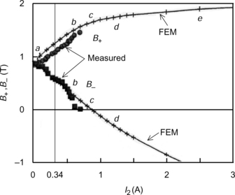
Figure 8.13 shows the relationship between the radial force and suspension winding current. As illustrated by the finite element method (FEM) analysis, the radial force is maximum at point d, then it decreases as the steel saturation further increases. The derivative (slope) of the curve gradually decreases from around point c where saturation first occurs. Experiments were possible only up to just before point c because of a decrease in loop gain. It may be possible to operate further into the saturated region if a nonlinear controller is used to compensate radial force saturation.
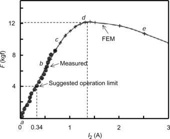
A suggested operation limit point is about 4kgf. One may feel that this operation point is too low for radial force generation. However, there are some merits to operation in the region between point a and this suggested point:
(a) Good linearity is obtained in the relationship between radial force and current.
(b) Flux density variation in the teeth is about 0.25 T for B+ and B−, which should not greatly affect the performance of the motor-drive characteristics.
In the case of a highly saturated electric machine, such as those used in aerospace applications, (b) may not apply. However, in most industrial applications there is some room for small flux variations.
The example shown in this section is based on specific dimensions. The rotor diameter D is 49 mm with an axial length l of 30.8 mm so that the rotor shadow area Dl is about 15 cm2. A 4 kgf radial force has a radial force density of about 0.3 kgf/cm2. This value may appear low compared to a radial magnetic bearing which has a practical radial force density of 1 kgf/cm2. However, the area is usually much larger in a bearingless motor compared to a magnetic bearing, because the motor and magnetic bearing are combined, so that the suggested radial force density is acceptable in most cases.
References
[1] Chiba, A., Furuichi, R., Aikawa, Y., Shimada, K., Takamoto, Y., Fukao, T., “Stable Operation of Induction-Type Bearingless Motors Under Loaded Conditions”. IEEE Trans. on IAS, Vol. 33, No. 4, 1997:919–924. [July].
[2] Ito, E., Chiba, A., Fukao, T., “A Measurement of VA Requirement in an Induction-type Bearingless Motor”. IV International Symposium on Magnetic Suspension Technology, Gifu-Japan, 1998:125–137. [May].
[3] Inagaki, K., Chiba, A., Rahman, M.A., Fukao, T., “Performance Characteristics of Inset-Type Permanent Magnet Bearingless Motor Drives”. IEEE PES, WMC, CDROM Singapore, 2000. [January].
[4] Chiba, A., Fukao, T., “The Maximum Radial Force of Induction Machine-Type Bearingless Motor Using Finite Element Analysis”. ISMB, 1994:333–338. [August].