
Controllers and power electronics
In this chapter, a digital controller and a sample program for controlling a bearingless motor are introduced. This is a general-purpose structure that can be modified and tailored to a specific bearingless drive application.
19.1 Structure of digital controllers
Currently, digital control using digital signal processors (DSP) is usually used in a bearingless drive to realize the system. This is because:
1. The drive inverters generate a lot of electromagnetic noise due to switching. However, the interference caused by this noise in the control loop of the magnetic suspension can be reduced by using digital control. In particular, digital control can protect the delicate derivative controller, which is essential for magnetic suspension.
2. Digital control allows a higher degree of flexibility and universality compared with analogue control.
3. When using analogue control, it is difficult to introduce complex control methods such as an observer, a nonlinear calculation (such as magnetic saturation) or any calculation using complex branching methods or extensive memory. However, digital control can deal with these complex control methods.
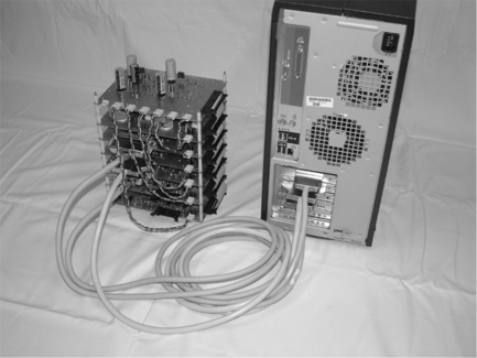
Figure 19.1 shows the typical structure of a digital control system in a bearingless drive using hysteresis current regulators. An example of a complete digital control system is illustrated in Figure 19.2.
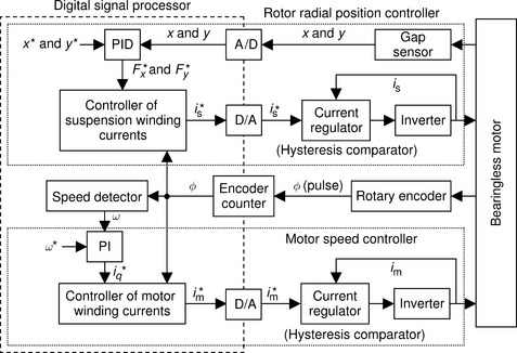
Figure 19.1 Typical structure of a digital control system in a bearingless drive using hysteresis comparators
In the motor speed controller the rotor angular position φ is detected by the rotary encoder. The rotational speed ω is generated from the encoder counter and speed detector. This is then compared to the rotational speed command ω*, and the q-axis current command i*q (in rotating angular coordinate) is generated by the proportional-integral (PI) controller which is applied to the speed error. In the motor winding current controller, the 3-phase motor winding current command i*m is calculated by transforming i*q from the rotating angular coordinate to the stationary coordinate and transforming from 2-phase to 3-phase. Finally, the motor winding currents are controlled by the current regulator using hysteresis comparators and the 3-phase inverter.
In the rotor radial position controller, the rotor displacements x and y (on the x and y axes) are detected by the gap sensors through an A/D converter and these displacements are compared to the displacement commands x* and y*. The suspension force commands F*x and F*y are generated by the proportional-integral-derivative (PID) controllers. The outputs are then fed into the suspension winding current controller where F*x and F*y are modulated to become the 2-phase suspension winding current commands by means of sinusoidal functions which are synchronized to the rotor angular position φ. These 2-phase commands are then transformed into 3-phase commands. The controller for the suspension winding currents has been discussed in each chapter as the various bearingless motors were introduced. The 3-phase suspension winding current command i*s is fed forward to the current regulator via the D/A converter where the suspension winding currents are generated by the hysteresis comparators in the regulator and the 3-phase inverter. As an example, Figure 19.2 shows a digital controller complete with current regulators, power supply and analogue interface circuits fabricated on layered printed boards.
An alternative current regulation scheme for the regulator can be realized in rotating coordinates instead of by the hysteresis method. The detected currents are transformed into the rotating reference frame coordinates and then compared with rotating current references. The current errors are amplified by PI controllers to generate voltage references, and gate pulses are generated by comparison of the voltage references with triangular carrier waveforms.
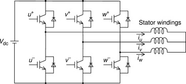
The current regulator, consisting of the hysteresis current regulators and inverter drive, was explained in detail in Chapter 5. Figure 19.3 shows the main circuit of a 3-phase inverter suitable for use in a bearingless drive. This is made up of six power-switching devices, such as IGBTs, MOSFETs, transistors, etc., each encapsulated with an anti-parallel diode.
19.2 Discrete-time systems of PID controllers with the z-transform
It is necessary to transform the PID controllers from continuous-time operation to discrete-time operation in order to construct the rotor radial position controller using a digital controller as shown in Figure 19.1. For this purpose, the z-transform is used. In this section, the discrete-time operation of the PID controller in the z-domain, as well as a sample program for realizing the controller, are introduced.
19.2.1 A PID controller in the z-domain
Figure 19.4(a) shows the block diagram of an ideal PID controller in the s-domain. Kp, Ki and Kd are the gain coefficients of the proportional, integral and derivative components of the controller respectively, while s(t) and x(t) are the input and output signals in the continuous-time domain. The transfer function of the PID controller in Figure 19.4(a) can be expressed as
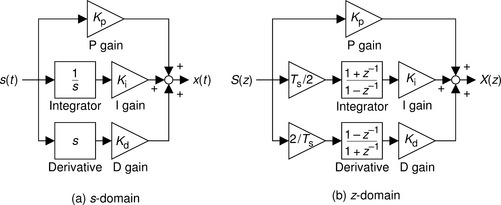
The transfer function of the PID controller in the z-domain can be derived by applying the z-transform to (19.1) so that
where Ts is the sampling period. Figure 19.4(b) shows a block diagram of the PID controller in the z-domain and S(z) and X(z) are the input and output signals respectively in the discrete-time domain.
19.2.2 A sample program of a PID controller
The transfer function of the integral controller can be re-written from (19.2) as
where Si(z) and Xi(z) are the input and output signals of the integral controller. To understand the basic operation of the integral controller in the z-domain, the controller is illustrated in a block diagram form using (19.3) as shown in Figure 19.5(a). This block diagram can be transformed into the block diagram shown in Figure 19.5(b) where Wi(0) and Wi(1) are medium factors of the integrator.
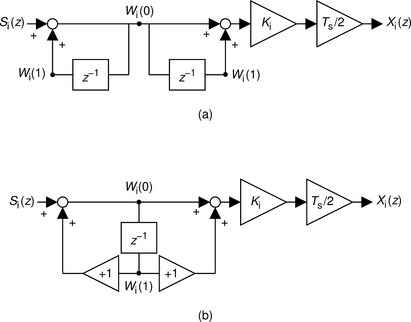
Figure 19.5 Block diagrams of the integral controller: (a) the block diagram of the integral controller based on (19.3) (b) the general block diagram of the integral controller
From Figure 19.5 the following expressions can be derived
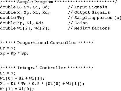
An outline of the programming required for the integral controller in the discrete-time domain is listed below and it is derived from (19.4), (19.5), and (19.6).
Similarly, the derivative controller in the z-domain is illustrated in a block diagram form in Figure 19.6. The variable definitions in Figure 19.6 are as follows: Wd (0) and Wd (1) are medium factors of the derivative, Sd(z) is the input signal and Xd(z) is the output signal.
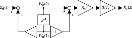
The following expressions can be obtained from Figure 19.6:
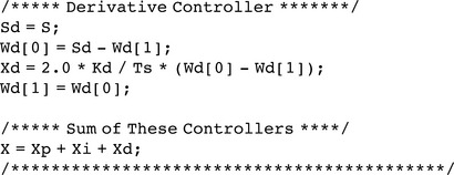
Again, an outline program for the derivative controller in the discrete-time domain, as obtained from (19.7), (19.8), and (19.9), is listed below.
A sample program of the PID controller in C-language is:
The other components of the digital controller program are straightforward because the modulation, coordinate transformation, 2-phase to 3-phase conversion and nonlinear parameter variations are simple calculations using the inputs at the start of the sample period.