
PART III: PROBLEMS
Section 8.1
8.1.1 Let ![]() = {B(N, θ);0 < θ < 1} be the family of binomial distributions.
= {B(N, θ);0 < θ < 1} be the family of binomial distributions.
8.1.2 Let X1, …, Xn be i.i.d. random variables having a Pareto distribution, with p.d.f.
![]()
0 < ν < ∞ (A is a specified positive constant).
 , is a minimal sufficient statistic.
8.1.3 Let X be a p–dimensional vector having a multinormal distribution N(μ, ![]() ). Suppose that
). Suppose that ![]() is known and that μ has a prior normal distribution N(μ0, V). What is the posterior distribution of μ given X?
is known and that μ has a prior normal distribution N(μ0, V). What is the posterior distribution of μ given X?
8.1.4 Apply the results of Problem 3 to determine the posterior distribution of β in the normal multiple regression model of full rank, when σ2 is known. More specifically, let
![]()
8.1.5 Let X1, …, Xn be i.i.d. random variables having a Poisson distribution, P(λ), 0 < λ < ∞. Compute the posterior probability P{λ ≥ ![]() n | Xn} corresponding to the Jeffreys prior.
n | Xn} corresponding to the Jeffreys prior.
8.1.6 Suppose that X1, …, Xn are i.i.d. random variables having a N(0, σ2) distribution, 0 < σ2 < ∞.
8.1.7 Let X1, …, Xn be i.i.d. random variables having a N(μ, σ2) distribution; −∞ < μ < ∞, 0 < σ < ∞. A normal–inverted gamma prior distribution for μ, σ2 assumes that the conditional prior distribution of μ, given σ2, is N(μ0, λ σ2) and that the prior distribution of 1/2σ2 is a ![]() . Derive the posterior joint distribution of (μ, σ2) given (
. Derive the posterior joint distribution of (μ, σ2) given (![]() , S2), where
, S2), where ![]() and S2 are the sample mean and variance, respectively.
and S2 are the sample mean and variance, respectively.
8.1.8 Consider again Problem 7 assuming that μ and σ2 are priorly independent, with μ ∼ N(μ0, D2) and ![]() . What are the posterior expectations and variances of μ and of σ2, given (
. What are the posterior expectations and variances of μ and of σ2, given (![]() , S2)?
, S2)?
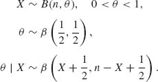
8.1.9 Let X ∼ B(n, θ), 0 < θ < 1. Suppose that θ has a prior beta distribution ![]() . Suppose that the loss function associated with estimating θ by
. Suppose that the loss function associated with estimating θ by ![]() is L(θ,
is L(θ, ![]() ). Find the risk function and the posterior risk when L(
). Find the risk function and the posterior risk when L(![]() , θ) is
, θ) is
8.1.10 Consider a decision problem in which θ can assume the values in the set {θ0, θ1}. If i.i.d. random variables X1, …, Xn are observed, their joint p.d.f. is f(xn;θ) where θ is either θ0 or θ1. The prior probability of {θ = θ0} is η. A statistician takes actions a0 or a1. The loss function associated with this decision problem is given by

8.1.11 The time till failure of an electronic equipment, T, has an exponential distribution, i.e., ![]() ; 0 < τ < ∞. The mean–time till failure, τ, has an inverted gamma prior distribution, 1/τ ∼ G(Λ, ν). Given n observations on i.i.d. failure times T1, …, Tn, the action is an estimator
; 0 < τ < ∞. The mean–time till failure, τ, has an inverted gamma prior distribution, 1/τ ∼ G(Λ, ν). Given n observations on i.i.d. failure times T1, …, Tn, the action is an estimator ![]() . The loss function is
. The loss function is ![]() . Find the posterior risk of
. Find the posterior risk of ![]() . Which estimator will minimize the posterior risk?
. Which estimator will minimize the posterior risk?
Section 8.2
8.2.1 Let X be a random variable having a Poisson distribution, P(λ). Consider the problem of testing the two simple hypotheses H0: λ = λ0 against H1: λ = λ1; 0 < λ0 < λ1 < ∞.
![]()
where [x] is the largest integer not exceeding x.
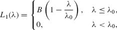
8.2.2 Let X1, …, Xn be i.i.d. random variables having an exponential distribution G(λ, 1), 0 < λ < ∞. Consider the two composite hypotheses H0: λ ≤ λ0 against H1: λ > λ0. The prior distribution of λ is ![]() . The loss functions associated with accepting Hi (i = 0, 1) are
. The loss functions associated with accepting Hi (i = 0, 1) are
![]()
and
0 < B < ∞.
8.2.3 Let X1, …, Xn be i.i.d. random variables having a binomial distribution B(1, θ). Consider the two composite hypotheses H0: θ ≤ 1/2 against H1: θ > 1/2. The prior distribution of θ is β (p, q). Compute the Bayes Factor in favor of H1 for the cases of n = 20, T = 15 and
8.2.4 Let X1, …, Xn be i.i.d. random variables having a N(μ, σ2) distribution. Let Y1, …, Ym be i.i.d. random variables having a N(η, ρ σ2) distribution, −∞ < μ, η < ∞, 0 < σ2, ρ < ∞, The X–sample is independent of the Y–sample. Consider the problem of testing the hypothesis H0: ρ ≤ 1, (μ, η, σ2) arbitrary against H1: ρ > 1, (μ, η, σ2) arbitrary. Determine the form of the Bayes test function for the formal prior p.d.f. h(μ, η, σ, ρ) ![]() and a loss function with c1 = c2 = 1.
and a loss function with c1 = c2 = 1.
8.2.5 Let X be a k–dimensional random vector having a multinomial distribution M(n;θ). We consider a Bayes test of ![]() against
against ![]() . Let θ have a prior symmetric Dirichlet distribution (8.2.27) with ν = 1 or 2 with equal hyper–prior probabilities.
. Let θ have a prior symmetric Dirichlet distribution (8.2.27) with ν = 1 or 2 with equal hyper–prior probabilities.
8.2.6 Let X1, X2, … be a sequence of i.i.d. normal random variables, N(0, σ2). Consider the problem of testing H0: σ2 = 1 against H1: σ2 = 2 sequentially. Suppose that c1 = 1 and c2 = 5, and the cost of observation is c = 0.01.
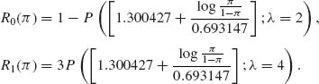
8.2.7 Let X1, X2, … be a sequence of i.i.d binomial random variables, B(1, θ), 0 < θ < 1. According to H1: θ = 0.3. According to H1: θ = 0.7. Let π, 0 < π < 1, be the prior probability of H0. Suppose that the cost for erroneous decision is b = 10[$] (either type of error) and the cost of observation is c = 0.1[$]. Derive the Bayes risk functions ρi(π), i = 1, 2, 3 and the associated decision and stopping rules of the Bayes sequential procedure.
Section 8.3
8.3.1 Let X ∼ B(n, θ) be a binomial random variable. Determine a (1 – α)–level credibility interval for θ with respect to the Jeffreys prior h(θ) ∝ θ−1/2(1-θ)−1/2, for the case of n = 20, X = 17, and α = 0.05.
8.3.2 Consider the normal regression model (Problem 3, Section 2.9). Assume that σ2 is known and that (α, β) has a prior bivariate normal distribution ![]() .
.
8.3.3 Consider Problem 4 of Section 8.2. Determine the (1–α) upper credibility limit for the variance ratio ρ.
8.3.4 Let X1, …, Xn be i.i.d. random variables having a N(μ, σ2) distribution and let Y1, …, Yn be i.i.d. random variables having a N(η, σ2) distribution. The Xs and the Ys are independent. Assume the formal prior for μ, η, and σ, i.e.,
![]()
8.3.5 Let X1, …, Xn be i.i.d. random variables having a G(λ, 1) distribution and let Y1, …, Ym be i.i.d. random variables having a G(η, 1) distribution. The Xs and Ys are independent. Assume that λ and η are priorly independent having prior distributions ![]() and
and ![]() , respectively. Determine a 1 – α) HPD–interval for ω = λ/η.
, respectively. Determine a 1 – α) HPD–interval for ω = λ/η.
Section 8.4
8.4.1 Let X ∼ B(n, θ), 0 < θ < 1. Suppose that the prior distribution of θ is β (p, q), 0 < p, q < ∞.
8.4.2 Let X∼ P(λ), 0 < λ < ∞. Suppose that the prior distribution of λ is ![]() .
.
8.4.3 Let X1, …, Xn, Y be i.i.d. random variables having a normal distribution N(μ, σ2); −∞ < μ < ∞, 0 < σ2 < ∞. Consider the Jeffreys prior with h(μ, σ2) dμ dσ2 ∝ dμ dσ2/σ2. Derive the γ–quantile of the predictive distribution of Y given (X1, …, Xn).
8.4.4 Let X ∼ P(λ), 0 < λ < ∞. Derive the Bayesian estimator of λ with respect to the loss function L(![]() , λ) = (
, λ) = (![]() – λ)2/λ, and a prior gamma distribution.
– λ)2/λ, and a prior gamma distribution.
8.4.5 Let X1, …, Xn be i.i.d. random variables having a B(1, θ) distribution, 0 < θ < 1. Derive the Bayesian estimator of θ with respect to the loss function L(![]() , θ) = (
, θ) = (![]() − θ)2/θ (1 − θ), and a prior beta distribution.
− θ)2/θ (1 − θ), and a prior beta distribution.
8.4.6 In continuation of Problem 5, show that the posterior risk of ![]() = Σ X/n with respect to L(
= Σ X/n with respect to L(![]() , θ) = (
, θ) = (![]() − θ)2/θ (1 − θ) is 1/n for all Σ Xi. This implies that the best sequential sampling procedure for this Bayes procedure is a fixed sample procedure. If the cost of observation is c, determine the optimal sample size.
− θ)2/θ (1 − θ) is 1/n for all Σ Xi. This implies that the best sequential sampling procedure for this Bayes procedure is a fixed sample procedure. If the cost of observation is c, determine the optimal sample size.
8.4.7 Consider the normal–gamma linear model ![]() where Y is four–dimensional and
where Y is four–dimensional and
8.4.8 As an alternative to the hierarchical model of Gelman et al. (1995) described in Section 8.4.2, assume that n1, …, nk are large. Make the variance stabilizing transformation
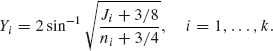
We consider now the normal model
![]()
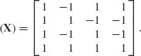
where Y = (Y1, …, Yk)′, η = (η1, …, ηk)′ with ηi = 2sin−1![]() , i = 1, …, k. Moreover, D is a diagonal matrix, D =
, i = 1, …, k. Moreover, D is a diagonal matrix, D = ![]() . Assume a prior multinormal distribution for η.
. Assume a prior multinormal distribution for η.
8.4.9 Consider the normal random walk model, which is a special case of the dynamic linear model (8.4.6), given by
![]()
where θ0 ∼ N(η0, c0), {![]() n} are i.i.d. N(0, σ2) and {ωn} are i.i.d. N(0, τ2). Show that
n} are i.i.d. N(0, σ2) and {ωn} are i.i.d. N(0, τ2). Show that ![]() , where cn is the posterior variance of θn, given (Y1, …, Yn). Find the formula of c*.
, where cn is the posterior variance of θn, given (Y1, …, Yn). Find the formula of c*.
Section 8.5
8.5.1 The integral
![]()
can be computed analytically or numerically. Analytically, it can be computed as

![]()
where ![]() n = X/n. Let k(ω) = log (1 + ω) −
n = X/n. Let k(ω) = log (1 + ω) − ![]() n log(ω) and f(ω) =
n log(ω) and f(ω) = ![]() . Find
. Find ![]() which maximizes -k(ω). Use (8.5.3) and (8.5.4) to approximate I.
which maximizes -k(ω). Use (8.5.3) and (8.5.4) to approximate I.
8.5.2 Prove that if U1, U2 are two i.i.d. rectangular (0, 1) random variables then the Box Muller transformation (8.5.26) yields two i.i.d. N(0, 1) random variables.
8.5.3 Consider the integral I of Problem [1]. How would you approximate I by simulation? How would you run the simulations so that, with probability ≥ 0.95, the absolute error is not greater than 1% of I.
Section 8.6
8.6.1 Let (X1, θ1), …, (Xn, θn), … be a sequence of independent random vectors of which only the Xs are observable. Assume that the conditional distributions of Xi given θi are B(1, θi), i = 1, 2, …, and that θ1, θ2, … are i.i.d. having some prior distribution H(θ) on (0, 1).
8.6.2 Let (X1, ![]() 1), …, (Xn,
1), …, (Xn, ![]() n), … be a sequence of independent random vectors of which only the Xs are observable. It is assumed that the conditional distribution of Xi given
n), … be a sequence of independent random vectors of which only the Xs are observable. It is assumed that the conditional distribution of Xi given ![]() i is NB(
i is NB(![]() i, ν), ν known, i = 1, 2, …. Moreover, it is assumed that
i, ν), ν known, i = 1, 2, …. Moreover, it is assumed that ![]() 1,
1, ![]() 2, … are i.i.d. having a prior distribution H(θ) belonging to the family
2, … are i.i.d. having a prior distribution H(θ) belonging to the family ![]() of beta distributions. Construct a sequence of empirical–Bayes estimators for the squared–error loss, and show that their posterior risks converges a.s. to the posterior risk of the true β (p, q).
of beta distributions. Construct a sequence of empirical–Bayes estimators for the squared–error loss, and show that their posterior risks converges a.s. to the posterior risk of the true β (p, q).
8.6.3 Let (X1, λ1), …, (Xn, λn), … be a sequence of independent random vectors, where Xi | λi ∼ G(λi, 1), i = 1, 2, …, and λ1, λ2, … are i.i.d. having a prior ![]() distribution; τ and ν unknown. Construct a sequence of empirical–Bayes estimators of λi, for the squared–error loss.
distribution; τ and ν unknown. Construct a sequence of empirical–Bayes estimators of λi, for the squared–error loss.
PART IV: SOLUTIONS OF SELECTED PROBLEMS
8.1.6 (i) Since X ∼ N(0, σ2), ![]() . Thus, the density of S, given σ2, is
. Thus, the density of S, given σ2, is
![]()
Let ![]() and let the prior distribution of
and let the prior distribution of ![]() be like that of
be like that of ![]() . Hence, the posterior distribution of
. Hence, the posterior distribution of ![]() , given S, is like that of
, given S, is like that of ![]() .
.
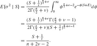
Similarly, we find that
![]()
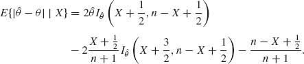
8.1.9
Accordingly,
![]()

8.2.1 (i) The prior risks are R0 = c1π and R1 = c2(1 − π), where π is the prior probability of H0. These two risk lines intersect at π* = c2/(c1 + c2). We have R0(π*) = R1(π*). The posterior probability that H0 is true is
![]()
The Bayes test function is
![]()
![]() π(X) is the probability of rejecting H0. Note that
π(X) is the probability of rejecting H0. Note that ![]() π(X) = 1 if, and only if, X > ξ (π), where
π(X) = 1 if, and only if, X > ξ (π), where
![]()
![]()
Let P(j;λ) denote the c.d.f. of Poisson distribution with mean λ. Then
![]()
and
![]()
![]()
Then
8.3.2 We have a simple linear regression model Yi = α + β xi + ![]() i, i = 1, …, n; where
i, i = 1, …, n; where ![]() i are i.i.d. N(0, σ2). Assume that σ2is known. Let (X) = (1n, xn), where 1n is an n–dimensional vector of 1s, x′n = (x1, …, xn). The model is
i are i.i.d. N(0, σ2). Assume that σ2is known. Let (X) = (1n, xn), where 1n is an n–dimensional vector of 1s, x′n = (x1, …, xn). The model is
![]()
![]()
and
![]()
Accordingly
![]()
Thus, the (1–α) credibility region for θ is
![]()
![]()
8.4.1
![]()
The prior of θ is Beta (p, q), 0 < p, q < ∞.

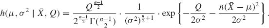
8.4.3 The Jeffreys prior is ![]() . A version of the likelihood function, given the minimal sufficient satistic (
. A version of the likelihood function, given the minimal sufficient satistic (![]() , Q), where Q =
, Q), where Q = ![]() , is
, is
![]()
Thus, the posterior density under Jeffrey’s prior is
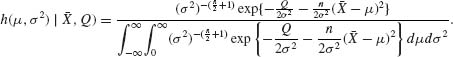
Now,
![]()
Furthermore,
![]()
Accordingly,
Thus, the predictive density of Y, given [![]() , Q], is
, Q], is

or
![]()
Recall that the density of t[n − 1] is
![]()
Thus, the γ–quantile of the predictive distribution fH(y | ![]() , Q) is
, Q) is ![]() +
+ 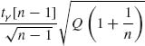 .
.
8.5.3
![]()
where U ∼ β (X + 1, n- X + 1). By simulation, we generate M i.i.d. values of U1, …, UM, and estimate I by ![]()
![]() . For large
. For large ![]() , where D = B2(X +1, n − X + 1)V{e−U}. We have to find M large enough so that
, where D = B2(X +1, n − X + 1)V{e−U}. We have to find M large enough so that ![]() ≥ 0.95. According to the asymptotic normal distribution, we determine M so that
≥ 0.95. According to the asymptotic normal distribution, we determine M so that
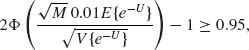
or
![]()
By the delta method, for large M,
![]()
Similarly,
![]()
Hence, M should be the smallest integer such that
