
CHAPTER 2
Statistical Distributions
PART I: THEORY
2.1 INTRODUCTORY REMARKS
This chapter presents a systematic discussion of families of distribution functions, which are widely used in statistical modeling. We discuss univariate and multivariate distributions. A good part of the chapter is devoted to the distributions of sample statistics.
2.2 FAMILIES OF DISCRETE DISTRIBUTIONS
2.2.1 Binomial Distributions
Binomial distributions correspond to random variables that count the number of successes among N independent trials having the same probability of success. Such trials are called Bernoulli trials. The probabilistic model of Bernoulli trials is applicable in many situations, where it is reasonable to assume independence and constant success probability.
Binomial distributions have two parameters N (number of trials) and θ (success probability), where N is a positive integer and 0 < θ < 1. The probability distribution function is denoted by b(i; N, θ) and is
(2.2.1) ![]()
The c.d.f. is designated by B(i; N, θ), and is equal to B(i; N, θ) = 
The Binomial distribution formula can also be expressed in terms of the incomplete beta function by
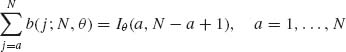
where
(2.2.3) 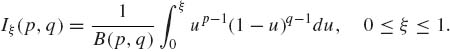
The parameters p and q are positive, i.e., 0 < p, q < ∞; ![]() is the (complete) beta function. Or
is the (complete) beta function. Or
The quantiles B−1(p; N, θ), 0 < p < 1, can be easily determined by finding the smallest value of i at which B(i; N, θ) ≥ p.
2.2.2 Hypergeometric Distributions
The hypergeometric distributions are applicable when we sample at random without replacement from a finite population (collection) of N units, so that every possible sample of size n has equal selection probability, ![]() . If X denotes the number of units in the sample having a certain attribute, and if M is the number of units in the population (before sampling) having the same attribute, then the distribution of X is hypergeometric with the probability density function (p.d.f.)
. If X denotes the number of units in the sample having a certain attribute, and if M is the number of units in the population (before sampling) having the same attribute, then the distribution of X is hypergeometric with the probability density function (p.d.f.)
(2.2.5) 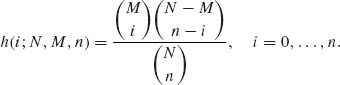
The c.d.f. of the hypergeometric distribution will be denoted by H(i; N, M, n). When n/N is sufficiently small (smaller than 0.1 for most practical applications), we can approximate H(i; N, M, n) by B(i; n, M/N). Better approximations (Johnson and Kotz, 1969, p. 148) are available, as well, as bounds on the error terms.
2.2.3 Poisson Distributions
Poisson distributions are applied when the random variables under consideration count the number of events occurring in a specified time period, or on a spatial area, and the observed processes satisfy the basic conditions of time (or space) homogeneity, independent increments, and no memory of the past (Feller, 1966, p. 566). The Poisson distribution is prevalent in numerous applications of statistics to engineering reliability, traffic flow, queuing and inventory theories, computer design, ecology, etc.
A random variable X is said to have a Poisson distribution with intensity λ, 0 < λ < ∞, if it assumes only the nonnegative integers according to a probability distribution function
(2.2.6) ![]()
The c.d.f. of such a distribution is denoted by P(i; λ).
The Poisson distribution can be obtained from the Binomial distribution by letting N → ∞, θ → 0 so that N θ → λ, where 0 < λ < ∞ (Feller, 1966, p. 153, or Problem 5 of Section 1.10). For this reason, the Poisson distribution can provide a good model in cases of counting events that occur very rarely (the number of cases of a rare disease per 100, 000 in the population; the number of misprints per page in a book, etc.).
The Poisson c.d.f. can be determined from the incomplete gamma function according to the following formula
for all k = 0, 1, …, where
is the gamma function.
2.2.4 Geometric, Pascal, and Negative Binomial Distributions
The geometric distribution is the distribution of the number of Bernoulli trials until the first success. This distribution has therefore many applications (the number of shots at a target until the first hit). The probability distribution function of a geometric random variable is
(2.2.9) ![]()
where θ, 0 < θ < 1, is the probability of success.
If the random variable counts the number of Bernoulli trials until the ν–th success, ν = 1, 2, …, we obtain the Pascal distribution with p.d.f.
(2.2.10) ![]()
The geometric distributions constitute a subfamily with ν = 1. Another family of distributions of this type is that of the Negative–Binomial distributions. We designate by NB(ψ, ν), 0 < ψ < 1, 0 < ν < ∞, a random variable having a Negative–Binomial distribution if its p.d.f. is
(2.2.11) ![]()
Notice that if X has the Pascal distribution with parameters ν and θ, then X – ν is distributed like NB(1 – θ, ν). The probability distribution of Negative–Binomial random variables assigns positive probabilities to all the nonnegative integers. It can therefore be applied as a model in cases of counting random variables where the Poisson assumptions are invalid. Moreover, as we show later, Negative–Binomial distributions may be obtained as averages of Poisson distributions. The family of Negative–Binomial distributions depend on two parameters and can therefore be fitted to a variety of empirical distributions better than the Poisson distributions. Examples of this nature can be found in logistics research in studies of population growth with immigration, etc.
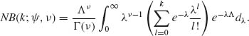
The c.d.f. of the NB(ψ, ν), to be designated as NB(i; ψ, ν), can be determined by the incomplete beta function according to the formula
A proof of this useful relationship is given in Example 2.3.
2.3 SOME FAMILIES OF CONTINUOUS DISTRIBUTIONS
2.3.1 Rectangular Distributions
A random variable X has a rectangular distribution over the interval (θ1, θ2), -∞ < θ1 < θ2 < ∞, if its p.d.f. is
(2.3.1) 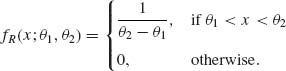
The family of all rectangular distributions is a two–parameter family. We denote r.v.s having these distributions by R(θ1, θ2); -∞ < θ1 < θ2 < ∞. We note that if X is distributed as R(θ1, θ2), then X is equivalent to θ1 + (θ2 – θ1) U, where U ∼ R(0, 1). This can be easily verified by considering the distribution functions of R(θ1, θ2) and of R(0, 1), respectively. Accordingly, the parameter α = θ1 can be considered a location parameter and β = θ2 – θ1 is a scale parameter. Let fU(x) = I{0 ≤ x ≤ 1} be the p.d.f. of the standard rectangular r.v. U. Thus, we can express the p.d.f. of R(θ1, θ2) by the general presentation of p.d.f.s in the location and scale parameter models; namely
The standard rectangular distribution function occupies an important place in the theory of statistics. One of the reasons is that if a random variable has an arbitrary continuous distribution function F(x), then the transformed random variable Y = F(X) is distributed as U. For each ξ, 0 < ξ < 1, let
(2.3.3) ![]()
Accordingly, since F(x) is nondecreasing and continuous,
(2.3.4) ![]()
The transformation X → F(X) is called the Cumulative Probability Integral Transformation.
Notice that the pth quantile of R(θ1, θ2)is
(2.3.5) ![]()
The following has application in the theory of testing hypotheses.
If X has a discrete distribution F(x) and if we define the function
(2.3.6) ![]()
where -∞ < x < ∞ and 0 ≤ γ ≤ 1, then H(X, U) has a rectangular distribution as R(0, 1), where U is also distributed like R(0, 1), independently of X. We notice that if x is a jump point of F(x), then H(x, γ) assumes a value in the interval [F(x – 0), F(x)]. On the other hand, if x is not a jump point, then H(x, γ) = F(x) for all γ. Thus, for every p, 0 ≤ p ≤ 1,
![]()
where
(2.3.7) ![]()
Accordingly, for every p, 0 ≤ p ≤ 1,
(2.3.8) ![]()
2.3.2 Beta Distributions
The family of Beta distributions is a two–parameter family of continuous distributions concentrated over the interval [0, 1]. We denote these distributions by β (p, q); 0 < p, q < ∞. The p.d.f. of a β (p, q) distribution is
(2.3.9) ![]()
The R(0, 1) distribution is a special case. The distribution function (c.d.f.) of β (p, q) coincides over the interval (0, 1) with the incomplete Beta function (2.3.2). Notice that
(2.3.10) ![]()
Hence, the Beta distribution is symmetric about x = .5 if and only if p = q.
2.3.3 Gamma Distributions
The Gamma function Γ (p) was defined in (2.2.8). On the basis of this function we define a two–parameter family of distribution functions. We say that a random variable X has a Gamma distribution with positive parameters λ and p, to be denoted by G(λ, p), if its p.d.f. is
(2.3.11) ![]()
λ−1 is a scale parameter, and p is called a shape parameter. A special important case is that of p = 1. In this case, the density reduces to
(2.3.12) ![]()
This distribution is called the (negative) exponential distribution. Exponentially distributed r.v.s with parameter λ are denoted also as E(λ).
The following relationship between Gamma distributions explains the role of the scale parameter λ−1
(2.3.13) ![]()
Indeed, from the definition of the gamma p.d.f. the following relationship holds for all ξ, 0 ≤ ξ ≤ ∞,
(2.3.14) 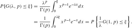
In the case of λ = ![]() and p = ν/2, ν = 1, 2, … the Gamma distribution is also called chi–squared distribution with ν degrees of freedom. The chi–squared random variables are denoted by χ2[ν], i.e.,
and p = ν/2, ν = 1, 2, … the Gamma distribution is also called chi–squared distribution with ν degrees of freedom. The chi–squared random variables are denoted by χ2[ν], i.e.,
(2.3.15) ![]()
The reason for designating a special name for this subfamily of Gamma distributions will be explained later.
2.3.4 Weibull and Extreme Value Distributions
The family of Weibull distributions has been extensively applied to the theory of systems reliability as a model for lifetime distributions (Zacks, 1992). It is also used in the theory of survival distributions with biological applications (Gross and Clark, 1975). We say that a random variable X has a Weibull distribution with parameters (λ, α, ξ); 0 < λ, 0 < α < ∞; -∞ < ξ < ∞, if (X – ξ)α ∼ G(λ, 1). Accordingly, (X – ξ)α has an exponential distribution with a scale parameter λ−1, ξ is a location parameter, i.e., the p.d.f. assumes positive values only for x ≥ ξ. We will assume here, without loss of generality, that ξ = 0. The parameter α is called the shape parameter. The p.d.f. of X, for ξ = 0 is
(2.3.16) ![]()
and its c.d.f. is
(2.3.17) 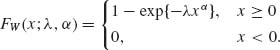
The extreme value distribution (of Type I) is obtained from the Weibull distribution if we consider the distribution of Y = -log X, where Xα ∼ G(λ, 1). Accordingly, the c.d.f. of Y is
(2.3.18) ![]()
-∞ < η < ∞, and its p.d.f. is
- ∞ < x < ∞.
Extreme value distributions have been applied in problems of testing strength of materials, maximal water flow in rivers, biomedical problems, etc. (Gumbel, 1958).
2.3.5 Normal Distributions
The normal distribution occupies a central role in statistical theory. Many of the statistical tests and estimation procedures are based on statistics that have distributions approximately normal in a large sample.
The family of normal distributions, to be designated by N(ξ, σ2), depends on two parameters. A location parameter ξ, -∞ < ξ < ∞ and a scale parameter σ, 0 < σ < ∞. The p.d.f. of a normal distribution is
(2.3.20) 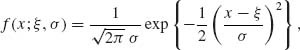
-∞ < x < ∞.
The normal distribution with ξ = 0 and σ = 1 is called the standard normal distribution. The standard normal p.d.f. is denoted by ![]() (x). Notice that N(ξ, σ2) ∼ ξ + σ N(0, 1). Indeed, since σ > 0,
(x). Notice that N(ξ, σ2) ∼ ξ + σ N(0, 1). Indeed, since σ > 0,
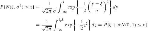
According to (2.3.21), the c.d.f. of N(ξ, σ2) can be computed on the basis of the standard c.d.f. The standard c.d.f. is denoted by Φ(x). It is also called the standard normal integral. Efficient numerical techniques are available for the computation of Φ (x). The function and its derivatives are tabulated. Efficient numerical approximations and asymptotic expansions are given in Abramowitz and Stegun (1968, p. 925). The normal p.d.f. is symmetric about the location parameter ξ. From this symmetry, we deduce that
(2.3.22) ![]()
By a series expansion of e–t2/2 and direct integration, one can immediately derive the formula
(2.3.23) 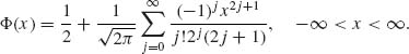
The computation according to this formula is often inefficient. An excellent computing formula was given by Zelen and Severo (1968), namely
(2.3.24) ![]()
where t = (1 + px)-1, p = .2316419; b1 = .3193815; b2 = -.3565638; b3 = 1.7814779; b4 = -1.8212550; b5 = 1.3302744. The magnitude of the error term is |![]() (x)| < 7.5 · 10-8.
(x)| < 7.5 · 10-8.
2.3.6 Normal Approximations
The normal distribution can be used in certain cases to approximate well, the cumulative probabilities of other distribution functions. Such approximations are very useful when it becomes too difficult to compute the exact cumulative probabilities of the distributions under consideration. For example, suppose X ∼ B(100, .35) and we have to compute the probability of the event {X ≤ 88}. This requires the computation of the sum of 89 terms in
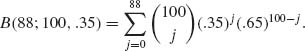
Usually, such a numerical problem requires the use of some numerical approximation and/or the use of a computer. However, the cumulative probability B(88 | 100, .35) can be easily approximated by the normal c.d.f. This approximation is based on the celebrated Central Limit Theorem, which was discussed in Section 1.12. Accordingly, if x ∼ B(n, θ) and n is sufficiently large (relative to θ) then, for 0 ≤ k1 ≤ k2 ≤ n,
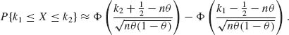
The symbol ![]() designates a large sample approximation.
designates a large sample approximation.
The maximal possible error in using this approximation is less than .14[nθ (1 – θ)]-1/2 (Johnson and Kotz, 1969, p. 64). The approximation turns out to be quite good, even if n is not very large, if θ is close to θ0 = .5. In Table 2.1, we compare the numerically exact c.d.f. values of the Binomial distribution B(k; n, θ) with n = 25 (relatively small) and θ = .25, .40, .50 to the approximation obtained from (2.3.25) with k = k2 and k1 = 0.
Table 2.1 Normal Approximation to the Binomial c.d.f. n = 25
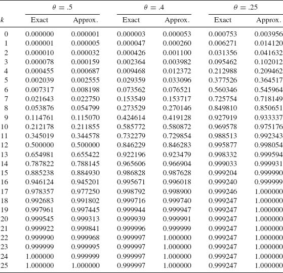
Considerable research has been done to improve the Normal approximation to the Binomial c.d.f. Some of the main results and references are provided in Johnson and Kotz (1969, p. 64).
In a similar manner, the normal approximation can be applied to approximate the Hypergeometric c.d.f. (Johnson and Kotz, 1969, p. 148); the Poisson c.d.f. (Johnson and Kotz, 1969, p. 99) and the Negative–Binomial c.d.f. (Johnson and Kotz, 1969, p. 127).
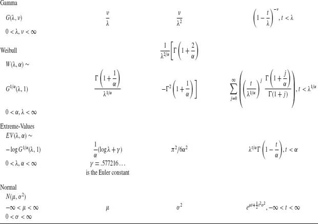
The normal distribution can provide also good approximations to the G(λ, ν) distributions, when ν is sufficiently large, and to other continuous distributions. For a summary of approximating formulae and references see Johnson and Kotz (1969) and Zelen and Severo (1968). In Table 2.2 we summarize important characteristics of the above distribution functions.
Table 2.2 Expectations, Variances and Moment Generating Functions of Selected Distributions

2.4 TRANSFORMATIONS
2.4.1 One–to–One Transformations of Several Variables
Let X1, …, Xk be random variables of the continuous type with a joint p.d.f. f(x1, …, xk). Let yi = gi(xi, …, xk), i = 1, …, k, be one–to–one transformations, and let xi = ψi(y1, …, yk) i = 1, …, k, be the inverse transformations. Assume that ![]() are continuous for all i, j = 1, …, k at all points (y1, …, yk). The Jacobian of the transformation is
are continuous for all i, j = 1, …, k at all points (y1, …, yk). The Jacobian of the transformation is
(2.4.1) ![]()
where det.(·) denotes the determinant of the matrix of partial derivatives. Then the joint p.d.f. of (Y1, …, Yk) is
(2.4.2) ![]()
2.4.2 Distribution of Sums
Let X1, X2 be absolutely continuous random variables with a joint p.d.f. f(x1, x2). Consider the one–to–one transformation Y1 = X1, Y2 = X1 + X2. It is easy to verify that J(y1, y2) = 1. Hence,
![]()
Integrating over the range of Y1 we obtain the marginal p.d.f. of Y2, which is the required p.d.f. of the sum. Thus, if g(y) denotes the p.d.f. of Y2
(2.4.3) ![]()
If X1 and X2 are independent, having marginal p.d.f.s f1(x) and f2(x), the p.d.f. of the sum g(y) is the convolution of f1(x) and f2(x), i.e.,
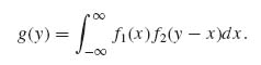
If X1 is discrete, the integral in (2.4.4) is replaced by a sum over the jump points of F1 (x). If there are more than two variables, the distribution of the sum can be found by a similar method.
2.4.3 Distribution of Ratios
Let X1, X2 be absolutely continuous with a joint p.d.f., f(x1, x2). We wish to derive the p.d.f. of R = X1/X2. In the general case, X2 can be positive or negative and therefore we separate between the two cases. Over the set -∞ < x1 < ∞, 0 < x2 < ∞ the transformation R = X1 /X2 and Y = X2 is one–to–one. It is also the case over the set -∞ < x1 < ∞, -∞ < x2 < 0. The Jacobian of the inverse transformation is J(y, r) = –y. Hence, the p.d.f. of R is
(2.4.5) ![]()
The result of Example 2.2 has important applications.
Let X1, X2, …, Xk be independent random variables having gamma distributions with equal λ, i.e., Xi ∼ G(λ, νi), i = 1, …, k. Let T = ![]() and for i = 1, …, k – 1
and for i = 1, …, k – 1
![]()
The marginal distribution of Yi is β 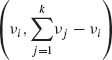 . The joint distribution of Y = (Y1, …, Yk-1) is called the Dirichlet distribution,
 ![]() (ν1, ν2, …, νk), whose joint p.d.f. is
(ν1, ν2, …, νk), whose joint p.d.f. is
(2.4.6) 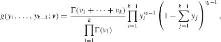
for  .
.
The p.d.f. of ![]() (ν1, …, νk) is a multivariate generalization of the beta distribution.
(ν1, …, νk) is a multivariate generalization of the beta distribution.
Let  . One can immediately prove that for all i, i′ = 1, …, k – 1
(2.4.7) ![]()
and thus
Additional properties of the Dirichlet distributions are specified in the exercises.
2.5 VARIANCES AND COVARIANCES OF SAMPLE MOMENTS
A random sample is a set of n (n ≥ 1) independent and identically distributed (i.i.d.) random variables, having a common distribution F(x). We assume that F has all moments required in the following development. The rth moment of F, r ≥ 1, is μr.
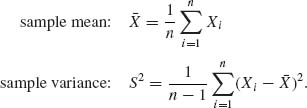
The rth sample moment is
(2.5.1) ![]()
We immediately obtain that
(2.5.2) 
since all Xi are identically distributed. Notice that due to independence, cov(Xi, Xj) = 0 for all i ≠ j. We present here a method for computing ![]() and
and ![]() for r ≠ r′. We consider expansions of the form
for r ≠ r′. We consider expansions of the form  , in terms of augmented symmetric functions and introduce the following notation
(2.5.3) ![]()
(2.5.4) ![]()
(2.5.5) ![]()
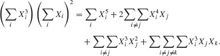
etc. The sum of powers in such an expression is called the weight of [ ]. Thus, the weight of [l1l2l3] is w = l1 + l2 + l3. In Table 2.3, we find expansions of (l1)α1 (l2)α2… in terms of multi–sums ![]() . For additional values of coefficients for such expansions, see David and Kendall (1955). For example, to expand
. For additional values of coefficients for such expansions, see David and Kendall (1955). For example, to expand  the weight is w = 5, and according to Table 2.3, (3)(1)2 = [5] + 2[41] + [32] + [312].
Table 2.3 Augmented Symmetric Functions in Terms of Power–Series
| Weight | ( ) | [ ] |
| 2 | (2) | [2] |
| (1)2 | [2] + [12] | |
| 3 | (3) | [3] |
| (2)(1) | [3] + [21] | |
| (1)3 | [3] + 3[21] + [13] | |
| 4 | (4) | [4] |
| (3)(1) | [4] + [31] | |
| (2)2 | [4] + [22] | |
| (2)(1)2 | [4] + 2[31] + [22] + [212] | |
| (1)4 | [4] + 4[31] + 3[22] + 6[212] + [14] | |
| 5 | (5) | [5] |
| (4)(1) | [5] + [41] | |
| (3)(2) | [5] + [32] | |
| (3)(1)2 | [5] + 2[41] + [32] + [312] | |
| (2)2(1) | [5] + [41] + 2[32] + [221] | |
| (2)(1)3 | [5] + 3[41] + 4[32] + 3[312] + 3[221] + [213] | |
| (1)5 | [5] + 5[41] + 10[32] + 10[312] + 15[221] + 10[213] + [15] | |
| 6 | (6) | [6] |
| (5)(1) | [6] + [51] | |
| (4)(2) | [6] + [42] | |
| (4)(12) | [6] + 2[51] + [42] + [412] | |
| (3)2 | [6] + [32] | |
| (3)(2)(1) | [6] + [51] + [42] + [32] + [321] | |
| (3)(1)3 | [6] + 3[51] + 3[42] + 3[412] + [32] + 3[321] + [313] | |
| (2)3 | [6] + 3[42] + [23] | |
| (2)2(1)2 | [6] + 2[51] + 3[42] + [412] + 2[32] + 4[321] + [23] + [2212] | |
| (2)(1)4 | [6] + 4[51] + 7[42] + 6[412] + 4[32] + 16[32] | |
| +, 4[313] + 3[23] + 6[2212] + [214] | ||
| (1)6 | [6] + 6[51] + 15[42] + 15[412] + 10[32] + 60[321] | |
| +, 20[313] + 15[23] + 45[2212] + 15[214] + [16] |
(*) [32]=[33], etc.
Source: Compiled from David and Kendall (1955).
Thus,
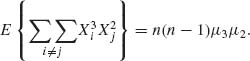
The expected values of such expansions are given in terms of product of the moments (independence) times the number of terms in the sum, e.g.,
2.6 DISCRETE MULTIVARIATE DISTRIBUTIONS
2.6.1 The Multinomial Distribution
Consider an experiment in which the result of each trial belongs to one of k alternative categories. Let θ′ = (θ1, …, θk) be a probability vector, i.e., 0 < θi < 1 for all i = 1, …, k and ![]() = 1. θi designates the probability that the outcome of an individual trial belongs to the ith category. Consider n such independent trials, n ≥ 1, and let X = (X1, …, Xk) be a random vector. Xi is the number of trials in which the ith category is realized,
= 1. θi designates the probability that the outcome of an individual trial belongs to the ith category. Consider n such independent trials, n ≥ 1, and let X = (X1, …, Xk) be a random vector. Xi is the number of trials in which the ith category is realized, ![]() = n. The distribution of X is given by the multinomial probability distribution
= n. The distribution of X is given by the multinomial probability distribution
(2.6.1) 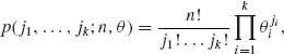
where ji = 0, 1, …, n and ![]() = n. These terms are obtained by the multinomial expansion of (θ1 + … + θk)n. Hence, their sum equals 1. We will designate the multinomial distribution based on n trials and probability vector θ by M(n, θ). The binomial distribution is a special case, when k = 2. Moreover, the marginal distribution of Xi is the binomial B(n, θi). The joint marginal distribution of any pair (Xi, Xi′) where 1 ≤ i < i′ ≤ k is the corresponding trinomial, with probability distribution function
= n. These terms are obtained by the multinomial expansion of (θ1 + … + θk)n. Hence, their sum equals 1. We will designate the multinomial distribution based on n trials and probability vector θ by M(n, θ). The binomial distribution is a special case, when k = 2. Moreover, the marginal distribution of Xi is the binomial B(n, θi). The joint marginal distribution of any pair (Xi, Xi′) where 1 ≤ i < i′ ≤ k is the corresponding trinomial, with probability distribution function
(2.6.2) 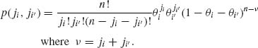
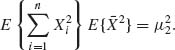
We consider now the moments of the multinomial distribution. From the marginal Binomial distribution of the Xs we have
(2.6.3) ![]()
To obtain the covariance of Xi, Xj, i ≠ j we proceed in the following manner. If n = 1 then E{Xi Xj} = 0 for all i ≠ j, since only one of the components of X is one and all the others are zero. Hence, E{Xi Xj} – E{Xi} E{Xj} = –θi θj if i ≠ j. If n > 1, we obtain the result by considering the sum of n independent vectors. Thus,
We conclude the section with a remark about the joint moment generating function (m.g.f.) of the multinomial random vector X. This function is defined in the following manner. Since Xk =  , we define for every k ≥ 2
(2.6.5) 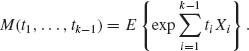
One can prove by induction on k that
(2.6.6) 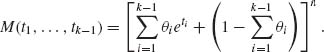
2.6.2 Multivariate Negative Binomial
Let X = (X1, …, Xk) be a k–dimensional random vector. Each random variable, Xi, i = 1, …, k, can assume only nonnegative integers. Their joint probability distribution function is given by
(2.6.7) 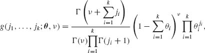
where j1, …, jk = 0, 1, …; 0 < ν < ∞, 0 < θi < 1 for each i = 1, …, k and  . We develop here the basic theory for the case of k = 2. (For k = 1 the distribution reduces to the univariate NB(θ, ν). Summing first with respect to j2 we obtain
(2.6.8) 
Hence, the marginal of Xi is
(2.6.9) ![]()
where nb(j; ψ, ν) is the p.d.f. of the negative binomial NB(ψ, ν). By dividing the joint probability distribution function g(j1, j2;θ1, θ2, ν) by ![]() , we obtain that the conditional distribution of X2 given X1 is the negative binomial NB(θ2, ν + X1). Accordingly, if NB(θ1, θ2, ν) designates a bivariate negative binomial with parameters (θ1, θ2, ν), then the expected value of Xi is given by
, we obtain that the conditional distribution of X2 given X1 is the negative binomial NB(θ2, ν + X1). Accordingly, if NB(θ1, θ2, ν) designates a bivariate negative binomial with parameters (θ1, θ2, ν), then the expected value of Xi is given by
(2.6.10) ![]()
The variance of the marginal distribution is
(2.6.11) ![]()
Finally, to obtain the covariance between X1 and X2 we determine first
(2.6.12) 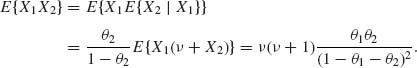
Therefore,
(2.6.13) ![]()
We notice that, contrary to the multinomial case, the covariances of any two components of the multivariate negative binomial vector are all positive.
2.6.3 Multivariate Hypergeometric Distributions
This family of k–variate distributions is derived by a straightforward generalization of the univariate model. Accordingly, suppose that a finite population of elements contain M1 of type 1, M2 of type 2, …, Mk of type k and  of other types. A sample of n elements is drawn at random and without replacement from this population. Let Xi, i = 1, …, k denote the number of elements of type i observed in the sample. The p.d.f. of X = (X1, …, Xk) is
(2.6.14) 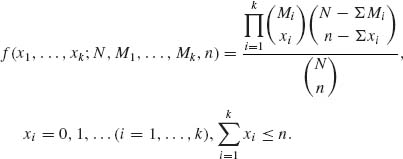
One immediately obtains that the marginal distributions of the components of X are hypergeometric distributions, with parameters (N, Mi, n), i = 1, …, k. If we designate by H(N, M1, …, Mk, n) the multivariate hypergeometric distribution, then the conditional distribution of (Xr + 1, …, Xk) given (X1 = j1, …, Xr = jr) is the hypergeometric 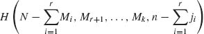 . Using this result and the law of the iterated expectation we obtain the following result, for all i ≠ j,
(2.6.15) ![]()
This result is similar to that of the multinomial (2.6.4), which corresponds to sampling with replacement.
2.7 MULTINORMAL DISTRIBUTIONS
2.7.1 Basic Theory
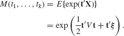
A random vector (X1, …, Xk) of the continuous type has a k–variate multinormal distribution if its joint p.d.f. can be expressed in vector and matrix notation as
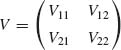
for -∞ < ξi < ∞, i = 1, …, k. Here, x = (x1, …, xk)′, ξ} = (ξ1, …, ξk)′. V is a k × k symmetric positive definite matrix and |V| is the determinant of V. We introduce the notation X ∼ N(ξ}, V). We notice that the k–variate multinormal p.d.f. (2.7.1) is symmetric about the point ξ. Hence, ξ is the expected value (mean) vector of X. Moreover, all the moments of X exist.
The m.g.f. of X is
To establish formula (2.7.2) we can assume, without loss of generality, that ξ = 0, since if MX(t) is the m.g.f. of X and Y = X + b, then the m.g.f. of Y is MY(t) = exp(t′b)MX(t). Thus, we have to determine
(2.7.3) 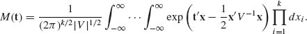
Since V is positive definite, there exists a nonsingular matrix D such that V = DD′. Consider the transformation Y = D−1X; then x′V−1x = y′y and t′x = t′Dy. Therefore,
(2.7.4) ![]()
Finally, the Jacobian of the transformation is |D| and
(2.7.5) 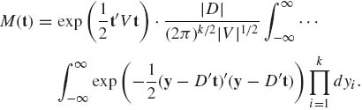
Since |D| = |V|1/2 and (2π)–k/2 times the multiple integral on the right–hand side is equal to one, we establish (2.7.2). In order to determine the variance–covariance matrix of X we can assume, without loss of generality, that its expected value is zero. Accordingly, for all i, j,
From (2.7.2) and (2.7.6), we obtain that cov(Xi, Xj) = σij. (i, j = 1, …, k), where σij is the (i, j)th element of V. Thus, V is the variance–covariance matrix of X.
A k–variate multinormal distribution is called standard if ξi = 0 and σii = 1 for all i = 1, …, k. In this case, the variance matrix will be denoted by R since its elements are the correlations between the components of X. A standard normal vector is often denoted by Z, its joint p.d.f. and c.d.f. by ![]() k(z | R) and Φk(z | R), respectively.
k(z | R) and Φk(z | R), respectively.
2.7.2 Distribution of Subvectors and Distributions of Linear Forms
In this section we present several basic results without proofs. The proofs are straightforward and the reader is referred to Anderson (1958) and Graybill (1961).
Suppose that a k–dimensional vector X has a multinormal distribution N(μ, V). We consider the two subvectors Y and Z, i.e., X′ = (Y′, Z′), where Y is r–dimensional, 1 ≤ r < k.
Partition correspondingly the expectation vector ξ to ξ′ = (η′, ζ′) and the covariance matrix to
The following results are fundamental to the multinormal theory.
and an analogous formula can be obtained for the conditional distribution of Z given Y.
The conditional expectation
is called the linear regression of Y on Z. The conditional covariance matrix
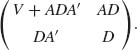
represents the variances and covariances of the components of Y around the linear regression hyperplane. The above results have the following converse counterpart. Suppose that Y and Z are two vectors such that
and
then the marginal distribution of Y is the multinormal
![]()
and the joint distribution of Y and Z is the multinormal, with expectation vector (ζ′ A′, ζ′)′ and a covariance matrix
Finally, if X∼ N(ξ, V) and Y = b + AX, then Y ∼ N(b + Aξ, AVA′). That is, every linear combination of normally distributed random variables is normally distributed.
In the case of k = 2, the multinormal distribution is called a bivariate normal distribution. The joint p.d.f. of a bivariate normal distribution is
(2.7.9) 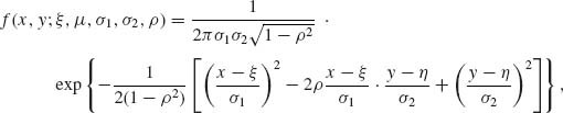
-∞ < x, y < ∞.
The parameters ξ and η are the expectations, and ![]() and
and ![]() are the variances of X and Y, respectively. ρ is the coefficient of correlation.
are the variances of X and Y, respectively. ρ is the coefficient of correlation.
The conditional distribution of Y given {X = x} is normal with conditional expectation
(2.7.10) ![]()
where β = ρ σ2/σ1. The conditional variance is
(2.7.11) ![]()
These formulae are special cases of (2.7.7) and (2.7.8). Since the joint p.d.f. of (X, Y) can be written as the product of the conditional p.d.f. of Y given X, with the marginal p.d.f. of X, we obtain the expression,
(2.7.12) 
This expression can serve also as a basis for an algorithm to compute the Bivariate–Normal c.d.f., i.e.,
(2.7.13) 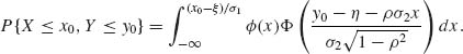
Let Z1, Z2 and Z3 have a joint standard Trivariate–Normal distribution, with a correlation matrix
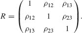
The conditional Bivariate–Normal distribution of (Z1, Z2) given Z3 has a covariance matrix
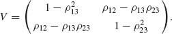
The conditional correlation between Z1 and Z2, given Z3 can be determined from (2.7.14). It is called the partial correlation of Z1, Z2 under Z3 and is given by
2.7.3 Independence of Linear Forms
Let X = (X1, …, Xk)′ be a multinormal random vector. Without loss of generality, assume that E{X} = 0. Let V be the covariance matrix of X. We investigate first the conditions under which two linear functions Y1 = α′X and Y2 = β′X are independent.
Let Y = (Y1, Y2)′, A = ![]() . That is, A is a 2 × k matrix and Y = AX. Y has a bivariate normal distribution with a covariance matrix AVA′. Y1 and Y2 are independent if and only if cov(Y1, Y2) = 0. Moreover, cov(Y1, Y2) = α′Vβ. Since V is positive definite there exists a nonsingular matrix C such that V = CC′. Accordingly, cov(Y1, Y2) = 0 if and only if (C′α)′ (C′β) = 0. This means that the vectors C′α and C′β should be orthogonal. This condition is generalized in a similar fashion to cases where Y1 and Y2 are vectors. Accordingly, if Y1 = AX and Y2 = BX, then Y1 and Y2 are independent if and only if AVB′ = 0. In other words, the column vectors of CA′ should be mutually orthogonal to the column vectors of C′B.
. That is, A is a 2 × k matrix and Y = AX. Y has a bivariate normal distribution with a covariance matrix AVA′. Y1 and Y2 are independent if and only if cov(Y1, Y2) = 0. Moreover, cov(Y1, Y2) = α′Vβ. Since V is positive definite there exists a nonsingular matrix C such that V = CC′. Accordingly, cov(Y1, Y2) = 0 if and only if (C′α)′ (C′β) = 0. This means that the vectors C′α and C′β should be orthogonal. This condition is generalized in a similar fashion to cases where Y1 and Y2 are vectors. Accordingly, if Y1 = AX and Y2 = BX, then Y1 and Y2 are independent if and only if AVB′ = 0. In other words, the column vectors of CA′ should be mutually orthogonal to the column vectors of C′B.
2.8 DISTRIBUTIONS OF SYMMETRIC QUADRATIC FORMS OF NORMAL VARIABLES
In this section, we study the distributions of symmetric quadratic forms in normal random variables. We start from the simplest case.
Case A:
![]()
Assume first that σ2 = 1. The density of X is then ![]() (x) =
(x) = ![]() exp
exp![]() . Therefore, the p.d.f. of Q is
. Therefore, the p.d.f. of Q is
(2.8.1) 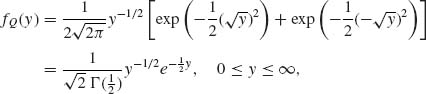
since ![]() .
.
Comparing fQ(y) with the p.d.f. of the gamma distributions, we conclude that if σ2 = 1 then Q ∼ G![]() ∼ χ2 [1]. In the more general case of arbitrary σ2, Q ∼ σ2χ2[1].
∼ χ2 [1]. In the more general case of arbitrary σ2, Q ∼ σ2χ2[1].
Case B:
![]()
This is a more complicated situation. We shall prove that the p.d.f. of Q (and so its c.d.f. and m.g.f.) is, at each point, the expected value of the p.d.f. (or c.d.f. or m.g.f.) of σ2χ2[1 + 2J], where J is a Poisson random variable with mean
Such an expectation of distributions is called a mixture. The distribution of Q when σ2 = 1 is called a noncentral chi–squared with 1 degree of freedom and parameter of noncentrality λ. In symbols Q ∼ χ2[1;λ]. When λ = 0, the noncentral chi–squared coincides with the chi–squared, which is also called central chi–squared. The proof is obtained by determining first the m.g.f. of Q. As before, assume that σ2 = 1. Then,
(2.8.3) ![]()
Write, for all t < ![]() ,
,
(2.8.4) ![]()
Thus,
(2.8.5) ![]()
Furthermore, ![]() . Hence,
. Hence,
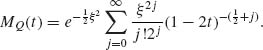
According to Table 2.2, ![]() is the m.g.f. of χ2[1+2j]. Thus, according to (2.8.6) the m.g.f. of χ2[1;λ] is the mixture of the m.g.f.s of χ2[1+2J], where J has a Poisson distribution, with mean λ as in (2.8.2). This implies that the distribution of χ2[1;λ] is the marginal distribution of X in a model where (X, J) have a joint distribution, such that the conditional distribution of X given {J = j} is like that of χ2[1+2j] and the marginal distribution of J is Poisson with expectation λ. From Table 2.2, we obtain that E{χ2[ν]} = ν and V{χ2[ν]} = 2ν. Hence, by the laws of the iterated expectation and total variance
is the m.g.f. of χ2[1+2j]. Thus, according to (2.8.6) the m.g.f. of χ2[1;λ] is the mixture of the m.g.f.s of χ2[1+2J], where J has a Poisson distribution, with mean λ as in (2.8.2). This implies that the distribution of χ2[1;λ] is the marginal distribution of X in a model where (X, J) have a joint distribution, such that the conditional distribution of X given {J = j} is like that of χ2[1+2j] and the marginal distribution of J is Poisson with expectation λ. From Table 2.2, we obtain that E{χ2[ν]} = ν and V{χ2[ν]} = 2ν. Hence, by the laws of the iterated expectation and total variance
(2.8.7) ![]()
and
(2.8.8) ![]()
Case C:
X1, …, Xn are independent; Xi ∼ N(ξi, σ2), i = 1, …, n,
![]()
It is required that all the variances σ2 are the same. As proven in Case B,
(2.8.9) ![]()
where Ji ∼ P(λi).
Consider first the conditional distribution of Q given (J1, …, Jn). From the result on the sum of independent chi–squared random variables, we infer
(2.8.10) 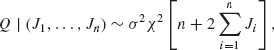
where Q | (J1, …, Jn) denotes the conditional equivalence of the random variables. Furthermore, since the original Xi s are independent, so are the Ji s and therefore
(2.8.11) ![]()
Hence, the marginal distribution of Q is the mixture of σ2χ2[n + 2M] where M ∼ P(λ1 + … + λn). We have thus proven that
(2.8.12) ![]()
Case D:
![]()
where A is a real symmetric matrix. The following is an important result.
(2.8.13) ![]()
if and only if VA is an idempotent matrix of rank r (Graybill, 1961). The proof is based on the fact that every positive definite matrix V can be expressed as V = CC′, where C is nonsingular. If Y = C−1X then Y ∼ N(C−1ξ, I) and X′AX = Y′C′ACY. C′AC is idempotent if and only if VA is idempotent.
The following are important facts about real symmetric idempotent matrices.
2.9 INDEPENDENCE OF LINEAR AND QUADRATIC FORMS OF NORMAL VARIABLES
Without loss of generality, we assume that X ∼ N(0, I). Indeed, if X ∼ N(0, V) and V = CC′ make the transformation X* = C−1X, then X* ∼ N(0, I). Let Y = BX and Q = X′ AX, where A is idempotent of rank r, 1 ≤ r ≤ k. B is an n × k matrix of full rank, 1 ≤ n ≤ k.
Theorem 2.9.1 Y and Q are independent if and only if
(2.9.1) ![]()
For proof, see Graybill (1961, Ch. 4).
Suppose now that we have m quadratic forms X′Bi X in a multinormal vector X ∼ N(ξ}, I).
Theorem 2.9.2 If X ∼ Nξ, I) the set of positive semidefinite quadratic forms X′Bi X (i = 1, …, m) are jointly independent and X′Bi X∼ χ2[ri;λi], where ri is the rank of Bi and λi =![]() , if any two of the following three conditions are satisfied.
, if any two of the following three conditions are satisfied.
This theorem has many applications in the theory of regression analysis, as will be shown later.
2.10 THE ORDER STATISTICS
Let X1, …, Xn be a set of random variables (having a joint distribution). The order statistic is
(2.10.1) ![]()
where X(1) ≤ X(2) ≤ … ≤ X(n).
If X1, …, Xn are independent random variables having an identical absolutely continuous distribution function F(x) with p.d.f. f(x), then the p.d.f. of the order statistic is
To obtain the p.d.f. of the ith order statistic X(i), i = 1, …, n, we can integrate (2.10.2) over the set
(2.10.3) ![]()
This integration yields the p.d.f.
-∞ < ξ < ∞. We can obtain this result also by a nice probabilistic argument. Indeed, for all dx sufficiently small, the trinomial model yields
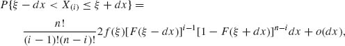
where o(dx) is a function of dx that approaches zero at a faster rate than dx, i.e., o(dx)/dx → 0 as dx → 0.
Dividing (2.10.5) by 2dx and taking the limit as dx → 0, we obtain (2.10.4). The joint p.d.f. of (X(i), X(j)) with 1≤ i < j ≤ n is obtained similarly as
(2.10.6) 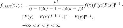
In a similar fashion we can write the joint p.d.f. of any set of order statistics. From the joint p.d.f.s of order statistics we can derive the distribution of various functions of the order statistics. In particular, consider the sample median and the sample range.
The sample median is defined as
(2.10.7) 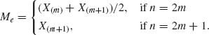
That is, half of the sample values are smaller than the median and half of them are greater. The sample range Rn is defined as
(2.10.8) ![]()
In the case of absolutely continuous independent r.v.s, having a common density f(x), the density g(x) of the sample median is
(2.10.9) 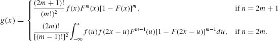
We derive now the distribution of the sample range Rn. Starting with the joint p.d.f. of (X(1), X(n))
(2.10.10) ![]()
we make the transformation u = x, r = y – x.
The Jacobian of this transformation is J = 1 and the joint density of (u, r) is
(2.10.11) ![]()
Accordingly, the density of Rn is
(2.10.12) ![]()
For a comprehensive development of the theory of order statistics and interesting applications, see the books of David (1970) and Gumbel (1958).
2.11 t–DISTRIBUTIONS
In many problems of statistical inference, one considers the distribution of the ratio of a statistic, which is normally distributed to its standard–error (the square root of its variance). Such ratios have distributions called the t–distributions. More specifically, let U ∼ N(0, 1) and W ∼ (χ2[ν]/ν)1/2, where U and W are independent. The distribution of U/W is called the “student’s t–distribution.” We denote this statistic by t[ν] and say that U/W is distributed as a (central) t[ν] with ν degrees of freedom.
An example for the application of this distribution is the following. Let X1, …, Xn be i.i.d. from a N(ξ, σ2) distribution. We have proven that the sample mean ![]() is distributed as
is distributed as ![]() and is independent of the sample variance S2, where S2 ∼ σ2χ2[n – 1]/(n – 1). Hence,
and is independent of the sample variance S2, where S2 ∼ σ2χ2[n – 1]/(n – 1). Hence,
(2.11.1) ![]()
To find the moments of t[ν] we observe that, since the numerator and denominator are independent,
(2.11.2) ![]()
Thus, all the existing odd moments of t[ν] are equal to zero, since E{Ur} = 0 for all r = 2m + 1. The existence of E{(t[ν])r} depends on the existence of E(χ2[ν]/ν)−r/2}. We have
(2.11.3) ![]()
Accordingly, a necessary and sufficient condition for the existence of E{(t[ν])r} is ν > r. Thus, if ν > 2 we obtain that
(2.11.4) ![]()
This is also the variance of t[ν]. We notice that V{t[ν]} → 1 as ν → ∞. It is not difficult to derive the p.d.f. of t[ν], which is
(2.11.5) ![]()
The c.d.f. of t[ν] can be expressed in terms of the incomplete beta function. Due to the symmetry of the distribution around the origin
(2.11.6) ![]()
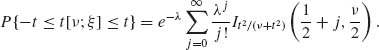
We consider now the distribution of (U + ξ)/W, where ξ is any real number. This ratio is called the noncentral t with ν degrees of freedom, and parameter of noncentrality ξ. This variable is the ratio of two independent random variables namely N(ξ, 1) to (χ2[ν]/ν)1/2. If we denote the noncentral t by t[ν ;ξ], then
Since the random variables in the numerator and denominator of (2.11.7) are independent, one obtains
and that the central moments of orders 2 and 3 are
(2.11.9) 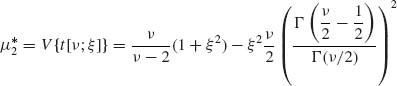
and
(2.11.10) 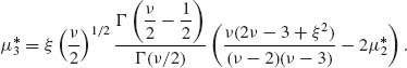
This shows that the t[ν ;ξ] is not symmetric. Furthermore, since U + ξ ∼ – U + ξ we obtain that, for all –∞ < ξ < ∞,
(2.11.11) ![]()
In particular, we have seen this in the central case (ξ = 0). The formulae of the p.d.f. and the c.d.f. of the noncentral t[ν ;ξ] are quite complicated. There exists a variety of formulae for numerical computations. We shall not present these formulae here; the interested reader is referred to Johnson and Kotz (1969, Ch. 31). In the following section, we provide a representation of these distributions in terms of mixtures of beta distributions.
The univariate t–distribution can be generalized to a multivariate–t in a variety of ways. Consider an m–dimensional random vector X having a multinomial distribution N(ξ, σ2 R), where R is a correlation matrix. This is the case when all components of X have the same variance σ2. Recall that the marginal distribution of
![]()
Thus, if S2 ∼ σ2 χ2[ν]/ν independently of Y1, …, Ym, then
![]()
have the marginal t–distributions t[ν]. The p.d.f. of the multivariate distribution of ![]() is given by
is given by
(2.11.12) 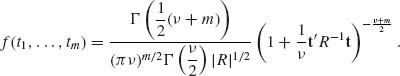
Generally, we say that X has a t[ν ; ξ, ![]() ] distribution if its multivariate p.d.f. is
] distribution if its multivariate p.d.f. is
(2.11.13) ![]()
This distribution has applications in Bayesian analysis, as shown in Chapter 8.
2.12 F–DISTRIBUTIONS
The F–distributions are obtained by considering the distributions of ratios of two independent variance estimators based on normally distributed random variables. As such, these distributions have various important applications, especially in the analysis of variance and regression (Section 4.6). We introduce now the F–distributions formally. Let χ2[ν1] and χ2[ν2] be two independent chi–squared random variables with ν1 and ν2 degrees of freedom, respectively. The ratio
(2.12.1) ![]()
is called an F–random variable with ν1 and ν2 degrees of freedom. It is a straightforward matter to derive the p.d.f. of F[ν1, ν2], which is given by
(2.12.2) 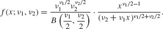
The cumulative distribution function can be computed by means of the incomplete beta function ratio according to the following formula
where
In order to derive this formula, we recall that if ![]() and
and ![]() are two independent gamma random variables, then (see Example 2.2)
are two independent gamma random variables, then (see Example 2.2)
Hence,
(2.12.6) 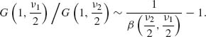
We thus obtain
(2.12.7) 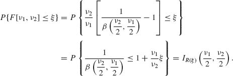
For testing statistical hypotheses, especially for the analysis of variance and regression, one needs quantiles of the F[ν1, ν2] distribution. These quantiles are denoted by Fp [ν1, ν2] and are tabulated in various statistical tables. It is easy to establish the following relationship between the quantiles of F[ν1, ν2] and those of F[ν2, ν1], namely,
(2.12.8) ![]()
The quantiles of the F[ν1, ν2] distribution can also be determined by those of the beta distribution by employing formula (2.12.5). If we denote by βγ (p, q) the values of x for which Ix (p, q) = γ, we obtain from (2.12.4) that
(2.12.9) ![]()
The moments of F[ν1, ν2] are obtained in the following manner. For a positive integer r
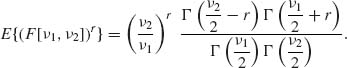
We realize that the rth moment of F[ν1, ν2] exists if and only if ν2 > 2r. In particular,
(2.12.11) ![]()
Similarly, if ν2 > 4 then
(2.12.12) ![]()
In various occasions one may be interested in an F–like statistic, in which the ratio consists of a noncentral chi–squared in the numerator. In this case the statistic is called a noncentral F. More specifically, let χ2[ν1;λ] be a noncentral chi–squared with ν1 degrees of freedom and a parameter of noncentrality λ. Let χ2[ν2] be a central chi–squared with ν2 degrees of freedom, independent of the noncentral chi–squared. Then
(2.12.13) ![]()
is called a noncentral F[ν1, ν2;λ] statistic. We have proven earlier that χ2[ν1;λ] ∼ χ2[ν1 + 2J], where J has a Poisson distribution with expected value λ. For this reason, we can represent the noncentral F[ν1, ν2;λ] as a mixture of central F statistics.
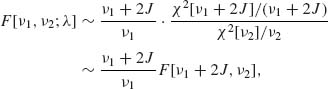
where J ∼ P (λ). Various results concerning the c.d.f. of F[ν1, ν2;λ], its moments, etc., can be obtained from relationship (2.12.14). The c.d.f. of the noncentral F statistic is
Furthermore, following (2.12.3) we obtain
![]()
where
![]()
As in the central case, the moments of the noncentral F are obtained by employing the law of the iterated expectation and (2.12.14). Thus,
However, for all j = 0, 1, …, E{F[ν1 + 2j, ν2]} = ν2/(ν2-2). Hence,
(2.12.17) 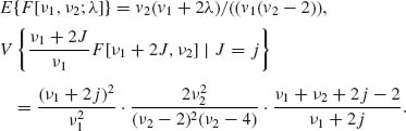
Hence, applying the law of the total variance
(2.12.18) ![]()
We conclude the section with the following observation on the relationship between t– and the F–distributions. According to the definition of t[ν] we immediately obtain that
(2.12.19) ![]()
Hence,
(2.12.20) ![]()
Moreover, due to the symmetry of the t[ν] distribution, for t > 0 we have 2P{t[ν] ≤ t} = 1 + P{F[1, ν] ≤ t2}, or
(2.12.21) ![]()
In a similar manner we obtain a representation for P{|t[ν, ξ]| ≤ t}. Indeed, (N(0, 1) + ξ)2 ∼ χ2 [1;λ] where λ = ![]() . Thus, according to (2.12.16)
. Thus, according to (2.12.16)
2.13 THE DISTRIBUTION OF THE SAMPLE CORRELATION
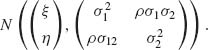
Consider a sample of n i.i.d. vectors (X1, Y1), …, (Xn, Yn) that have a common bivariate normal distribution
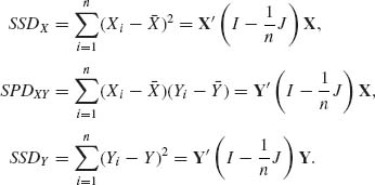
In this section we develop the distributions of the following sample statistics.
(2.13.1) ![]()
(2.13.2) ![]()
where
As mentioned earlier, the joint density of (X, Y) can be written as
(2.13.4) 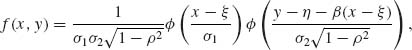
where β = ρ σ2/σ1. Hence, if we make the transformation
(2.13.5) ![]()
then Ui and Vi are independent random variables, ![]() and
and ![]() . We consider now the distributions of the variables
. We consider now the distributions of the variables
(2.13.6) 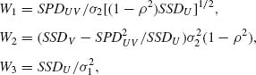
where SSDU, SPDUV and SSDV are defined as in (2.13.3) in terms of (Ui, Vi), i = 1, …, n. Let U = (U1, …, Un)′ and V = (V1, …, Vn)′. We notice that the conditional distribution of SPDUV = ![]() given U is the normal
given U is the normal ![]() . Hence, the conditional distribution of W1 given U is N(0, 1). This implies that W1 is N(0, 1), independently of U. Furthermore, W1 and W3 are independent, and W3 ∼ χ2[n – 1]. We consider now the variable W2. It is easy to check
. Hence, the conditional distribution of W1 given U is N(0, 1). This implies that W1 is N(0, 1), independently of U. Furthermore, W1 and W3 are independent, and W3 ∼ χ2[n – 1]. We consider now the variable W2. It is easy to check
(2.13.7) ![]()
where ![]() . A is idempotent and so is B =
. A is idempotent and so is B = ![]() . Furthermore, the rank of B is n – 2. Hence, the conditional distribution of SSDV –
. Furthermore, the rank of B is n – 2. Hence, the conditional distribution of SSDV – ![]() given U is like that of
given U is like that of ![]() This implies that the distribution of W2 is like that of χ2[n – 2]. Obviously W2 and W3 are independent. We show now that W1 and W2 are independent. Since SPDUV = V′ AU and since BAU =
This implies that the distribution of W2 is like that of χ2[n – 2]. Obviously W2 and W3 are independent. We show now that W1 and W2 are independent. Since SPDUV = V′ AU and since BAU = ![]() we obtain that, for any given U, SPDUV and
we obtain that, for any given U, SPDUV and ![]() are conditionally independent. Moreover, since the conditional distributions of SPDUV/(SSDU)1/2 and of
are conditionally independent. Moreover, since the conditional distributions of SPDUV/(SSDU)1/2 and of ![]() are independent of U, W1 and W2 are independent. The variables W1, W2, and W3 can be written in terms of SSDX, SPDXY, and SSDY in the following manner.
are independent of U, W1 and W2 are independent. The variables W1, W2, and W3 can be written in terms of SSDX, SPDXY, and SSDY in the following manner.
(2.13.8) 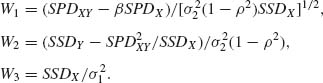
Or, equivalently,
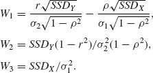
From (2.13.9) one obtains that
(2.13.10) ![]()
An immediate conclusion is that, when ρ = 0,
(2.13.11) ![]()
This result has important applications in testing the significance of the correlation coefficient. Generally, one can prove that the p.d.f. of r is
(2.13.12) ![]()
2.14 EXPONENTIAL TYPE FAMILIES
A family of distribution ![]() , having density functions f(x;θ) with respect to some σ–finite measure μ, is called a k–parameter exponential type family if
, having density functions f(x;θ) with respect to some σ–finite measure μ, is called a k–parameter exponential type family if
(2.14.1) ![]()
-∞ < x < ∞, θ ![]() Θ. Here ψi(θ), i = 1, …, k are functions of the parameters and Ui (x), i = 1, …, k are functions of the observations.
Θ. Here ψi(θ), i = 1, …, k are functions of the parameters and Ui (x), i = 1, …, k are functions of the observations.
In terms of the parameters ψ = (ψ1, …, ψk)′ and the statistics U = (U1 (x), …, Uk (x))′, the p.d.f of a k–parameter exponential type distribution can be written as
where K(ψ) = -log A*(ψ). Notice that h*(U(x)) > 0 for all x on the support set of ![]() , namely the closure of the smallest Borel set S, such that Pψ{S} = 1 for all ψ. If h*(U(x)) does not depend on ψ, we say that the exponential type family
, namely the closure of the smallest Borel set S, such that Pψ{S} = 1 for all ψ. If h*(U(x)) does not depend on ψ, we say that the exponential type family ![]() is regular. Define the domain of convergence to be
is regular. Define the domain of convergence to be
(2.14.3) ![]()
The family ![]() is called full if the parameter space Ω coincides with Ω*. Formula (2.14.2) is called the canonical form of the p.d.f.; ψ are called the canonical (or natural) parameters. The statistics Ui (x)(i = 1, …, k) are called canonical statistics. The family
is called full if the parameter space Ω coincides with Ω*. Formula (2.14.2) is called the canonical form of the p.d.f.; ψ are called the canonical (or natural) parameters. The statistics Ui (x)(i = 1, …, k) are called canonical statistics. The family ![]() is said to be of order k if (1, ψ1, …, ψk) are linearly independent functions of θ. Indeed if, for example, ψk =
is said to be of order k if (1, ψ1, …, ψk) are linearly independent functions of θ. Indeed if, for example, ψk =  , for some α0, …, αk – 1, which are not all zero, then by the reparametrization to
![]()
we reduce the number of canonical parameters to k – 1. If (1, ψ1, …, ψk) are linearly independent, the exponential type family is called minimal.
The following is an important theorem.
Theorem 2.14.1 If Equation (2.14.2) is a minimal representation then
For proof, see Brown (1986, p. 19).
Let
(2.14.4) ![]()
Accordingly, λ (ψ) = exp {K(ψ)} or K(ψ) = log λ (ψ). λ (ψ) is an analytic function on the interior of Ω* (see Brown, 1986, p. 32). Thus, λ (ψ) can be differentiated repeatedly under the integral sign and we have for nonnegative integers li, such that  ,
,
(2.14.5) 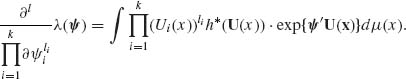
The m.g.f. of the canonical p.d.f. (2.14.2) is, for ψ in Ω*,
(2.14.6) 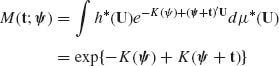
for t sufficiently close to 0. The logarithm of M(t;ψ), the cumulants generating function, is given here by
(2.14.7) ![]()
Accordingly,
(2.14.8) 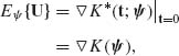
where ![]() denotes the gradient vector, i.e.,
denotes the gradient vector, i.e.,
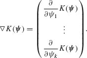
Similarly, the covariance matrix of U is
(2.14.9) ![]()
Higher order cumulants can be obtained by additional differentiation of K(ψ). We conclude this section with several comments.
2.15 APPROXIMATING THE DISTRIBUTION OF THE SAMPLE MEAN: EDGEWORTH AND SADDLEPOINT APPROXIMATIONS
Let X1, X2, …, Xn be i.i.d. random variables having a distribution, with all required moments existing.
2.15.1 Edgeworth Expansion
The Edgeworth Expansion of the distribution of Wn = ![]() , which is developed below, may yield more satisfactory approximation than that of the normal. This expansion is based on the following development.
, which is developed below, may yield more satisfactory approximation than that of the normal. This expansion is based on the following development.
The p.d.f. of the standard normal distribution, ![]() (x), has continuous derivatives of all orders everywhere. By repeated differentiation we obtain
(x), has continuous derivatives of all orders everywhere. By repeated differentiation we obtain
(2.15.1) 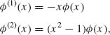
and generally, for j ≥ 1,
(2.15.2) ![]()
where Hj(x) is a polynomial of order j, called the Chebychev–Hermite polynomial. These polynomials can be obtained recursively by the formula, j ≥ 2,
(2.15.3) ![]()
where H0(x) ≡ 1 and H1(x) = x.
From this recursive relation one can prove by induction, that an even order polynomial H2m(x), m ≥ 1, contains only terms with even powers of x, and an odd order polynomial, H2m + 1(x), n ≥ 0, contains only terms with odd powers of x. One can also show that
(2.15.4) ![]()
Furthermore, one can prove the orthogonality property
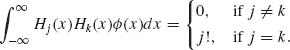
Thus, the system {Hj(x), j = 0, 1, …} of Chebychev–Hermite polynomials constitutes an orthogonal base for representing every continuous, integrable function f(x) as
(2.15.6) 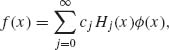
where, according to (2.15.5),
(2.15.7) ![]()
In particular, if f(x) is a p.d.f. of an absolutely continuous distribution, having all moments, then, for all -∞ < x < ∞,
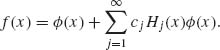
Moreover,
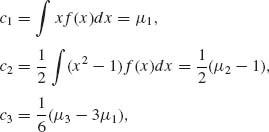
etc. If X is a standardized random variable, i.e., μ1 = 0 and μ2 = ![]() = 1, then its p.d.f. f(x) can be approximated by the formula
= 1, then its p.d.f. f(x) can be approximated by the formula
which involves the first four terms of the expansion (2.15.8). For the standardized sample mean ![]() ,
,
(2.15.10) ![]()
and
(2.15.11) ![]()
where β1 and β2 are the coefficients of skewness and kurtosis.
The same type of approximation with additional terms is known as the Edgeworth expansion. The Edgeworth approximation to the c.d.f. of Wn is
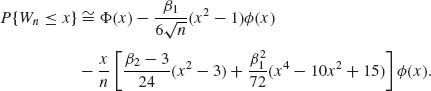
The remainder term in this approximation is of a smaller order of magnitude than ![]() , i.e.,
, i.e., ![]() . One can obviously expand the distribution with additional terms to obtain a higher order of accuracy. Notice that the standard CLT can be proven by taking limits, as n → ∞, of the two sides of (2.15.12).
. One can obviously expand the distribution with additional terms to obtain a higher order of accuracy. Notice that the standard CLT can be proven by taking limits, as n → ∞, of the two sides of (2.15.12).
We conclude this section with the remark that Equation (2.15.9) could serve to approximate the p.d.f. of any standardized random variable, having a continuous, integrable p.d.f., provided the moments exist.
2.15.2 Saddlepoint Approximation
As before, let X1, …, Xn be i.i.d. random variables having a common density f(x). We wish to approximate the p.d.f of ![]() . Let M(t) be the m.g.f. of t, assumed to exist for all t in (-∞, t0), for some 0 < t0 < ∞. Let K(t) = log M(t) be the corresponding cumulants generating function.
. Let M(t) be the m.g.f. of t, assumed to exist for all t in (-∞, t0), for some 0 < t0 < ∞. Let K(t) = log M(t) be the corresponding cumulants generating function.
We construct a family of distributions ![]() = {f(x, ψ): -∞ < ψ < t0} such that
= {f(x, ψ): -∞ < ψ < t0} such that
(2.15.13) ![]()
The family ![]() is called an exponential conjugate to f(x). Notice that f(x; 0) = f(x), and that
is called an exponential conjugate to f(x). Notice that f(x; 0) = f(x), and that ![]() .
.
Using the inversion formula for Laplace transforms, one gets the relationship
where ![]() denotes the p.d.f. of the sample mean of n i.i.d. random variables from f(x; ψ). The p.d.f.
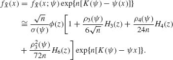
denotes the p.d.f. of the sample mean of n i.i.d. random variables from f(x; ψ). The p.d.f. ![]() is now approximated by the expansion (2.15.9) with additional terms, and its modification for the standardized mean Wn. Accordingly,
is now approximated by the expansion (2.15.9) with additional terms, and its modification for the standardized mean Wn. Accordingly,
where ![]() (z) is the p.d.f. of
(z) is the p.d.f. of ![]() , and ρ4(ψ) = K(4)(ψ)/(K(2)(ψ))2. Furthermore, μ (ψ) = K′(ψ) and σ2(ψ) = K(2)(ψ).
, and ρ4(ψ) = K(4)(ψ)/(K(2)(ψ))2. Furthermore, μ (ψ) = K′(ψ) and σ2(ψ) = K(2)(ψ).
The objective is to approximate ![]() . According to (2.15.14) and (2.15.15), we approximate
. According to (2.15.14) and (2.15.15), we approximate ![]() by
by
The approximation is called a saddlepoint approximation if we substitute in (2.15.16) ψ = ![]() , where ψ is a point in (-∞, t0) that maximizes f(x; ψ). Thus,
, where ψ is a point in (-∞, t0) that maximizes f(x; ψ). Thus, ![]() is the root of the equation
is the root of the equation
![]()
As we have seen in Section 2.14, K(ψ) is strictly convex in the interior of (−∞, t0). Thus, K′(ψ) is strictly increasing in (-∞, t0). Thus, if ![]() exists then it is unique. Moreover, the value of z at ψ =
exists then it is unique. Moreover, the value of z at ψ = ![]() is z = 0. It follows that the saddlepoint approximation is
is z = 0. It follows that the saddlepoint approximation is
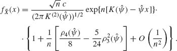
The coefficient c is introduced on the right–hand side of (2.15.17) for normalization. A lower order approximation is given by the formula
The saddelpoint approximation to the tail of the c.d.f., i.e., ![]() is known to yield very accurate results. There is a famous Lugannani–Rice (1980) approximation to this tail probability. For additional reading, see Barndorff–Nielson and Cox (1979), Jensen (1995), Field and Ronchetti (1990), Reid (1988), and Skovgaard (1990).
is known to yield very accurate results. There is a famous Lugannani–Rice (1980) approximation to this tail probability. For additional reading, see Barndorff–Nielson and Cox (1979), Jensen (1995), Field and Ronchetti (1990), Reid (1988), and Skovgaard (1990).
PART II: EXAMPLES
Example 2.1. In this example we provide a few important results on the distributions of sums of independent random variables.
A. Binomial
If X1 and X2 are independent, X1 ∼ B(N1, θ), X2 ∼ B(N2, θ), then X1 + X2 ∼ B(N1 + N2, θ). It is essential that the binomial distributions of X1 and X2 will have the same value of θ. The proof is obtained by multiplying the corresponding m.g.f.s.
B. Poisson
If X1 ∼ P(λ1) and X2 ∼ P(λ2) then, under independence, X1 + X2 ∼ P(λ1 + λ2).
C. Negative–Binomial
If X1 ∼ NB(ψ, ν1) and X2 ∼ NB(ψ, ν2) then, under independence, X1 + X2 ∼ NB(ψ, ν1 + ν2). It is essential that the two distributions will depend on the same ψ.
D. Gamma
If X1 ∼ G(λ, ν1) and X2 ∼ G(λ, ν2) then, under independence, X1 + X2 ∼ G(λ, ν1 + ν2). It is essential that the two values of the parameter λ will be the same. In particular,
![]()
for all ν1, ν2 = 1, 2, …; where ![]() [νi], i = 1, 2, denote two independent χ2–random variables with ν1 and ν2 degrees of freedom, respectively. This result has important applications in the theory of normal regression analysis.
[νi], i = 1, 2, denote two independent χ2–random variables with ν1 and ν2 degrees of freedom, respectively. This result has important applications in the theory of normal regression analysis.
E. Normal
If X1 ∼ N(μ, ![]() ) and X2 ∼ N(μ2,
) and X2 ∼ N(μ2, ![]() ) and if X1 and X2 are independent, then X1 + X2 ∼ N(μ1 + μ2,
) and if X1 and X2 are independent, then X1 + X2 ∼ N(μ1 + μ2, ![]() +
+![]() ). A generalization of this result to the case of possible dependence is given later.
). A generalization of this result to the case of possible dependence is given later. ![]()
Example 2.2 Using the theory of transformations, the following important result is derived. Let X1 and X2 be independent,
![]()
then the ratio R = X1/(X1 + X2) has a beta distribution, β (ν1, ν2), independent of λ. Furthermore, R and T = X1 + X2 are independent. Indeed, the joint p.d.f. of X1 and X2 is
![]()
Consider the transformation
![]()
The Jacobian of this transformation is J(x1, t) = 1. The joint p.d.f. of X1 and T is then
![]()
We have seen in the previous example that T = X1 + X2 ∼ G(λ, ν1 + ν2). Thus, the marginal p.d.f. of T is
![]()
Making now the transformation
![]()
we see that the Jacobian is J(r, t) = t. Hence, from (2.4.8) and (2.4.9) the joint p.d.f. of r and t is, for 0 ≤ r ≤ 1 and 0 ≤ t < ∞,
![]()
This proves that R ∼ β (ν1, ν2) and that R and T are independent. ![]()
Example 2.3. Let (X, λ) be random variables, such that the conditional distribution of X given λ is Poisson with p.d.f.
![]()
and λ ∼ G(ν, Λ). Hence, the marginal p.d.f. of X is
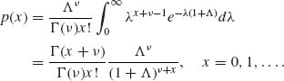
Let ![]() . Then
. Then ![]() . Thus, X ∼ NB(ψ, ν), and we get
. Thus, X ∼ NB(ψ, ν), and we get
But,
![]()
Hence,
![]()
where G(1, k + 1) and G(1, ν) are independent.
Let R = ![]() . According to Example 2.2,
. According to Example 2.2,
![]()
But U ∼ ![]() ; hence,
; hence,
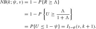
![]()
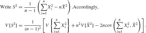
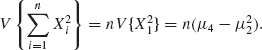
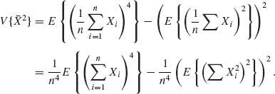
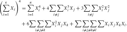
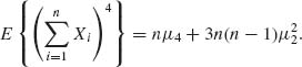
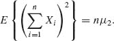
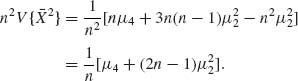
Example 2.4. Let X1, …, Xn be i.i.d. random variables. Consider the linear and the quadratic functions
We compute first the variance of S2. Notice first that S2 does not change its value if we substitute ![]() = Xi – μ1 for Xi (i = 1, …, n). Thus, we can assume that μ1 = 0 and all moments are central moments.
= Xi – μ1 for Xi (i = 1, …, n). Thus, we can assume that μ1 = 0 and all moments are central moments.
Now, since X1, …, Xn are i.i.d.,
Also,
According to Table 2.3,
![]()
Thus,
Therefore, since μ1 = 0, the independence implies that
Also,
Thus,
At this stage we have to compute
From Table (2.3), (2)(1)2 = [4] + 2[31] + [22] + [212]. Hence,
and
Therefore,
Finally, substituting these terms we obtain
![]()
![]()
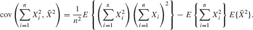
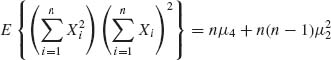
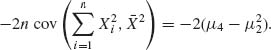
Example 2.5. We develop now the formula for the covariance of ![]() and S2.
and S2.
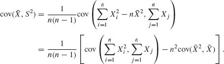
First,
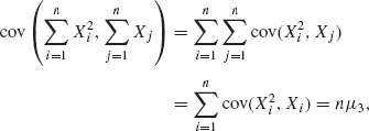
since the independence of Xi and Xj for all i ≠ j implies that cov(![]() , Xj) = 0. Similarly,
, Xj) = 0. Similarly,
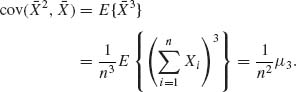
Thus, we obtain
![]()
Finally, if the distribution function F(x) is symmetric about zero, μ3 = 0, and cov(![]() , S2) = 0.
, S2) = 0. ![]()
Example 2.6. The number of items, N, demanded in a given store during one week is a random variable having a Negative–Binomial distribution NB(ψ, ν); 0 < ψ < 1 and 0 < ν < ∞. These items belong to k different classes. Let X = (X1, …, Xk)′ denote a vector consisting of the number of items of each class demanded during the week. These are random variables such that  and the conditional distribution of (X1, …, Xk) given N is the multinomial M(N, θ), where θ = (θ1, …, θk) is the vector of probabilities; 0 < θi < 1,
 ![]() . If we observe the X vectors over many weeks and construct the proportional frequencies of the X values in the various classes, we obtain an empirical distribution of these vectors. Under the assumption that the model and its parameters remain the same over the weeks we can fit to that empirical distribution the theoretical marginal distribution of X. This marginal distribution is obtained in the following manner.
. If we observe the X vectors over many weeks and construct the proportional frequencies of the X values in the various classes, we obtain an empirical distribution of these vectors. Under the assumption that the model and its parameters remain the same over the weeks we can fit to that empirical distribution the theoretical marginal distribution of X. This marginal distribution is obtained in the following manner.
The m.g.f. of the conditional multinomial distribution of X* = (X1, …, Xk – 1)′ given N is
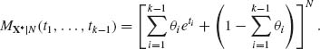
Hence, the m.g.f. of the marginal distribution of X* is
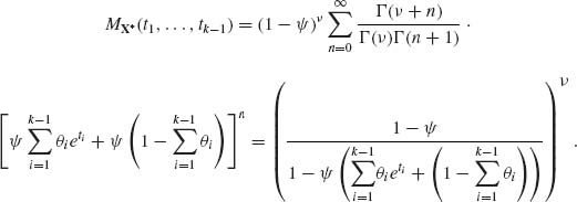
Or
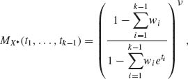
where
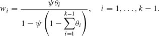
This proves that X* has the multivariate Negative–Binomial distribution. ![]()
Example 2.7. Consider a random variable X having a normal distribution, N(ξ, σ2). Let Φ(u) be the standard normal c.d.f. The transformed variable Y = Φ(X) is of interest in various problems of statistical inference in the fields of reliability, quality control, biostatistics, and others. In this example we study the first two moments of Y.
In the special case of ξ = 0 and σ2 = 1, since Φ(u) is the c.d.f. of X, the above transformation yields a rectangular random variable, i.e., Y ∼ R(0, 1). In this case, obviously E{Y} = 1/2 and V{Y} = 1/12. In the general case, we have according to the law of the iterated expectation
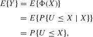
where U ∼ N(0, 1), U and X are independent. Moreover, according to (2.7.7), U – X∼ N(–ξ, 1 + σ2). Therefore,
![]()
In order to determine the variance of Y we observe first that, if U1, U2 are independent random variables identically distributed like N(0, 1), then P{U1 ≤ x, U2 ≤ x} = Φ2(x) for all -∞ < x < ∞. Thus,
![]()
where U1, U2 and X are independent and Ui ∼ N(0, 1), i = 1, 2, U1 – X and U2 – X have a joint bivariate normal distribution with mean vector (–ξ, –ξ) and covariance matrix
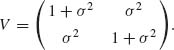
Hence,
![]()
Finally,
![]()
Generally, the nth moment of Y can be determined by the n–variate multinormal c.d.f. ![]() , where the correlation matrix R has off–diagonal elements Rij = σ2/(1 + σ2), for all k ≠ j. We do not treat here the problem of computing the standard k–variate multinormal c.d.f. Computer routines are available for small values of k. The problem of the numerical evaluation is generally difficult. Tables are available for the bivariate and the trivariate cases. For further comments on this issue see Johnson and Kotz (1972, pp. 83–132).
, where the correlation matrix R has off–diagonal elements Rij = σ2/(1 + σ2), for all k ≠ j. We do not treat here the problem of computing the standard k–variate multinormal c.d.f. Computer routines are available for small values of k. The problem of the numerical evaluation is generally difficult. Tables are available for the bivariate and the trivariate cases. For further comments on this issue see Johnson and Kotz (1972, pp. 83–132). ![]()
Example 2.8. Let X1, X2, …, Xn be i.i.d. N(0, 1) r.v.s. The sample variance is defined as
![]()
Let Q = Σ (Xi – ![]() )2. Define the matrix J = 11′, where 1′ = (1, …, 1) is a vector of ones. Let A =
)2. Define the matrix J = 11′, where 1′ = (1, …, 1) is a vector of ones. Let A = ![]() , and Q = X′AX. It is easy to verify that A is an idempotent matrix. Indeed,
, and Q = X′AX. It is easy to verify that A is an idempotent matrix. Indeed,
![]()
The rank of A is r = n – 1. Thus, we obtained that S2 ![]() .
. ![]()
Example 2.9. Let X1, …, Xn be i.i.d. random variables having a N(ξ, σ2) distribution. The sample mean is ![]() and the sample variance is S2
and the sample variance is S2 ![]() . In Section 2.5 we showed that if the distribution of the Xs is symmetric, then
. In Section 2.5 we showed that if the distribution of the Xs is symmetric, then ![]() and S2 are uncorrelated. We prove here the stronger result that, in the normal case,
and S2 are uncorrelated. We prove here the stronger result that, in the normal case, ![]() and S2 are independent. Indeed,
and S2 are independent. Indeed,
![]()
is distributed like N(0, I). Moreover, S2 ![]() . But,
. But,
![]()
This implies the independence of ![]() and S2.
and S2. ![]()
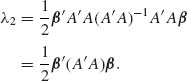
Example 2.10. Let X be a k–dimensional random vector having a multinormal distribution N(Aβ, σ2I), where A is a k × r matrix of constants, β is an r × 1 vector; 1 ≤ r ≤ k, 0 < σ2 < ∞. We further assume that rank (A) = r, and the parameter vector β is unknown. Consider the vector ![]() that minimizes the squared–norm ||X – Aβ} ||2, where ||X||2 =
that minimizes the squared–norm ||X – Aβ} ||2, where ||X||2 = ![]() . Such a vector
. Such a vector ![]() is called the least–squares estimate of β. The vector
is called the least–squares estimate of β. The vector ![]() is determined so that
is determined so that
![]()
That is, A![]() is the orthogonal projection of X on the subspace generated by the column vectors of A. Thus, the inner product of (X – A
is the orthogonal projection of X on the subspace generated by the column vectors of A. Thus, the inner product of (X – A![]() ) and A
) and A![]() should be zero. This implies that
should be zero. This implies that
![]()
The matrix A′A is nonsingular, since A is of full rank. Substituting ![]() in the expressions for Q1 and Q2, we obtain
in the expressions for Q1 and Q2, we obtain
![]()
and
![]()
We prove now that these quadratic forms are independent. Both
![]()
are idempotent. The rank of B1 is k – r and that of B2 is r. Moreover,
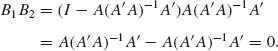
Thus, the conditions of Theorem 2.9.2 are satisfied and Q1 is independent of Q2. Moreover, Q1 ∼ σ2 χ2[x –r; λ1] and Q2 ∼ σ2χ2[r;λ2] where
![]()
and
![]()
Example 2.11. Let X1, …, Xn be i.i.d. random variables from a rectangular R(0, 1) distribution. The density of the ith order statistic is then
![]()
0≤ x ≤ 1. The p.d.f. of the sample median, for n = 2m + 1, is in this case
![]()
The p.d.f. of the sample range is the β (n – 1, 2) density
![]()
These results can be applied to test whether a sample of n observation is a realization of i.i.d. random variables having a specified continuous distribution, F(x), since Y = F(Y) ∼ R(0, 1). ![]()
Example 2.12. Let X1, X2, …, Xn be i.i.d. random variables having a common exponential distribution E(λ), 0 < λ < ∞. Let X(1) < X(2) < … < X(n) be the corresponding order statistic. The density of X(1) is
![]()
The joint density of X(1) and X(2) is
![]()
Let U = X(2)–X(1). The joint density of X(1) and U is
![]()
and 0 < u < ∞. Notice that fX(1),U(x, u) = fX(1)(x)· fU(u). Thus X(1) and U are independent, and U is distributed like the minimum of (n – 1) i.i.d. E(λ) random variables. Similarly, by induction on k = 2, 3, …, n, if Uk = X(k) – X(k-1) then X(k-1) and Uk are independent and Uk ∼ E(λ (n – k + 1)). Thus, since X(k) = X(1) + U2 + … + Uk, E{X(k)} =  and
and 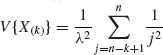 , for all k ≥ 1.
 ![]()
Example 2.13. Let X ∼ N(μ, σ2), -∞ < μ < ∞, 0 < σ2 < ∞. The p.d.f. of X is
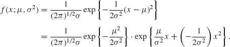
Let h(x) = ![]() , U1 (x) = x, and U2 (x) = x2. We can write f(x;μ, σ2) as a two–parameter exponential type family. By making the reparametrization (μ, σ2) → (ψ1, ψ2), the parameter space Θ = {(μ, σ2): -∞ < μ < ∞, 0 < σ2 < ∞} is transformed to the parameter space
, U1 (x) = x, and U2 (x) = x2. We can write f(x;μ, σ2) as a two–parameter exponential type family. By making the reparametrization (μ, σ2) → (ψ1, ψ2), the parameter space Θ = {(μ, σ2): -∞ < μ < ∞, 0 < σ2 < ∞} is transformed to the parameter space
![]()
In terms of (ψ1, ψ2) the density of X can be written as
![]()
where h(x) = 1/![]() and
and
![]()
The p.d.f. of the standard normal distribution is obtained by substituting ψ1 = 0, ψ2 = ![]() .
. ![]()
Example 2.14. A simple example of a curved exponential family is
![]()
In this case,
![]()
with ψ2 = ![]() . ψ1 and ψ2 are linearly independent. The rank is k = 2 but
. ψ1 and ψ2 are linearly independent. The rank is k = 2 but
![]()
The dimension of Ω* is 1.
The following example shows a more interesting case of a regular exponential family of order k = 3. ![]()
Example 2.15. We consider here a model that is well known as the Model II of Analysis of Variance. This model will be discussed later in relation to the problem of estimation and testing variance components.
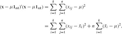
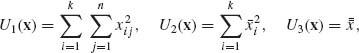
We are given n · k observations on random variables Xij (i = 1, …, k; j = 1, …, n). These random variables represent the results of an experiment performed in k blocks, each block containing n trials. In addition to the random component representing the experimental error, which affects the observations independently, there is also a random effect of the blocks. This block effect is the same on all the observations within a block, but is independent from one block to another. Accordingly, our model is
![]()
where eij are i.i.d. like N(0, σ2) and ai are i.i.d. like N(0, τ2).
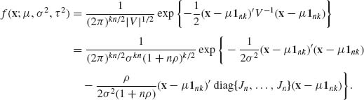
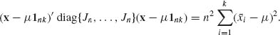
We determine now the joint p.d.f. of the vector X = (X11, …, X1n, X21, …, X2n, …, Xk1, …, Xkn)′. The conditional distribution of X given a = (a1, …, ak)′ is the multinormal N(μ 1nk + ξ (a), σ2Ink), where ξ}′(a) = (a1 1′n, a2 1′n, …, ak 1′n). Hence, the marginal distribution of X is the multinormal N(ξ 1nk, V), where the covariance matrix V is given by a matrix composed of k equal submatrices along the main diagonal and zeros elsewhere. That is, if Jn = 1n 1′n is an n × n matrix of 1s,
![]()
The determinant of V is (σ2)kn|In + ρ Jn |k, where ρ = τ2/σ2. Moreover, let H be an orthogonal matrix whose first row vector is ![]() . Then,
. Then,
![]()
Hence, |V| = σ2nk(1 + nρ)k. The inverse of V is
![]()
where (In + ρ Jn)-1 = In – (ρ/(1 + nρ))Jn.
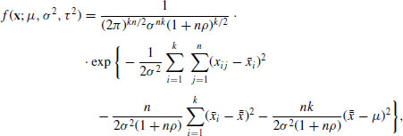
Accordingly, the joint p.d.f. of X is
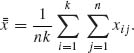
Furthermore,
where ![]() . Similarly,
. Similarly,
Substituting these terms we obtain,
where
Define,
and make the reparametrization
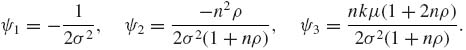
The joint p.d.f. of X can be expressed then as
![]()
The functions U1 (x), U2 (x), and U3 (x) as well as ψ1(θ), ψ2(θ), and ψ3(θ) are linearly independent. Hence, the order is k = 3, and the dimension of Ω* is d = 3. ![]()
Example 2.16. Let X1, …, Xn be i.i.d. random variables having a common gamma distribution G(λ, ν), 0 < λ, ν < ∞. For this distribution β1 = 2ν and β2 = 6ν.
The sample mean ![]() n is distributed like
n is distributed like ![]() . The standardized mean is
. The standardized mean is ![]() . The exact c.d.f. of Wn is
. The exact c.d.f. of Wn is
![]()
On the other hand, the Edgeworth approximation is
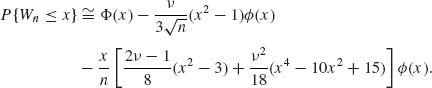
In the following table, we compare the exact distribution of Wn with its Edgeworth expansion for the case of ν = 1, n = 10, and n = 20. We see that for n = 20 the Edgeworth expansion yields a very good approximation, with a maximal relative error of -4.5% at x = -2. At x = -1.5 the relative error is 0.9%. At all other values of x the relative error is much smaller.
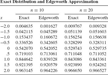
![]()
Example 2.17. Let X1, …, Xn be i.i.d. distributed as G(λ, ν). ![]() . Accordingly,
. Accordingly,
![]()
The cumulant generating function of G(λ, ν) is
![]()
Thus,
![]()
and
![]()
Accordingly, ![]() = λ – ν /x and
= λ – ν /x and
![]()
exp{n[K(![]() ) –
) – ![]() x]} = exp{nν –nλx} ·
x]} = exp{nν –nλx} · ![]() . It follows from Equation (2.15.18) that the saddlepoint approximation is
. It follows from Equation (2.15.18) that the saddlepoint approximation is
![]()
If we substitute in the exact formula the Stirling approximation, ![]() , we obtain the saddlepoint approximation.
, we obtain the saddlepoint approximation. ![]()