
CHAPTER 6
Confidence and Tolerance Intervals
PART I: THEORY
6.1 GENERAL INTRODUCTION
When θ is an unknown parameter and an estimator ![]() is applied, the precision of the estimator
is applied, the precision of the estimator ![]() can be stated in terms of its sampling distribution. With the aid of the sampling distribution of an estimator we can determine the probability that the estimator θ lies within a prescribed interval around the true value of the parameter θ. Such a probability is called confidence (or coverage) probability. Conversely, for a preassigned confidence level, we can determine an interval whose limits depend on the observed sample values, and whose coverage probability is not smaller than the prescribed confidence level, for all θ. Such an interval is called a confidence interval. In the simple example of estimating the parameters of a normal distribution N(μ, σ2), a minimal sufficient statistic for a sample of size n is (
can be stated in terms of its sampling distribution. With the aid of the sampling distribution of an estimator we can determine the probability that the estimator θ lies within a prescribed interval around the true value of the parameter θ. Such a probability is called confidence (or coverage) probability. Conversely, for a preassigned confidence level, we can determine an interval whose limits depend on the observed sample values, and whose coverage probability is not smaller than the prescribed confidence level, for all θ. Such an interval is called a confidence interval. In the simple example of estimating the parameters of a normal distribution N(μ, σ2), a minimal sufficient statistic for a sample of size n is (![]() n,
n, ![]() ). We wish to determine an interval (μ (
). We wish to determine an interval (μ (![]() n,
n, ![]() ),
), ![]() (
(![]() n,
n, ![]() )) such that
)) such that
for all μ, σ. The prescribed confidence level is 1 − α and the confidence interval is (μ, ![]() ). It is easy to prove that if we choose the functions
). It is easy to prove that if we choose the functions
(6.1.2) 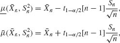
then (6.1.1) is satisfied. The two limits of the confidence interval (μ, ![]() ) are called the lower and upper confidence limits. Confidence limits for the variance σ2 in the normal case can be obtained from the sampling distribution of
) are called the lower and upper confidence limits. Confidence limits for the variance σ2 in the normal case can be obtained from the sampling distribution of ![]() . Indeed, since
. Indeed, since ![]() . The lower and upper confidence limits for σ2 are given by
. The lower and upper confidence limits for σ2 are given by
(6.1.3) 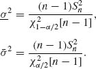
A general method to derive confidence intervals in parametric cases is given in Section 6.2. The theory of optimal confidence intervals is developed in Section 6.3 in parallel to the theory of optimal testing of hypotheses. The theory of tolerance intervals and regions is discussed in Section 6.4. Tolerance intervals are estimated intervals of a prescribed probability content according to the unknown parent distribution. One sided tolerance intervals are often applied in engineering designs and screening processes as illustrated in Example 6.1.
Distribution free methods, based on the properties of order statistics, are developed in Section 6.5. These methods yield tolerance intervals for all distribution functions having some general properties (log–convex for example). Section 6.6 is devoted to the problem of determining simultaneous confidence intervals for several parameters. In Section 6.7, we discuss two–stage and sequential sampling to obtain fixed–width confidence intervals.
6.2 THE CONSTRUCTION OF CONFIDENCE INTERVALS
We discuss here a more systematic method of constructing confidence intervals.
Let ![]() = {F(x;θ), θ
= {F(x;θ), θ ![]() Θ } be a parametric family of d.f.s. The parameter θ is real or vector valued. Given the observed value of X, we construct a set S(X) in Θ such that
Θ } be a parametric family of d.f.s. The parameter θ is real or vector valued. Given the observed value of X, we construct a set S(X) in Θ such that
(6.2.1) ![]()
S(X) is called a confidence region for θ at level of confidence 1 − α. Note that the set S(X) is a random set, since it is a function of X. For example, consider the multinormal N(θ, I) case. We know that (X − θ)′ (X − θ) is distributed like χ2[k], where k is the dimension of X. Thus, define
(6.2.2) ![]()
It follows that, for all θ,
(6.2.3) ![]()
Accordingly, S(X) is a confidence region. Note that if the problem, in this multinormal case, is to test the simple hypothesis H0: θ = θ0 against the composite alternative H1: θ ≠ θ0 we would apply the test statistic
(6.2.4) ![]()
and reject H0 whenever T(θ0) ≥ ![]() [k]. This test has size α. If we define the acceptance region for H0 as the set
[k]. This test has size α. If we define the acceptance region for H0 as the set
(6.2.5) ![]()
then H0 is accepted if X ![]() A (θ0). The structures of A(θ0) and S(X) are similar. In A(θ0), we fix θ at θ0 and vary X, while in S(X) we fix X and vary θ. Thus, let
A (θ0). The structures of A(θ0) and S(X) are similar. In A(θ0), we fix θ at θ0 and vary X, while in S(X) we fix X and vary θ. Thus, let ![]() = {A(θ);θ
= {A(θ);θ ![]() Θ } be a family of acceptance regions for the above testing problem, when θ varies over all the points in Θ. Such a family induces a family of confidence sets
Θ } be a family of acceptance regions for the above testing problem, when θ varies over all the points in Θ. Such a family induces a family of confidence sets ![]() = {S(X):X
= {S(X):X ![]()
![]() } according to the relation
} according to the relation
In such a manner, we construct generally confidence regions (or intervals). We first construct a family of acceptance regions, ![]() for testing H0: θ = θ0 against H1: θ ≠ θ0 at level of significance α. From this family, we construct the dual family
for testing H0: θ = θ0 against H1: θ ≠ θ0 at level of significance α. From this family, we construct the dual family ![]() of confidence regions. We remark here that in cases of a real parameter θ we can consider one–sided hypotheses H0: θ ≤ θ0 against H1: θ > θ0; or H0: θ ≥ θ0 against H1: θ < θ0. The corresponding families of acceptance regions will induce families of one–sided confidence intervals (−∞,
of confidence regions. We remark here that in cases of a real parameter θ we can consider one–sided hypotheses H0: θ ≤ θ0 against H1: θ > θ0; or H0: θ ≥ θ0 against H1: θ < θ0. The corresponding families of acceptance regions will induce families of one–sided confidence intervals (−∞, ![]() (X)) or (θ(X), ∞), respectively.
(X)) or (θ(X), ∞), respectively.
6.3 OPTIMAL CONFIDENCE INTERVALS
In the previous example, we have seen two different families of lower confidence intervals, one of which was obviously inefficient. We introduce now the theory of uniformly most accurate (UMA) confidence intervals. According to this theory, the family of lower confidence intervals θα in the above example is optimal.
Definition. A lower confidence limit for θ, θ(X) is called UMA if, given any other lower confidence limit θ* (X),
(6.3.1) ![]()
for all θ′ < θ, and all θ.
That is, although both the θ(X) and θ* (X) are smaller than θ with confidence probability (1 − α), the probability is larger that the UMA limit θ (X) is closer to the true value θ than that of θ* (X). Whenever a size α uniformly most powerful (UMP) test exists for testing the hypothesis H0: θ ≤ θ0 against H1: θ > θ0, then a UMA (1 − α)–lower confidence limit exists. Moreover, one can obtain the UMA lower confidence limit from the UMP test function according to relationship (6.2.6). The proof of this is very simple and left to the reader. Thus, as proven in Section 4.3, if the family of d.f.s ![]() is a one–parameter MLR family, the UMP test of size α, of H0: θ ≤ θ0 against H1: θ > θ1 is of the form
is a one–parameter MLR family, the UMP test of size α, of H0: θ ≤ θ0 against H1: θ > θ1 is of the form
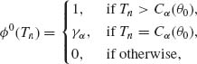
where Tn is the minimal sufficient statistic. Accordingly, if Tn is a continuous random variable, the family of acceptance intervals is
(6.3.3) ![]()
The corresponding family of (1 − α)–lower confidence limits is
(6.3.4) ![]()
In the discrete monotone likelihood ratio (MLR) case, we reduce the problem to that of a continuous MLR by randomization, as specified in (6.3.2). Let Tn be the minimal sufficient statistic and, without loss of generality, assume that Tn assumes only the nonnegative integers. Let Hn(t; θ) be the cumulative distribution function (c.d.f.) of Tn under θ. We have seen in Chapter 4 that the critical level of the test (6.3.2) is
(6.3.5) ![]()
Moreover, since the distributions are MLR, Cα (θ) is a nondecreasing function of θ. In the continuous case, we determined the lower confidence limit θα as the root, θ, of the equation Tn = Cα (θ). In the discrete case, we determine θα as the root, θ, of the equation
where R is a random variable independent of Tn and having a rectangular distribution R(0, 1). We can express Equation (6.3.6) in the form
(6.3.7) ![]()
If UMP tests do not exist we cannot construct UMA confidence limits. However, we can define UMA–unbiased or UMA–invariant confidence limits and apply the theory of testing hypotheses to construct such limits. Two–sided confidence intervals (θα (X), ![]() α (X)) should satisfy the requirement
α (X)) should satisfy the requirement
A two–sided (1 − α) confidence interval (θα (X), ![]() α (X)) is called UMA if, subject to (6.3.8), it minimizes the coverage probabilities
α (X)) is called UMA if, subject to (6.3.8), it minimizes the coverage probabilities
(6.3.9) ![]()
In order to obtain UMA two–sided confidence intervals, we should construct a UMP test of size α of the hypothesis H0: θ = θ0 against H1: θ ≠ θ0. Such a test generally does not exist. However, we can construct a UMP–unbiased (UMPU) test of such hypotheses (in cases of exponential families) and derive then the corresponding confidence intervals.
A confidence interval of level 1 − α is called unbiased if, subject to (6.3.8), it satisfies
(6.3.10) ![]()
Confidence intervals constructed on the basis of UMPU tests are UMAU (uniformly most accurate unbiased) ones.
6.4 TOLERANCE INTERVALS
Tolerance intervals can be described in general terms as estimated prediction intervals for future realization(s) of the observed random variables. In Example 6.1, we discuss such an estimation problem and illustrate a possible solution. Consider a sequence X1, X2, … of independent and identically distributed (i.i.d.) random variables having a common distribution F(x;θ), θ ![]() Θ. A p–content prediction interval for a possible realization of X, when θ is known, is an interval (lp(θ), up(θ)) such that Pθ [X
Θ. A p–content prediction interval for a possible realization of X, when θ is known, is an interval (lp(θ), up(θ)) such that Pθ [X ![]() (lp(θ), up(θ ))] ≥ p. Such two–sided prediction intervals are not uniquely defined. Indeed, if F−1 (p;θ) is the pth quantile of F(x;θ) then for every 0 ≤
(lp(θ), up(θ ))] ≥ p. Such two–sided prediction intervals are not uniquely defined. Indeed, if F−1 (p;θ) is the pth quantile of F(x;θ) then for every 0 ≤ ![]() ≤ 1, lp = F−1(
≤ 1, lp = F−1(![]() (1-p);θ) and up = F−1 (1−(1−
(1-p);θ) and up = F−1 (1−(1−![]() )(1−p);θ) are lower and upper limits of a p–content prediction interval. Thus, p–content two–sided prediction intervals should be defined more definitely, by imposing further requirement on the location of the interval. This is, generally, done according to the specific problem under consideration. We will restrict attention here to one–sided prediction intervals of the form (−∞, F−1 (p;θ)] or [F−1(1−p;θ), ∞).
)(1−p);θ) are lower and upper limits of a p–content prediction interval. Thus, p–content two–sided prediction intervals should be defined more definitely, by imposing further requirement on the location of the interval. This is, generally, done according to the specific problem under consideration. We will restrict attention here to one–sided prediction intervals of the form (−∞, F−1 (p;θ)] or [F−1(1−p;θ), ∞).
When θ is unknown the limits of the prediction intervals are estimated. In this section, we develop the theory of such parametric estimation. The estimated prediction intervals are called tolerance intervals. Two types of tolerance intervals are discussed in the literature: p–content tolerance intervals (see Guenther, 1971), which are called also mean tolerance predictors (see Aitchison and Dunsmore, 1975); and (1 − α) level p–content intervals, also called guaranteed coverage tolerance intervals (Aitchison and Dunsmore, 1975; Guttman, 1970). p–Content one–sided tolerance intervals, say (−∞, Lp(Xn)), are determined on the basis of n sample values Xn = (X1, …, Xn) so that, if Y has the F(x;θ) distribution then
(6.4.1) ![]()
Note that
(6.4.2) ![]()
Thus, given the value of Xn, the upper tolerance limit Lp(Xn) is determined so that the expected probability content of the interval (−∞, Lp(Xn)] will be p. The (p, 1 − α) guaranteed coverage one–sided tolerance interval (−∞, Lα, p(Xn)) are determined so that
(6.4.3) ![]()
for all θ. In other words, Lα, p(Xn) is a (1 − α)–upper confidence limit for the pth quantile of the distribution F(x;θ). Or, with confidence level (1 − α), we can state that the expected proportion of future observations not exceeding Lα, p (Xn) is at least p. (p, 1 −α)–upper tolerance limits can be obtained in cases of MLR parametric families by substituting the (1 − α)–upper confidence limit ![]() α of θ in the formula of F−1(p;θ). Indeed, if
α of θ in the formula of F−1(p;θ). Indeed, if ![]() = {F(x;θ);θ
= {F(x;θ);θ ![]() Θ } is a family depending on a real parameter θ, and
Θ } is a family depending on a real parameter θ, and ![]() is MLR with respect to X, then the pth quantile, F−1(p;θ), is an increasing function of θ, for each 0 < p < 1. Thus, a one–sided p–content, (1 − α)–level tolerance interval is given by
is MLR with respect to X, then the pth quantile, F−1(p;θ), is an increasing function of θ, for each 0 < p < 1. Thus, a one–sided p–content, (1 − α)–level tolerance interval is given by
(6.4.4) ![]()
Moreover, if the upper confidence limit ![]() α (Xn) is UMA then the corresponding tolerance limit is a UMA upper confidence limit of F−1(p;θ). For this reason such a tolerance interval is called UMA. For more details, see Zacks (1971, p. 519).
α (Xn) is UMA then the corresponding tolerance limit is a UMA upper confidence limit of F−1(p;θ). For this reason such a tolerance interval is called UMA. For more details, see Zacks (1971, p. 519).
In Example 6.1, we derive the (β, 1 − α) guaranteed lower tolerance limit for the log–normal distribution. It is very simple in that case to determine the β–content lower tolerance interval. Indeed, if (![]() n,
n, ![]() ) are the sample mean and variance of the corresponding normal variables Yi = log Xi (i = 1, …, n) then
) are the sample mean and variance of the corresponding normal variables Yi = log Xi (i = 1, …, n) then
is such a β–content lower tolerance limit. Indeed, if a N(μ, σ) random variable Y is independent of (![]() n,
n, ![]() ) then
) then

since ![]() and
and ![]() . It is interesting to compare the β–content lower tolerance limit (6.4.5) with the (1 − α, β) guaranteed coverage lower tolerance limit (6.4.6). We can show that if β = 1 − α then the two limits are approximately the same in large samples.
. It is interesting to compare the β–content lower tolerance limit (6.4.5) with the (1 − α, β) guaranteed coverage lower tolerance limit (6.4.6). We can show that if β = 1 − α then the two limits are approximately the same in large samples.
6.5 DISTRIBUTION FREE CONFIDENCE AND TOLERANCE INTERVALS
Let ![]() be the class of all absolutely continuous distributions. Suppose that X1, …, Xn are i.i.d. random variables having a distribution F(x) in
be the class of all absolutely continuous distributions. Suppose that X1, …, Xn are i.i.d. random variables having a distribution F(x) in ![]() . Let X(1) ≤ ··· ≤ X(n) be the order statistics. This statistic is minimal sufficient. The transformed random variable Y = F(X) has a rectangular distribution on (0, 1). Let xp be the pth quantile of F(x), i.e., xp = F−1(p), 0 < p < 1. We show now that the order statistics X(i) can be used as (p, γ) tolerance limits, irrespective of the functional form of F(x). Indeed, the transformed random variables Y(i) = F(X(i)) have the beta distributions β (i, n − i + 1), i = 1, …, n. Accordingly,
. Let X(1) ≤ ··· ≤ X(n) be the order statistics. This statistic is minimal sufficient. The transformed random variable Y = F(X) has a rectangular distribution on (0, 1). Let xp be the pth quantile of F(x), i.e., xp = F−1(p), 0 < p < 1. We show now that the order statistics X(i) can be used as (p, γ) tolerance limits, irrespective of the functional form of F(x). Indeed, the transformed random variables Y(i) = F(X(i)) have the beta distributions β (i, n − i + 1), i = 1, …, n. Accordingly,
Therefore, a distribution free (p, γ) upper tolerance limit is the smallest X(j) satisfying condition (6.5.1). In other words, for any continuous distribution F(x), define
Then, the order statistic X(i0) is a (p, γ)–upper tolerance limit. We denote this by Lp, γ (X). Similarly, a distribution free (p, γ)–lower tolerance limit is given by
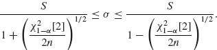
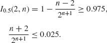
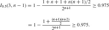
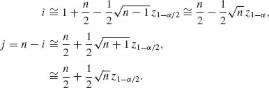
The upper and lower tolerance intervals given in (6.5.2) and (6.5.3) might not exist if n is too small. They could be applied to obtain distribution free confidence intervals for the mean, μ, of a symmetric continuous distribution. The method is based on the fact that the expected value, μ, and the median, F−1(0.5), of continuous symmetric distributions coincide. Since I0.5(a, b) = 1 − I0.5(b, a) for all 0 < a, b < ∞, we obtain from (6.5.2) and (6.5.3) by substituting p = 0.5 that the (1 − α) upper and lower distribution free confidence limits for μ are ![]() α and μα where, for sufficiently large n,
α and μα where, for sufficiently large n,
(6.5.4) ![]()
and
(6.5.5) ![]()
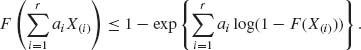
Let F be a log–convex distribution function. Then for any positive real numbers a1, …, ar,
(6.5.6) 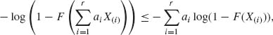
or equivalently
Let
(6.5.8) ![]()
Since F(X) ~ R(0, 1) and −log (1−R(0, 1)) ~ G(1, 1). The statistic G(X(i)) is distributed like the ith order statistic from a standard exponential distribution. Substitute in (6.5.7)
![]()
and
![]()
where Ai = ![]() ai, i = 1, …, r and X(0) ≡ 0. Moreover,
ai, i = 1, …, r and X(0) ≡ 0. Moreover,
(6.5.9) ![]()
Hence, if we define
![]()
then, from (6.5.7)
(6.5.10) 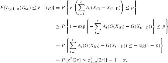
since 2 ![]() (n−i+1)(G(X(i)) − G(X(i−1))) ~ χ2[2r]. This result was published first by Barlow and Proschan (196).
(n−i+1)(G(X(i)) − G(X(i−1))) ~ χ2[2r]. This result was published first by Barlow and Proschan (196).
6.6 SIMULTANEOUS CONFIDENCE INTERVALS
It is often the case that we estimate simultaneously several parameters on the basis of the same sample values. One could determine for each parameter a confidence interval at level (1 − α) irrespectively of the confidence intervals of the other parameters. The result is that the overall confidence level is generally smaller than (1 − α). For example, suppose that (X1, …, Xn) is a sample of n i.i.d. random variables from N(μ, σ2). The sample mean ![]() and the sample variance S2 are independent statistics. Confidence intervals for μ and for σ, determined separately for each parameter, are
and the sample variance S2 are independent statistics. Confidence intervals for μ and for σ, determined separately for each parameter, are
![]()
and
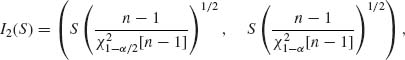
respectively. These intervals are not independent. We can state that the probability for μ to be in I1(![]() , S) is (1 − α) and that of σ to be in I2(S) is (1 − α). But, what is the probability that both statements are simultaneously true? According to the Bonferroni inequality (4.6.50)
, S) is (1 − α) and that of σ to be in I2(S) is (1 − α). But, what is the probability that both statements are simultaneously true? According to the Bonferroni inequality (4.6.50)
We see that a lower bound to the simultaneous coverage probability of (μ, σ) is according to (6.6.1), 1 − 2α. The actual simultaneous coverage probability of I1(![]() , S) and I2(S) can be determined by evaluating the integral
, S) and I2(S) can be determined by evaluating the integral
(6.6.2) ![]()
where gn(x) is the probability density function (p.d.f.) of χ2[n−1] and Φ(·) is the standard normal integral. The value of P(σ) is smaller than (1 − α). In order to make it at least (1 − α), we can modify the individual confidence probabilities of I1(![]() , S) and of I2(S) to be 1 − α /2. Then the simultaneous coverage probability will be between (1 − α) and (1 − α /2). This is a simple procedure that is somewhat conservative. It guarantees a simultaneous confidence level not smaller than the nominal (1 − α). This method of constructing simultaneous confidence intervals, called the Bonferroni method, has many applications. We have shown in Chapter 4 an application of this method in a two–way analysis of variance problem. Miller (196, p. 67) discussed an application of the Bonferroni method in a case of simultaneous estimation of k normal means.
, S) and of I2(S) to be 1 − α /2. Then the simultaneous coverage probability will be between (1 − α) and (1 − α /2). This is a simple procedure that is somewhat conservative. It guarantees a simultaneous confidence level not smaller than the nominal (1 − α). This method of constructing simultaneous confidence intervals, called the Bonferroni method, has many applications. We have shown in Chapter 4 an application of this method in a two–way analysis of variance problem. Miller (196, p. 67) discussed an application of the Bonferroni method in a case of simultaneous estimation of k normal means.
Consider again the linear model of full rank discussed in Section 5.3.2, in which the vector X has a multinormal distribution N(Aβ, σ2I). A is an n× p matrix of full rank and β is a p× 1 vector of unknown parameters. The least–squares estimator (LSE) of a specific linear combination of β, say λ = α′β, is ![]() = α′
= α′![]() = α′(A′A)−1A′X. We proved that
= α′(A′A)−1A′X. We proved that ![]() ∼ N(α′β, σ2α′(A′A)−1α). Moreover, an unbiased estimator of σ2 is
∼ N(α′β, σ2α′(A′A)−1α). Moreover, an unbiased estimator of σ2 is
![]()
where ![]() . Hence, a [1 − α] confidence interval for the particular parameter λ is
. Hence, a [1 − α] confidence interval for the particular parameter λ is
Suppose that we are interested in the simultaneous estimation of all (many) linear combinations belonging to a certain r–dimensional linear subspace 1 ≤ r ≤ p. For example, if we are interested in contrasts of the β–component, then λ = ![]() αiβi where Σ αi = 0. In this case, the linear subspace of all such contrasts is of dimension r = p−1. Let L be an r × p matrix with r row vectors that constitute a basis for the linear subspace under consideration. For example, in the case of all contrasts, the matrix L can be taken as the (p−1) × p matrix:
αiβi where Σ αi = 0. In this case, the linear subspace of all such contrasts is of dimension r = p−1. Let L be an r × p matrix with r row vectors that constitute a basis for the linear subspace under consideration. For example, in the case of all contrasts, the matrix L can be taken as the (p−1) × p matrix:
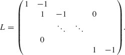
Every vector α belonging to the specified subspace is given by some linear combination α′ = γ′L. Thus, α′(A′A)−1α = γ′L(A′A)−1L′γ. Moreover,
(6.6.4) ![]()
and
(6.6.5) ![]()
where r is the rank of L. Accordingly,
(6.6.6) ![]()
and the probability is (1 − α) that β belongs to the ellipsoid
(6.6.7) ![]()
Eα (β, σ2, L) is a simultaneous confidence region for all α′β at level (1 − α). Consider any linear combination λ = α′β = γ′Lβ. The simultaneous confidence interval for λ can be obtained by the orthogonal projection of the ellipsoid Eα (β, ![]() 2, L) on the line l spanned by the vector γ. We obtain the following formula for the confidence limits of this interval
2, L) on the line l spanned by the vector γ. We obtain the following formula for the confidence limits of this interval
where λ= γ′L![]() = α′
= α′![]() . We see that in case of r = 1 formula (6.6.8) reduces to (6.6.3), otherwise the coefficient (rF1 − α[r, n−p])1/2 is greater than t1 − α /2[n−p]. This coefficient is called Scheffés S–coefficient. Various applications and modifications of the S–method have been proposed in the literature. For applications often used in statistical practice, see Miller (196, p. 54). Scheffé (1970) suggested some modifications for increasing the efficiency of the S–method for simultaneous confidence intervals.
. We see that in case of r = 1 formula (6.6.8) reduces to (6.6.3), otherwise the coefficient (rF1 − α[r, n−p])1/2 is greater than t1 − α /2[n−p]. This coefficient is called Scheffés S–coefficient. Various applications and modifications of the S–method have been proposed in the literature. For applications often used in statistical practice, see Miller (196, p. 54). Scheffé (1970) suggested some modifications for increasing the efficiency of the S–method for simultaneous confidence intervals.
6.7 TWO–STAGE AND SEQUENTIAL SAMPLING FOR FIXED WIDTH CONFIDENCE INTERVALS
We start the discussion with the problem of determining fixed–width confidence intervals for the mean μ of a normal distribution when the variance σ2 is unknown and can be arbitrarily large. We saw previously that if the sample consists of n i.i.d. random variables X1, …, Xn, where n is fixed before the sampling, then a UMAU confidence limit for μ are given, in correspondence to the t–test, by ![]() ± t1 − α /2[n−1]
± t1 − α /2[n−1] ![]() , where
, where ![]() and S are the sample mean and standard deviation, respectively. The width of this confidence interval is
and S are the sample mean and standard deviation, respectively. The width of this confidence interval is
(6.7.1) ![]()
Although the width of the interval is converging to zero, as n→ ∞, for each fixed n, it can be arbitrarily large with positive probability. The question is whether there exists another confidence interval with bounded width. We show now that there is no fixed–width confidence interval in the present normal case if the sample is of fixed size. Let Iδ (![]() , S) be any fixed width interval centered at
, S) be any fixed width interval centered at ![]() (
(![]() , S), i.e.,
, S), i.e.,
(6.7.2) ![]()
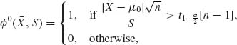
We show that the maximal possible confidence level is
This means that there is no statistic ![]() (
(![]() , S) for which Iδ (
, S) for which Iδ (![]() , S) is a confidence interval. Indeed,
, S) is a confidence interval. Indeed,
In Example 9.2, we show that ![]() (
(![]() , S) =
, S) = ![]() is a minimax estimator, which maximizes the minimum coverage. Accordingly,
is a minimax estimator, which maximizes the minimum coverage. Accordingly,
(6.7.5) ![]()
Substituting this result in (6.7.4), we readily obtain (6.7.3), by letting σ → ∞.
Stein’s two–stage procedure. Stein (1945) provided a two–stage solution to this problem of determining a fixed–width confidence interval for the mean μ. According to Stein’s procedure the sampling is performed in two stages:
Stage I:
(6.7.6) ![]()
where [x] designates the integer part of x.
![]()
Stage II:
The size of the second stage sample N2 = (N − n1)+ is a random variable, which is a function of the first stage sample variance ![]() . Since
. Since ![]() and
and ![]() are independent,
are independent, ![]() and N2 are independent. Moreover,
and N2 are independent. Moreover, ![]() N2 is conditionally independent of
N2 is conditionally independent of ![]() , given N2. Hence,
, given N2. Hence,
(6.7.7) 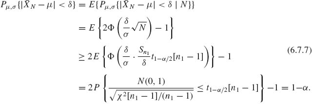
This proves that the fixed width interval Iδ (![]() N) based on the prescribed two–stage sampling procedure is a confidence interval. The Stein two–stage procedure is not an efficient one, unless one has good knowledge of how large n1 should be. If σ2 is known there exists a UMAU confidence interval of fixed size, i.e., Iδ (
N) based on the prescribed two–stage sampling procedure is a confidence interval. The Stein two–stage procedure is not an efficient one, unless one has good knowledge of how large n1 should be. If σ2 is known there exists a UMAU confidence interval of fixed size, i.e., Iδ (![]() n0(δ)) where
n0(δ)) where
(6.7.8) 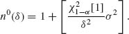
If n1 is close to n0(δ) the procedure is expected to be efficient. n0(δ) is, however, unknown. Various approaches have been suggested to obtain efficient procedures of sampling. We discuss here a sequential procedure that is asymptotically efficient. Note that the optimal sample size n0(δ) increases to infinity like 1/δ2 as δ → 0. Accordingly, a sampling procedure, with possibly random sample size, N, which yields a fixed–width confidence interval Iδ (![]() N) is called asymptotically efficient if
N) is called asymptotically efficient if
Sequential fixed–width interval estimation. Let {an} be a sequence of positive numbers such that an → ![]() [1] as n → ∞. We can set, for example, an = F1 − α [1, n] for all n ≥ n1 and an = ∞ for n < n1. Consider now the following sequential procedure:
[1] as n → ∞. We can set, for example, an = F1 − α [1, n] for all n ≥ n1 and an = ∞ for n < n1. Consider now the following sequential procedure:
(6.7.10) ![]()
According to the specified procedure, the sample size at termination is N(δ). N(δ) is called a stopping variable. We have to show first that N(δ) is finite with probability one, i.e.,
for each δ > 0. Indeed, for any given n,
(6.7.12) 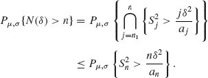
But
(6.7.13) ![]()
![]() as n→ ∞, therefore
as n→ ∞, therefore
(6.7.14) 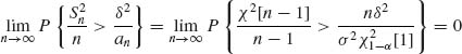
as n→ ∞. Thus, (6.7.11) is satisfied and N(δ) is a finite random variable. The present sequential procedure attains in large samples the required confidence level and is also an efficient one. One can prove in addition the following optimal properties:
(6.7.15) ![]()
This obviously implies the asymptotic efficiency (6.7.9). It is, however, a much stronger property. One does not have to pay, on the average, more than the equivalent of n1 + 1 observations. The question is whether we do not tend to stop too soon and thus lose confidence probability. Simons (1968) proved that if we follow the above procedure, n1 ≥ 3 and an = a for all n ≥ 3, then there exists a finite integer k such that
(6.7.16) ![]()
for all μ, σ and δ. This means that the possible loss of confidence probability is not more than the one associated with a finite number of observations. In other words, if the sample is large we generally attain the required confidence level.
We have not provided here proofs of these interesting results. The reader is referred to Zacks (1971, p. 560). The results were also extended to general classes of distributions originally by Chow and Robbins (1965), followed by studies of Starr (196), Khan (1969), Srivastava (1971), Ghosh, Mukhopadhyay, and Sen (1997), and Mukhopadhyay and de Silva (2009).
PART II: EXAMPLES
Example 6.1. It is assumed that the compressive strength of concrete cubes follows a log–normal distribution, LN(μ, σ2), with unknown parameters (μ, σ). It is desired that in a given production process the compressive strength, X, will not be smaller than ξ0 in (1 − β)× 100% of the concrete cubes. In other words, the β–quantile of the parent log–normal distribution should not be smaller than ξ0, where the β–quantile of LN(μ, σ2) is xβ = exp {μ + zβ σ}, and zβ is the β–quantile of N(0, 1). We observe a sample of n i.i.d. random variables X1, …, Xn and should decide on the basis of the observed sample values whether the strength requirement is satisfied. Let Yi = log Xi (i = 1, …, n). The sample mean and variance (![]() n,
n, ![]() ), where
), where ![]() , constitute a minimal sufficient statistic. On the basis of (
, constitute a minimal sufficient statistic. On the basis of (![]() n,
n, ![]() ), we wish to determine a (1 − α)–lower confidence limit, xα, β to the unknown β–quantile xβ. Accordingly, xα, β should satisfy the relationship
), we wish to determine a (1 − α)–lower confidence limit, xα, β to the unknown β–quantile xβ. Accordingly, xα, β should satisfy the relationship
![]()
xα, β is called a lower (1 − α, 1−β) guaranteed coverage tolerance limit. If xα, β ≥ ξ0, we say that the production process is satisfactory (meets the specified standard). Note that the problem of determining xα, β is equivalent to the problem of determining a (1 − α)–lower confidence limit to μ + zβ σ. This lower confidence limit is constructed in the following manner. We note first that if U ~ N(0, 1), then
![]()
where t[ν; δ] is the noncentral t–distribution. Thus, a (1 − α)–lower confidence limit for μ + zβ σ is
![]()
and xα, β = exp {ηα, β} is a lower (1 − α, 1 − β)–tolerance limit. ![]()
Example 6.2. Let X1, …, Xn be i.i.d. random variables representing the life length of electronic systems and distributed like ![]() . We construct two different (1 − α)–lower confidence limits for θ.
. We construct two different (1 − α)–lower confidence limits for θ.
(i) The minimal sufficient statistic is Tn = ΣXi. This statistic is distributed like ![]() χ2[2n]. Thus, for testing H0: θ ≤ θ0 against H1:θ > θ0 at level of significance α, the acceptance regions are of the form
χ2[2n]. Thus, for testing H0: θ ≤ θ0 against H1:θ > θ0 at level of significance α, the acceptance regions are of the form
![]()
The corresponding confidence intervals are
The lower confidence limit for θ is, accordingly,
![]()
(ii) Let ![]() . X(1) is distributed like
. X(1) is distributed like ![]() χ2[2]. Hence, the hypotheses H0: θ ≤ θ0 against H1: θ > θ0 can be tested at level α by the acceptance regions
χ2[2]. Hence, the hypotheses H0: θ ≤ θ0 against H1: θ > θ0 can be tested at level α by the acceptance regions
![]()
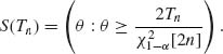
These regions yield the confidence intervals
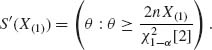
The corresponding lower confidence limit is ![]() [2]. Both families of confidence intervals provide lower confidence limits for the mean–time between failures, θ, at the same confidence level 1 − α. The question is which family is more efficient. Note that θα is a function of the minimal sufficient statistic, while θ′α is not. The expected value of θα is
[2]. Both families of confidence intervals provide lower confidence limits for the mean–time between failures, θ, at the same confidence level 1 − α. The question is which family is more efficient. Note that θα is a function of the minimal sufficient statistic, while θ′α is not. The expected value of θα is ![]() . This expected value is approximately, as n→ ∞,
. This expected value is approximately, as n→ ∞,
![]()
Thus, E{θα } is always smaller than θ, and approaches θ as n grows. On the other hand, the expected value of θ′α is
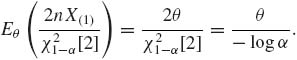
This expectation is about θ/3 when α = 0.05 and θ/4.6 when α = 0.01. It does not converge to θ as n increases. Thus, θ′α is an inefficient lower confidence limit of θ. ![]()
Example 6.3.
![]()
Accordingly, the UMA (1 − α)–lower confidence limit ![]() is
is
![]()
![]()
provided 1 ≤ X ≤ n−1. If X = 0, the lower confidence limit is θα (0) = 0. When X = n the lower confidence limit is θα (n) = α1/n. By employing the relationship between the central F–distribution and the beta distribution (see Section 2.14), we obtain the following for X ≥ 1 and R = 1:
![]()
If X ≥ 1 and R = 0 the lower limit, θ′α is obtained from (6.3.11) by substituting (X−1) for X. Generally, the lower limit can be obtained as the average Rθα + (1−R)θ′α. In practice, the nonrandomized solution (6.3.11) is often applied. ![]()
Example 6.4. Let X and Y be independent random variables having the normal distribution N(0, σ2) and N(0, ρσ2), respectively. We can readily prove that
![]()
where J has the negative binomial distribution ![]() . P(j; λ) designates the c.d.f. of the Poisson distributions with mean λ.
. P(j; λ) designates the c.d.f. of the Poisson distributions with mean λ. ![]() (σ2, ρ) is the coverage probability of a circle of radius one. We wish to determine a (1 − α)–lower confidence limit for
(σ2, ρ) is the coverage probability of a circle of radius one. We wish to determine a (1 − α)–lower confidence limit for ![]() (σ2, ρ), on the basis of n independent vectors, (X1, Y1), …, (Xn, Yn), when ρ is known. The minimal sufficient statistic is
(σ2, ρ), on the basis of n independent vectors, (X1, Y1), …, (Xn, Yn), when ρ is known. The minimal sufficient statistic is ![]() . This statistic is distributed like σ2χ2[2n]. Thus, the UMA (1 − α)–upper confidence limit for σ2
. This statistic is distributed like σ2χ2[2n]. Thus, the UMA (1 − α)–upper confidence limit for σ2
![]()
The Poisson family is an MLR one. Hence, by Karlin’s Lemma, the c.d.f. P(j; 1/2σ2) is an increasing function of σ2 for each j = 0, 1, …. Accordingly, if ![]() then P(j; 1/2σ2) ≤ P(j; 1/2
then P(j; 1/2σ2) ≤ P(j; 1/2![]() ). It follows that E
). It follows that E![]() . From this relationship we infer that
. From this relationship we infer that
![]()
is a (1 − α)–lower confidence limit for ![]() (σ2, ρ). We show now that
(σ2, ρ). We show now that ![]() (
(![]() , ρ) is a UMA lower confidence limit. By negation, if
, ρ) is a UMA lower confidence limit. By negation, if ![]() (
(![]() , ρ) is not a UMA, there exists another (1 − α) lower confidence limit,
, ρ) is not a UMA, there exists another (1 − α) lower confidence limit, ![]() say, and some 0 <
say, and some 0 < ![]() ′ <
′ < ![]() (σ2, ρ) such that
(σ2, ρ) such that
![]()
The function ![]() is a strictly increasing function of σ2. Hence, for each ρ there is a unique inverse
is a strictly increasing function of σ2. Hence, for each ρ there is a unique inverse ![]() (
(![]() ) for
) for ![]() (σ2, ρ). Thus, we obtain that
(σ2, ρ). Thus, we obtain that
![]()
where ![]() (
(![]() ′) < σ2. Accordingly,
′) < σ2. Accordingly, ![]() (
(![]() ) is a (1 − α)–upper confidence limit for σ2. But then the above inequality contradicts the assumption that
) is a (1 − α)–upper confidence limit for σ2. But then the above inequality contradicts the assumption that ![]() is UMA.
is UMA. ![]()
Example 6.5. Let X1, …, Xn be i.i.d. random variables distributed like N(μ, σ2). The UMP–unbiased test of the hypotheses
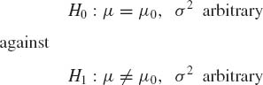
is the t–test
where ![]() and S are the sample mean and standard deviation, respectively. Correspondingly, the confidence interval
and S are the sample mean and standard deviation, respectively. Correspondingly, the confidence interval
![]()
is a UMAU at level (1 − α). ![]()
Example 6.6. In Example 4.11, we discussed the problem of comparing the binomial experiments in two clinics at which standard treatment is compared with a new (test) treatment. If Xij designates the number of successes in the jth sample at the ith clinic (i = 1, 2; j = 1, 2), we assumed that Xij are independent and Xij ~ B(n, θij). We consider the cross–product ratio
![]()
In Example 4.11, we developed the UMPU test of the hypothesis H0: ρ = 1 against H1: ρ ≠ 1. On the basis of this UMPU test, we can construct the UMAU confidence limits of ρ.
Let Y = X11, T1 = X11 + X12, T = X21 + X22, and S = X11 + X21. The conditional p.d.f. of Y given (T1, T2, S) under ρ was given in Example 4.11. Let H(y| T1, T2, S) denote the corresponding conditional c.d.f. This family of conditional distributions is MLR in Y. Thus, the quantiles of the distributions are increasing functions of ρ. Similarly, H(y| T1, T2, S) are strictly decreasing functions of ρ for each y = 0, 1, …, min (T1, S)> and each (T1, T2, S).
As shown earlier one–sided UMA confidence limits require in discrete cases further randomization. Thus, we have to draw at random two numbers R1 and R2 independently from a rectangular distribution R(0, 1) and solve simultaneously the equations
![]()
where ![]() 1 +
1 + ![]() 2 = α. Moreover, in order to obtain UMA unbiased intervals we have to determine ρ,
2 = α. Moreover, in order to obtain UMA unbiased intervals we have to determine ρ, ![]() ,
, ![]() 1 and
1 and ![]() 2 so that the two conditions of (4.4.2) will be satisfied simultaneously. One can write a computer algorithm to obtain this objective. However, the computations may be lengthy and tedious. If T1, T2 and S are not too small we can approximate the UMAU limits by the roots of the equations
2 so that the two conditions of (4.4.2) will be satisfied simultaneously. One can write a computer algorithm to obtain this objective. However, the computations may be lengthy and tedious. If T1, T2 and S are not too small we can approximate the UMAU limits by the roots of the equations
![]()
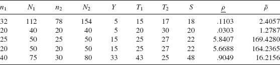
These equations have unique roots since the c.d.f. H(Y; T1, T2, S, ρ) is a strictly decreasing function of ρ for each (Y, T1, T2, S) having a continuous partial derivative with respect to ρ. The roots ρ and ![]() of the above equations are generally the ones used in applications. However, they are not UMAU. In Table 6.1, we present a few cases numerically. The confidence limits in Table 6.1 were computed by determining first the large sample approximate confidence limits (see Section 7.4) and then correcting the limits by employing the monotonicity of the conditional c.d.f. H(Y; T1, T2, S, ρ) in ρ. The limits are determined by a numerical search technique on a computer.
of the above equations are generally the ones used in applications. However, they are not UMAU. In Table 6.1, we present a few cases numerically. The confidence limits in Table 6.1 were computed by determining first the large sample approximate confidence limits (see Section 7.4) and then correcting the limits by employing the monotonicity of the conditional c.d.f. H(Y; T1, T2, S, ρ) in ρ. The limits are determined by a numerical search technique on a computer. ![]()
Table 6.1 0.95—Confidence Limits for the Cross–Product Ratio
Example 6.7. Let X1, X2, …, Xn be i.i.d. random variables having a negative–binomial distribution NB(![]() , ν); ν is known and 0 <
, ν); ν is known and 0 < ![]() < 1. A minimal sufficient statistic is Tn =
< 1. A minimal sufficient statistic is Tn = ![]() Xi, which has the negative–binomial distribution NB(
Xi, which has the negative–binomial distribution NB(![]() , nν). Consider the β–content one–sided prediction interval [0, G−1(β ;
, nν). Consider the β–content one–sided prediction interval [0, G−1(β ;![]() , ν)], where G−1(p;
, ν)], where G−1(p;![]() , ν) is the pth quantile of NB(
, ν) is the pth quantile of NB(![]() , ν). The c.d.f. of the negative–binomial distribution is related to the incomplete beta function ratio according to formula (2.2.12), i.e.,
, ν). The c.d.f. of the negative–binomial distribution is related to the incomplete beta function ratio according to formula (2.2.12), i.e.,
![]()
The pth quantile of the NB(![]() , ν) can thus be defined as
, ν) can thus be defined as
![]()
This function is nondecreasing in ![]() for each p and ν. Indeed,
for each p and ν. Indeed, ![]() = {NB(
= {NB(![]() , ν); 0 <
, ν); 0 < ![]() < 1} is an MLR family. Furthermore, since Tn ~ NB(
< 1} is an MLR family. Furthermore, since Tn ~ NB(![]() , nν), we can obtain a UMA upper confidence limit for
, nν), we can obtain a UMA upper confidence limit for ![]() ,
, ![]() α at confidence level γ = 1 − α. A nonrandomized upper confidence limit is the root
α at confidence level γ = 1 − α. A nonrandomized upper confidence limit is the root ![]() α of the equation
α of the equation
![]()
If we denote by β −1(p;a, b) the pth quantile of the beta distribution β (a, b) then ![]() α is given accordingly by
α is given accordingly by
![]()
The p–content (1 − α)–level tolerance interval is, therefore, [0, G−1(p;![]() α, ν)].
α, ν)]. ![]()
Example 6.8. In statistical life testing families of increasing failure rate (IFR) are often considered. The hazard or failure rate function h(x) corresponding to an absolutely continuous distribution F(x) is defined as
![]()
where f(x) is the p.d.f. A distribution function F(x) is IFR if h(x) is a nondecreasing function of x. The function F(x) is differentiable almost everywhere. Hence, the failure rate function h(x) can be written (for almost all x) as
![]()
Thus, if F(x) is an IFR distribution, −log (1−F(x)) is a convex function of x. A distribution function F(x) is called log–convex if its logarithm is a convex function of x. The tolerance limits that will be developed in the present example will be applicable for any log–convex distribution function.
Let X(1) ≤ ··· ≤ X(n) be the order statistic. It is instructive to derive first a (p, 1 − α)–lower tolerance limit for the simple case of the exponential distribution ![]() , 0 < θ < ∞. The pth quantile of
, 0 < θ < ∞. The pth quantile of ![]() is
is
![]()
Let Tn, r = ![]() (n−i + 1)(X(i) − X(i−1)) be the total life until the rth failure. Tn, r is distributed like
(n−i + 1)(X(i) − X(i−1)) be the total life until the rth failure. Tn, r is distributed like ![]() χ2[2r]. Hence, the UMA–(1 − α)–lower confidence limit for θ is
χ2[2r]. Hence, the UMA–(1 − α)–lower confidence limit for θ is
![]()
The corresponding (p, 1 − α) lower tolerance limit is
![]()
![]()
Example 6.9. The MLE of σ in samples from normal distributions is asymptotically normal with mean σ and variance σ2/2n. Therefore, in large samples,
![]()
for all μ, σ. The region given by
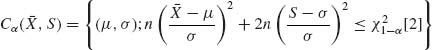
is a simultaneous confidence region with coverage probability approximately (1 − α). The points in the region Cα (![]() , S) satisfy the inequality
, S) satisfy the inequality
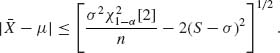
Hence, the values of σ in the region are only those for which the square root on the RHS of the above is real. Or, for all n > ![]() [2]/2,
[2]/2,
Note that this interval is not symmetric around S. Let σn and ![]() n denote the lower and upper limits of the σ interval. For each σ within this interval we determine a μ interval symmetrically around
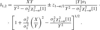
n denote the lower and upper limits of the σ interval. For each σ within this interval we determine a μ interval symmetrically around ![]() , as specified above. Consider the linear combination λ = a1μ + a2σ, where a1 + a2 = 1. We can obtain a (1 − α)–level confidence interval for λ from the region Cα (
, as specified above. Consider the linear combination λ = a1μ + a2σ, where a1 + a2 = 1. We can obtain a (1 − α)–level confidence interval for λ from the region Cα (![]() , S) by determining two lines parallel to a1μ + a2σ = 0 and tangential to the confidence region Cα (
, S) by determining two lines parallel to a1μ + a2σ = 0 and tangential to the confidence region Cα (![]() , S). These lines are given by the formula a1μ + a2σ = λα and a1μ = a2σ =
, S). These lines are given by the formula a1μ + a2σ = λα and a1μ = a2σ = ![]() α. The confidence interval is (λα,
α. The confidence interval is (λα, ![]() α). This interval can be obtained geometrically by projecting Cα (
α). This interval can be obtained geometrically by projecting Cα (![]() , S) onto the line l spanned by (a1, a2)); i.e., l = {(ρ a1, ρ a2); −∞ < ρ < ∞ }.
, S) onto the line l spanned by (a1, a2)); i.e., l = {(ρ a1, ρ a2); −∞ < ρ < ∞ }. ![]()
PART III: PROBLEMS
Section 6.2
6.2.1 Let X1, …, Xn be i.i.d. random variables having a common exponential distribution, G(![]() , 1), 0 < θ < ∞. Determine a (1 − α)–upper confidence limit for δ = e−θ.
, 1), 0 < θ < ∞. Determine a (1 − α)–upper confidence limit for δ = e−θ.
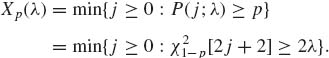
6.2.2 Let X1, …, Xn be i.i.d. random variables having a common Poisson distribution P(λ), 0 < λ < ∞. Determine a two–sided confidence interval for λ, at level 1 − α. [Hint: Let Tn = Σ Xi. Apply the relationship Pλ {Tn ≤ t} = P{χ2[2t + 2] ≥ 2nλ }, t = 0, 1, … to show that (λα, ![]() α) is a (1 − α)–level confidence interval, where
α) is a (1 − α)–level confidence interval, where ![]() and
and ![]() α =
α = ![]() .
.
6.2.3 Let X1, …, Xn be i.i.d. random variables distributed like G(λ, 1), 0 < λ < ∞; and let Y1, …, Ym be i.i.d. random variables distributed like G(η, 1), 0 < η < ∞. The X–variables and the Y–variables are independent. Determine a (1 − α)–upper confidence limit for ω = (1 + η /λ)−1 based on the statistic  .
.
6.2.4 Consider a vector X of n equicorrelated normal random variables, having zero mean, μ = 0, and variance σ2 [Problem 1, Section 5.3]; i.e., X ~ N(0, ![]() , ), where
, ), where ![]() , = σ2(1 − ρ)I +
, = σ2(1 − ρ)I + ![]() J; 0 < σ2 < ∞,
J; 0 < σ2 < ∞, ![]() < ρ < 1. Construct a (1 − α)–level confidence interval for ρ. [Hint:
< ρ < 1. Construct a (1 − α)–level confidence interval for ρ. [Hint:
6.2.5 Consider the linear regression model
![]()
where e1, …, en are i.i.d. N(0, σ2), x1, …, xn specified constants such that Σ(xi − ![]() )2 > 0. Determine the formulas of (1− α)–level confidence limits for β0, β1, and σ2. To what tests of significance do these confidence intervals correspond?
)2 > 0. Determine the formulas of (1− α)–level confidence limits for β0, β1, and σ2. To what tests of significance do these confidence intervals correspond?
6.2.6 Let X and Y be independent, normally distributed random variables, X ~ N(ξ, σ![]() ) and Y ~ N(η,
) and Y ~ N(η, ![]() ); −∞ < ξ < ∞, 0 < η < ∞, σ1 and σ2 known. Let δ = ξ /η. Construct a (1 − α)–level confidence interval for δ.
); −∞ < ξ < ∞, 0 < η < ∞, σ1 and σ2 known. Let δ = ξ /η. Construct a (1 − α)–level confidence interval for δ.
Section 6.3
6.3.1 Prove that if an upper (lower) confidence limit for a real parameter θ is based on a UMP test of H0: θ ≥ θ0 (θ ≤ θ0) against H1: θ < θ0 (θ > θ0) then the confidence limit is UMA.
6.3.2 Let X1, …, Xn be i.i.d. having a common two parameter exponential distribution, i.e., X ~ μ + G(![]() , 1); −∞ < μ < ∞, 0 < β < ∞.
, 1); −∞ < μ < ∞, 0 < β < ∞.
[Hint: See Problem 1, Section 4.5.]
6.3.3 Let X1, …, Xn be i.i.d. random variables having a common rectangular distribution R(0, θ); 0 < θ < ∞. Determine the (1 − α)–level UMA lower confidence limit for θ.
6.3.4 Consider the random effect model, Model II, of ANOVA (Example 3.9). Derive the (1 − α)–level confidence limits for σ2 and τ2. Does this system of confidence intervals have optimal properties?
Section 6.4
6.4.1 Let X1, …, Xn be i.i.d. random variables having a Poisson distribution P(λ), 0 < λ < ∞. Determine a (p, 1 − α) guaranteed coverage upper tolerance limit for X.
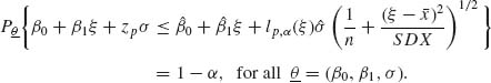
6.4.2 Consider the normal simple regression model (Problem 7, Section 5.4). Let ξ be a point in the range of controlled experimental levels x1, …, xn (regressors). A p–content prediction limit at ξ is the point ηp = β0 + β1 ξ + zpσ.
Section 6.5
6.5.1 Consider a symmetric continuous distribution F(x − μ), −∞ < μ < ∞. How large should the sample size n be so that (X(i), X(n−i+1)) is a distribution–free confidence interval for μ, at level 1 − α = 0.95, when
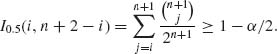
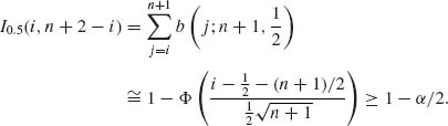
6.5.2 Apply the large sample normal approximation to the binomial distribution to show that for large size random samples from symmetric distribution the (1 − α)–level distribution free confidence interval for the median is given by (X(i), X(n−i+1)), where ![]() (David, 1970, p. 14).
(David, 1970, p. 14).
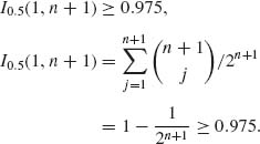
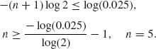
6.5.3 How large should the sample size n be so that a (p, γ) upper tolerance limit will exist with p = 0.95 and γ = 0.95?
6.5.4 Let F(x) be a continuous c.d.f. and X(1) ≤ ··· ≤ X(n) the order statistic of a random sample from such a distribution. Let F−1(p) and F−1(q), with 0 < p < q < 1, be the pth and qth quantiles of this distribution. Consider the interval Ep, q = (F−1(p), F−1(q)). Let p ≤ r < s ≤ n. Show that
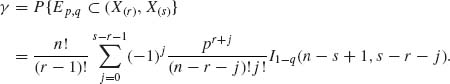
If q = 1 − β /2 and p = β /2 then (X(r), X(s)) is a (1 − β, γ) tolerance interval, where γ is given by the above formula.
Section 6.6
6.6.1 In a one–way ANOVA k = 10 samples were compared. Each of the samples consisted of n = 10 observations. The sample means in order of magnitude were: 15.5, 17.5, 20.2, 23.3, 24.1, 25.5, 28.8, 28.9, 30.1, 30.5. The pooled variance estimate is ![]() = 105.5. Perform the Scheffé simultaneous testing to determine which differences are significant at level α = 0.05.
= 105.5. Perform the Scheffé simultaneous testing to determine which differences are significant at level α = 0.05.
6.6.2 n = 10 observations Yij (i = 1, …, 3; j = 1, …, n) were performed at three values of x. The sample statistics are:
![]()
Section 6.7
6.7.1 Let X1, X2, … be a sequence of i.i.d. random variables having a common log–normal distribution, LN(μ, σ2). Consider the problem of estimating ξ = exp {μ + σ2/2}. The proportional–closeness of an estimator, ![]() , is defined as Pθ {|
, is defined as Pθ {|![]() −ξ| < λ ξ }, where λ is a specified positive real.
−ξ| < λ ξ }, where λ is a specified positive real.
6.7.2 Show that if ![]() is a family of distribution function depending on a location parameter of the translation type, i.e., F(x;θ) = F0(x − θ), −∞ < θ < ∞, then there exists a fixed width confidence interval estimator for θ.
is a family of distribution function depending on a location parameter of the translation type, i.e., F(x;θ) = F0(x − θ), −∞ < θ < ∞, then there exists a fixed width confidence interval estimator for θ.
6.7.3 Let X1, …, Xn be i.i.d. having a rectangular distribution R(0, θ), 0 < θ < 2. Let X(n) be the sample maximum, and consider the fixed–width interval estimator Iδ (X(n)) = (X(n), X(n) + δ), 0 < δ < 1. How large should n be so that Pθ {θ ![]() Iδ (X(n))} ≥ 1 − α, for all θ ≤ 2?
Iδ (X(n))} ≥ 1 − α, for all θ ≤ 2?
6.7.4 Consider the following three–stage sampling procedure for estimating the mean of a normal distribution. Specify a value of δ, 0 < δ < ∞.
![]()
![]()
independent observations. Let N = n1 + N2 + N3. Let ![]() N be the average of the sample of size N and Iδ (
N be the average of the sample of size N and Iδ (![]() n) = (
n) = (![]() N − δ,
N − δ, ![]() N + δ).
N + δ).
PART IV: SOLUTION TO SELECTED PROBLEMS
6.2.2 X1, …, Xn are i.i.d. P(λ). Tn = ![]() Xi ∼ P(nλ)
Xi ∼ P(nλ)
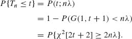
The UMP test of H0: λ ≥ λ0 against H1:λ < λ0 is ![]() (Tn) = I(Tn < tα). Note that P(χ2[2tα + 2] ≥ 2nλ0) = α if 2nλ0 =
(Tn) = I(Tn < tα). Note that P(χ2[2tα + 2] ≥ 2nλ0) = α if 2nλ0 = ![]() [2tα + 2]. For two–sided confidence limits, we have λα =
[2tα + 2]. For two–sided confidence limits, we have λα = ![]() and
and ![]() α =
α = ![]() .
.
6.2.4 Without loss of generality assume that σ2 = 1
![]()
where ![]() < 1, n is the dimension of X, and J = 1n1′n.
< 1, n is the dimension of X, and J = 1n1′n.
![]()
Note that H((1 − ρ)I + ρ J)H′ = diag ((1−ρ) + nρ, (1 − ρ), …, (1 − ρ)).
Hence, for a given 0 < α < 1,
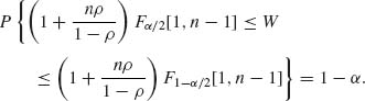
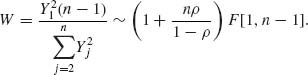
Recall that Fα /2[1, n − 1] = ![]() . Let
. Let
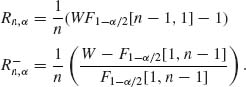
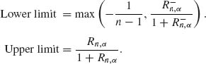
Since ρ /(1 − ρ) is a strictly increasing function of ρ, the confidence limits for ρ are
6.2.6 The method used here is known as Fieller’s method. Let U = X − δY. Accordingly, U ∼ N(0, σ ![]() + δ2
+ δ2![]() ) and
) and
![]()
It follows that there are two real roots (if they exist) of the quadratic equation in δ,
![]()
These roots are given by
It follows that if ![]() [1] the two real roots exist. These are the confidence limits for δ.
[1] the two real roots exist. These are the confidence limits for δ.
6.4.1 The m.s.s. for λ is Tn = ![]() Xi. A p–quantile of
Xi. A p–quantile of ![]() (λ) is
(λ) is
Since ![]() (λ) is an MLR family in X, the (p, 1 − α) guaranteed upper tolerance limit is
(λ) is an MLR family in X, the (p, 1 − α) guaranteed upper tolerance limit is
![]()
where ![]() α (Tn) =
α (Tn) = ![]()
![]() [2Tn+2] is the upper confidence limit for λ. Accordingly,
[2Tn+2] is the upper confidence limit for λ. Accordingly,
![]()
6.5.1 (i) Since F is symmetric, if i = 1, then j = n. Thus,
Or,
For n = 8, ![]() = 0.0195. For n = 7,
= 0.0195. For n = 7, ![]() = 0.0352. Thus, n =8.
= 0.0352. Thus, n =8.
Or
![]()
For n = 10, we get ![]() = 0.0327. For n = 11, we get
= 0.0327. For n = 11, we get ![]() = 0.0193. Thus, n = 11.
= 0.0193. Thus, n = 11.
6.5.2
For large n, by Central Limit Theorem,
Thus,
6.7.1 Let Yi = log Xi, i = 1, 2, …. If we have a random sample of fixed size n, then the MLE of ξ is ![]() n = exp
n = exp ![]() , where
, where ![]() n =
n = ![]()
![]() Yi and
Yi and ![]() 2 =
2 = ![]()
![]() (Yi −
(Yi − ![]() n)2.
n)2.
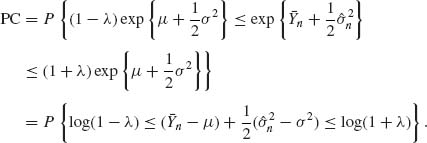
For large values of n, the distribution of![]() is approximately, by CLT,
is approximately, by CLT, ![]() .
.
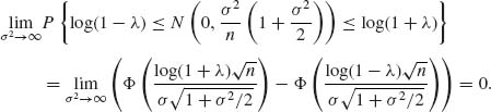
Hence, there exists no fixed sample procedure with PC ≥ γ > 0.
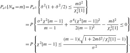
![]()
Accordingly, we define the stopping variable
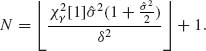
If {N ≤ m} stop sampling and use ![]() . On the other hand, if {N > m} go to Stage II.
. On the other hand, if {N > m} go to Stage II.
For l = m + 1, m + 2, … let
then
![]()