CHAPTER 5
Statistical Estimation
PART I: THEORY
5.1 GENERAL DISCUSSION
Point estimators are sample statistics that are designed to yield numerical estimates of certain characteristics of interest of the parent distribution. While in testing hypotheses we are generally interested in drawing general conclusions about the characteristics of the distribution, for example, whether its expected value (mean) is positive or negative, in problems of estimation we are concerned with the actual value of the characteristic. Generally, we can formulate, as in testing of hypotheses, a statistical model that expresses the available information concerning the type of distribution under consideration. In this connection, we distinguish between parametric and nonparametric (or distribution free) models. Parametric models specify parametric families of distributions. It is assumed in these cases that the observations in the sample are generated from a parent distribution that belongs to the prescribed family. The estimators that are applied in parametric models depend in their structure and properties on the specific parametric family under consideration. On the other hand, if we do not wish, for various reasons, to subject the estimation procedure to strong assumptions concerning the family to which the parent distribution belongs, a distribution free procedure may be more reasonable. In Example 5.1, we illustrate some of these ideas.
This chapter is devoted to the theory and applications of these types of estimators: unbiased, maximum likelihood, equivariant, moment equations, pretest, and robust estimators.
5.2 UNBIASED ESTIMATORS
5.2.1 General Definition and Example
Unbiased estimators of a characteristic θ(F) of F in ![]() is an estimator
is an estimator ![]() (X) satisfying
(X) satisfying
(5.2.1) ![]()
where X is a random vector representing the sample random variables. For example, if θ (F) = EF{X}, assuming that EF{|X|} < ∞ for all F ![]()
![]() , then the sample mean
, then the sample mean ![]() is an unbiased estimator of θ(F). Moreover, if VF{X} < ∞ for all F
is an unbiased estimator of θ(F). Moreover, if VF{X} < ∞ for all F ![]()
![]() then the sample variance
then the sample variance ![]() is an unbiased estimator of VF{X}. We note that all the examples of unbiased estimators given here are distribution free. They are valid for any distribution for which the expectation or the variance exist. For parametric models one can do better by using unbiased estimators which are functions of the minimal sufficient statistics. The comparison of unbiased estimators is in terms of their variances. Of two unbiased estimators, the one having a smaller variance is considered better, or more efficient. One reason for preferring the unbiased estimator with the smaller variance is in the connection between the variance of the estimator and the probability that it belongs to a fixed–width interval centered at the unknown characteristic. In Example 5.2, we illustrate a case in which the distribution–free estimator of the expectation is inefficient.
is an unbiased estimator of VF{X}. We note that all the examples of unbiased estimators given here are distribution free. They are valid for any distribution for which the expectation or the variance exist. For parametric models one can do better by using unbiased estimators which are functions of the minimal sufficient statistics. The comparison of unbiased estimators is in terms of their variances. Of two unbiased estimators, the one having a smaller variance is considered better, or more efficient. One reason for preferring the unbiased estimator with the smaller variance is in the connection between the variance of the estimator and the probability that it belongs to a fixed–width interval centered at the unknown characteristic. In Example 5.2, we illustrate a case in which the distribution–free estimator of the expectation is inefficient.
5.2.2 Minimum Variance Unbiased Estimators
In Example 5.2, one can see a case where an unbiased estimator, which is not a function of the minimal sufficient statistic (m.s.s.), has a larger variance than the one based on the m.s.s. The question is whether this result holds generally. The main theorem of this section establishes that if a family of distribution functions admits a complete sufficient statistic then the minimum variance unbiased estimator (MVUE) is unique, with probability one, and is a function of that statistic. The following is the fundamental theorem of the theory of unbiased estimation. It was proven by Rao (1945, 1947, 1949), Blackwell (1947), and Lehmann and Scheffé (1950).
Theorem 5.2.1 (The Rao–Blackwell–Lehmann–Scheffé Theorem) Let ![]() = {F(x;θ);θ
= {F(x;θ);θ ![]() Θ} be a parametric family of distributions of a random vector X = (X1, …, Xn). Suppose that ω = g(θ) has an unbiased estimator
Θ} be a parametric family of distributions of a random vector X = (X1, …, Xn). Suppose that ω = g(θ) has an unbiased estimator ![]() (X). If
(X). If ![]() admits a (minimal) sufficient statistic T(X) then
admits a (minimal) sufficient statistic T(X) then
(5.2.2) ![]()
is an unbiased estimator of ω and
for all θ ![]() Θ. Furthermore, if T(X) is a complete sufficient statistic then
Θ. Furthermore, if T(X) is a complete sufficient statistic then ![]() is essentially the unique minimum variance, unbiased (MVU) estimator, for each θ in Θ.
is essentially the unique minimum variance, unbiased (MVU) estimator, for each θ in Θ.
Proof. (i) Since T(X) is a sufficient statistic, the conditional expectation E{![]() (X)| T(X)} does not depend on θ and is therefore a statistic. Moreover, according to the law of the iterated expectations and since
(X)| T(X)} does not depend on θ and is therefore a statistic. Moreover, according to the law of the iterated expectations and since ![]() (X) is unbiased, we obtain
(X) is unbiased, we obtain
(5.2.4) 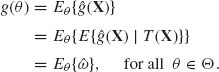
Hence, ![]() is an unbiased estimator of g(θ). By the law of the total variance,
is an unbiased estimator of g(θ). By the law of the total variance,
The second term on the RHS of (5.2.5) is the variance of ![]() . Moreover, Var{
. Moreover, Var{![]() (X)| T(X)} ≥ 0 with probability one for each θ in Θ. Hence, the first term on the RHS of (5.2.5) is nonnegative. This establishes (5.2.3).
(X)| T(X)} ≥ 0 with probability one for each θ in Θ. Hence, the first term on the RHS of (5.2.5) is nonnegative. This establishes (5.2.3).
(ii) Let T(X) be a complete sufficient statistic and assume that ![]() =
= ![]() 1(T(X)). Let
1(T(X)). Let ![]() (X) be any unbiased estimator of ω = g(θ), which depends on T(X), i.e.,
(X) be any unbiased estimator of ω = g(θ), which depends on T(X), i.e., ![]() (X) =
(X) = ![]() 2(T(X)). Then, Eθ {
2(T(X)). Then, Eθ {![]() } = Eθ {
} = Eθ {![]() (X)} for all θ. Or, equivalently
(X)} for all θ. Or, equivalently
(5.2.6) ![]()
Hence, from the completeness of T(X), ![]() 1(T) =
1(T) = ![]() 2(T) with probability one for each θ
2(T) with probability one for each θ ![]() Θ. This proves that
Θ. This proves that ![]() =
= ![]() 1(T) is essentially unique and implies also that
1(T) is essentially unique and implies also that ![]() has the minimal variance at each θ. QED
has the minimal variance at each θ. QED
Part (i) of the above theorem provides also a method of constructing MVUEs. One starts with any unbiased estimator, as simple as possible, and then determines its conditional expectation, given T(X). This procedure of deriving MVUEs is called in the literature “Rao–Blackwellization.” Example 5.3 illustrates this method.
In the following section, we prove and illustrate an information lower bound for variances of unbiased estimators. This lower bound plays an important role in the theory of statistical inference.
5.2.3 The Cramér–Rao Lower Bound for the One–Parameter Case
The following theorem was first proven by Fréchet (1943) and then by Rao (1945) and Cramér (1946). Although conditions (i)–(iii), (v) of the following theorem coincide with conditions (3.7.8) we restate them. Conditions (i)–(iv) will be labeled the Cramér–Rao (CR) regularity conditions.
Theorem 5.2.2. Let ![]() be a one–parameter family of distributions of a random vector X = (X1, …, Xn), having probability density functions (p.d.f.s) f(x;θ), θ
be a one–parameter family of distributions of a random vector X = (X1, …, Xn), having probability density functions (p.d.f.s) f(x;θ), θ ![]() Θ. Let ω (θ) be a differentiable function of θ and
Θ. Let ω (θ) be a differentiable function of θ and ![]() (X) an unbiased estimator of ω (θ). Assume that the following regularity conditions hold:
(X) an unbiased estimator of ω (θ). Assume that the following regularity conditions hold:
![]()
![]()
 .
.
Proof. Consider the covariance, for a given θ value, between ![]() log f(X;θ) and
log f(X;θ) and ![]() (X). We have shown in (3.7.3) that under the above regularity conditions Eθ
(X). We have shown in (3.7.3) that under the above regularity conditions Eθ ![]() . Hence,
. Hence,
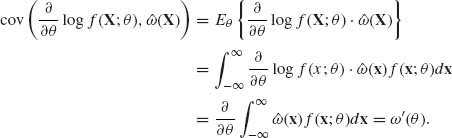
The interchange of differentiation and integration is justified by condition (iv). On the other hand, by the Schwarz inequality
since the variance of ![]() is equal to the Fisher information function In(θ), and the square of the coefficient of correlation between
is equal to the Fisher information function In(θ), and the square of the coefficient of correlation between ![]() (X) and
(X) and ![]() cannot exceed 1. From (5.2.8) and (5.2.9), we obtain the Cramér – Rao inequality (5.2.7). QED
cannot exceed 1. From (5.2.8) and (5.2.9), we obtain the Cramér – Rao inequality (5.2.7). QED
We show that if an unbiased estimator ![]() (X) has a distribution of the one–parameter exponential type, then the variance of
(X) has a distribution of the one–parameter exponential type, then the variance of ![]() (X) attains the Cramér – Rao lower bound. Indeed, let
(X) attains the Cramér – Rao lower bound. Indeed, let
(5.2.10) ![]()
where ![]() (θ) and K(θ) are differentiable, and
(θ) and K(θ) are differentiable, and ![]() ′(θ) ≠ 0 for all θ then
′(θ) ≠ 0 for all θ then
(5.2.11) ![]()
and
(5.2.12) ![]()
Since ![]() (X) is a sufficient statistic, In(θ) is equal to
(X) is a sufficient statistic, In(θ) is equal to
(5.2.13) ![]()
Moreover, ![]() (X) is an unbiased estimator of g(θ) = +K′(θ)/
(X) is an unbiased estimator of g(θ) = +K′(θ)/![]() ′(θ). Hence, we readily obtain that
′(θ). Hence, we readily obtain that
(5.2.14) ![]()
We ask now the question: if the variance of an unbiased estimator ![]() (X) attains the Cramér – Rao lower bound, can we infer that its distribution is of the one–parameter exponential type? Joshi (1976) provided a counter example. However, under the right regularity conditions the above implication can be made. These conditions were given first by Wijsman (1973) and then generalized by Joshi (1976).
(X) attains the Cramér – Rao lower bound, can we infer that its distribution is of the one–parameter exponential type? Joshi (1976) provided a counter example. However, under the right regularity conditions the above implication can be made. These conditions were given first by Wijsman (1973) and then generalized by Joshi (1976).
Bhattacharyya (1946) generalized the Cramér – Rao lower bound to (regular) cases where ω (θ) is k–times differentiable at all θ. This generalization shows that, under further regularity conditions, if ωi(θ) is the ith derivative of ω(θ) and V is a k × k positive definite matrix, for all θ, with elements
![]()
then
Fend (1959) has proven that if the distribution of X belongs to the one–parameter exponential family, and if the variance of an unbiased estimator of ω(θ), ![]() (X), attains the kth order Bhattacharyya lower bound (BLB) for all θ, but does not attain the (k – 1)st lower bound, then
(X), attains the kth order Bhattacharyya lower bound (BLB) for all θ, but does not attain the (k – 1)st lower bound, then ![]() (X) is a polynomial of degree k in U(X).
(X) is a polynomial of degree k in U(X).
5.2.4 Extension of the Cramér – Rao Inequality to Multiparameter Cases
The Cramér – Rao inequality can be generalized to estimation problems in k–parameter models in the following manner. Suppose that ![]() is a family of distribution functions having density functions (or probability functions) f(x;θ) where θ = (θ1, …, θk)′ is a k–dimensional vector. Let I(θ) denote a k × k Fisher information matrix, with elements
is a family of distribution functions having density functions (or probability functions) f(x;θ) where θ = (θ1, …, θk)′ is a k–dimensional vector. Let I(θ) denote a k × k Fisher information matrix, with elements
![]()
i, j = 1, …, k. We obviously assume that for each θ in the parameter space Θ, Iij(θ) is finite. It is easy to show that the matrix I(θ) is nonnegative definite. We will assume, however, that the Fisher information matrix is positive definite. Furthermore, let g1(θ), …, gr(θ) be r parametric functions r = 1, 2, …, k. Define the matrix of partial derivatives
(5.2.16) ![]()
where Dij(θ) = ![]() . Let
. Let ![]() (X) be an r–dimensional vector of unbiased estimators of g1(θ), …, gr(θ), i.e.,
(X) be an r–dimensional vector of unbiased estimators of g1(θ), …, gr(θ), i.e., ![]() (X) = (
(X) = (![]() 1(X), …,
1(X), …, ![]() r(X)). Let
r(X)). Let ![]() (
(![]() ) denote the variance – covariance matrix of
) denote the variance – covariance matrix of ![]() (X). The Cramér – Rao inequality can then be generalized, under regularity conditions similar to those of the theorem, to yield the inequality
(X). The Cramér – Rao inequality can then be generalized, under regularity conditions similar to those of the theorem, to yield the inequality
(5.2.17) ![]()
in the sense that ![]() (
(![]() ) – D(θ)(I(θ))−1D′(θ) is a nonnegative definite matrix. In the special case of one parameter function g(θ), if
) – D(θ)(I(θ))−1D′(θ) is a nonnegative definite matrix. In the special case of one parameter function g(θ), if ![]() (X) is an unbiased estimator of g(θ) then
(X) is an unbiased estimator of g(θ) then
where ![]() g(θ) =
g(θ) = ![]() .
.
5.2.5 General Inequalities of the Cramér – Rao Type
The Cramér – Rao inequality is based on four stringent assumptions concerning the family of distributions under consideration. These assumptions may not be fulfilled in cases of practical interest. In order to overcome this difficulty, several studies were performed and various different general inequalities were suggested. Blyth and Roberts (1972) provided a general theoretical framework for these generalizations. We present here the essential results.
Let X1, …, Xn be independent and identically distributed (i.i.d.) random variables having a common distribution F that belongs to a one–parameter family ![]() , having p.d.f. f(x;θ), θ
, having p.d.f. f(x;θ), θ ![]() Θ. Suppose that g(θ) is a parametric function considered for estimation. Let T(X) be a sufficient statistic for
Θ. Suppose that g(θ) is a parametric function considered for estimation. Let T(X) be a sufficient statistic for ![]() and let
and let ![]() (T) be an unbiased estimator of g(θ). Let W(T;θ) be a real–valued random variable such that Varθ {W(T;θ)} > 0 and finite for every θ. We also assume that 0 < Varθ {
(T) be an unbiased estimator of g(θ). Let W(T;θ) be a real–valued random variable such that Varθ {W(T;θ)} > 0 and finite for every θ. We also assume that 0 < Varθ {![]() (T)} < ∞ for each θ in Θ. Then, from the Schwarz inequality, we obtain
(T)} < ∞ for each θ in Θ. Then, from the Schwarz inequality, we obtain
for every θ ![]() Θ. We recall that for the Cramér – Rao inequality, we have used
Θ. We recall that for the Cramér – Rao inequality, we have used
(5.2.20) ![]()
where h(t;θ) is the p.d.f. of T at θ.
Chapman and Robbins (1951) and Kiefer (1952) considered a family of random variables W![]() (T;θ), where
(T;θ), where ![]() ranges over Θ and is given by the likelihood ratio W
ranges over Θ and is given by the likelihood ratio W![]() (T;θ) =
(T;θ) = ![]() . The inequality (5.2.19) then becomes
. The inequality (5.2.19) then becomes
One obtains then that (5.2.21) holds for each ![]() in Θ. Hence, considering the supremum of the RHS of (5.2.21) over all values of
in Θ. Hence, considering the supremum of the RHS of (5.2.21) over all values of ![]() , we obtain
, we obtain
(5.2.22) ![]()
where A(θ, ![]() ) = Varθ {W
) = Varθ {W![]() (T;θ)}. Indeed,
(T;θ)}. Indeed,
(5.2.23) ![]()
This inequality requires that all the p.d.f.s of T, i.e., h(t;θ), θ ![]() Θ, will be positive on the same set, which is independent of any unknown parameter. Such a condition restricts the application of the Chapman – Robbins inequality. We cannot consider it, for example, in the case of a life–testing model in which the family
Θ, will be positive on the same set, which is independent of any unknown parameter. Such a condition restricts the application of the Chapman – Robbins inequality. We cannot consider it, for example, in the case of a life–testing model in which the family ![]() is that of location–parameter exponential distributions, i.e., f(x;θ) = I { x ≥ θ } exp{-(x – θ)}, with 0 < θ < ∞. However, one can consider the variable W
is that of location–parameter exponential distributions, i.e., f(x;θ) = I { x ≥ θ } exp{-(x – θ)}, with 0 < θ < ∞. However, one can consider the variable W![]() (T;θ) for all
(T;θ) for all ![]() values such that h(t;
values such that h(t;![]() ) = 0 on the set Nθ = {t: h(t;θ) = 0}. In the above location–parameter example, we can restrict attention to the set of
) = 0 on the set Nθ = {t: h(t;θ) = 0}. In the above location–parameter example, we can restrict attention to the set of ![]() values that are greater than Θ. If we denote this set by C(θ) then we have the Chapman – Robbins inequality as follow:
values that are greater than Θ. If we denote this set by C(θ) then we have the Chapman – Robbins inequality as follow:
(5.2.24) ![]()
The Chapman – Robbins inequality is applicable, as we have seen in the previous example, in cases where the Cramér – Rao inequality is inapplicable. On the other hand, we can apply the Chapman – Robbins inequality also in cases satisfying the Cramér – Rao regularity conditions. The question is then, what is the relationship between the Chapman – Robbins lower bound and Cramér – Rao lower bound. Chapman and Robbins (1951) have shown that their lower bound is greater than or equal to the Cramér – Rao lower bound for all θ.
5.3 THE EFFICIENCY OF UNBIASED ESTIMATORS IN REGULAR CASES
Let ![]() 1(X) and
1(X) and ![]() 2(X) be two unbiased estimators of g(θ). Assume that the density functions and the estimators satisfy the Cramér – Rao regularity conditions. The relative efficiency of
2(X) be two unbiased estimators of g(θ). Assume that the density functions and the estimators satisfy the Cramér – Rao regularity conditions. The relative efficiency of ![]() 1(X) to
1(X) to ![]() 2(X) is defined as the ratio of their variances,
2(X) is defined as the ratio of their variances,
where ![]() is the variance of
is the variance of ![]() i(X) at θ. In order to compare all the unbiased estimators of g(θ) on the same basis, we replace
i(X) at θ. In order to compare all the unbiased estimators of g(θ) on the same basis, we replace ![]() by the Cramér – Rao lower bound (5.2.7). In this manner, we obtain the efficiency function
by the Cramér – Rao lower bound (5.2.7). In this manner, we obtain the efficiency function
(5.3.2) ![]()
for all θ ![]() Θ. This function assumes values between zero and one. It is equal to one, for all θ, if and only if
Θ. This function assumes values between zero and one. It is equal to one, for all θ, if and only if ![]() attains the Cramér – Rao lower bound, or equivalently, if the distribution of
attains the Cramér – Rao lower bound, or equivalently, if the distribution of ![]() (X) is of the exponential type.
(X) is of the exponential type.
Consider the covariance between ![]() (X) and the score function S(X;θ) =
(X) and the score function S(X;θ) = ![]() log f(x;θ). As we have shown in the proof of the Cramér – Rao inequality that
log f(x;θ). As we have shown in the proof of the Cramér – Rao inequality that
where ρθ (![]() , S) is the coefficient of correlation between the estimator
, S) is the coefficient of correlation between the estimator ![]() and the score function, S(X;θ), at θ. Hence, the efficiency function is
and the score function, S(X;θ), at θ. Hence, the efficiency function is
(5.3.4) ![]()
Moreover, the relative efficiency of two unbiased estimators ![]() 1 and
1 and ![]() 2 is given by
2 is given by
(5.3.5) ![]()
This relative efficiency can be expressed also in terms of the ratio of the Fisher information functions obtained from the corresponding distributions of the estimators. That is, if h(![]() i;θ), i = 1, 2, is the p.d.f. of
i;θ), i = 1, 2, is the p.d.f. of ![]() i and I
i and I![]() i (θ) =
i (θ) = ![]() then
then
It is a straightforward matter to show that for every unbiased estimator ![]() of g(θ) and under the Cramér – Rao regularity conditions
of g(θ) and under the Cramér – Rao regularity conditions
Thus, the relative efficiency function (5.3.6) can be written, for cases satisfying the Cramér – Rao regularity condition, in the form
where ![]() 1(X) and
1(X) and ![]() 2(X) are unbiased estimators of g1(θ) and g2(θ), respectively. If the two estimators are unbiased estimators of the same function g(θ) then (5.3.8) is reduced to (5.3.1). The relative efficiency function (5.3.8) is known as the Pitman relative efficiency. It relates both the variances and the derivatives of the bias functions of the two estimators (see Pitman, 1948).
2(X) are unbiased estimators of g1(θ) and g2(θ), respectively. If the two estimators are unbiased estimators of the same function g(θ) then (5.3.8) is reduced to (5.3.1). The relative efficiency function (5.3.8) is known as the Pitman relative efficiency. It relates both the variances and the derivatives of the bias functions of the two estimators (see Pitman, 1948).
The information function of an estimator can be generalized to the multiparameter regular case (see Bhapkar, 1972). Let θ = (θ1, …, θk) be a vector of k–parameters and I(θ) be the Fisher information matrix (corresponding to one observation). If g1(θ), …, gr(θ), 1 ≤ r ≤ k, are functions satisfying the required differentiability conditions and ![]() 1(X), …,
1(X), …, ![]() r(X) are the corresponding unbiased estimators then, from (5.2.18),
r(X) are the corresponding unbiased estimators then, from (5.2.18),
(5.3.9) ![]()
where n is the sample size. Note that if r = k then D(θ) is nonsingular (the parametric functions g1(θ), …, gk(θ) are linearly independent), and we can express the above inequality in the form
(5.3.10) ![]()
Accordingly, and in analogy to (5.3.7), we define the amount of information in the vector estimator ![]() as
as
(5.3.11) ![]()
If 1 ≤ r < k but D(θ) is of full rank r, then
The efficiency function of a multiparameter estimator is thus defined by DeGroot and Raghavachari (1970) as
In Example 5.9, we illustrate the computation needed to determine this efficiency function.
5.4 BEST LINEAR UNBIASED AND LEAST–SQUARES ESTIMATORS
Best linear unbiased estimators (BLUEs) are linear combinations of the observations that yield unbiased estimates of the unknown parameters with minimal variance. As we have seen in Section 5.3, the uniformly minimum variance unbiased (UMVU) estimators (if they exist) are in many cases nonlinear functions of the observations. Accordingly, if we confine attention to linear estimators, the variance of the BLUE will not be smaller than that of the UMVU. On the other hand, BLUEs may exist when UMVU estimators do not exist. For example, if X1, …, Xn and i.i.d. random variables having a Weibull distribution G1/β(λ, 1) and both λ and β are unknown 0 < λ, β < ∞, the m.s.s. is the order statistic (X(1), …, X(n)). Suppose that we wish to estimate the parametric functions μ = ![]() log λ and σ =
log λ and σ = ![]() . There are no UMVU estimators of μ and σ. However, there are BLUEs of these parameters.
. There are no UMVU estimators of μ and σ. However, there are BLUEs of these parameters.
5.4.1 BLUEs of the Mean
We start with the case where the n random variables have the same unknown mean, μ and the covariance matrix is known. Thus, let X = (X1, …, Xn)′ be a random vector; E{X} = μ 1, 1′ = (1, 1, …, 1); μ is unknown (real). The covariance of X is ![]() . We assume that
. We assume that ![]() is finite and nonsingular. A linear estimator of μ is a linear function
is finite and nonsingular. A linear estimator of μ is a linear function ![]() = λ′X, where λ is a vector of known constants. The expected value of
= λ′X, where λ is a vector of known constants. The expected value of ![]() is μ if, and only if, λ′1 = 1. We thus consider the class of all such unbiased estimators and look for the one with the smallest variance. Such an estimator is called best linear unbiased (BLUE). The variance of
is μ if, and only if, λ′1 = 1. We thus consider the class of all such unbiased estimators and look for the one with the smallest variance. Such an estimator is called best linear unbiased (BLUE). The variance of ![]() is V {λ′X} = λ′
is V {λ′X} = λ′![]() , λ. We, therefore, determine λ0 that minimizes this variance and satisfies the condition of unbiasedness. Thus, we have to minimize the Lagrangian
, λ. We, therefore, determine λ0 that minimizes this variance and satisfies the condition of unbiasedness. Thus, we have to minimize the Lagrangian
(5.4.1) ![]()
It is simple to show that the minimizing vector is unique and is given by
Correspondingly, the BLUE is
Note that this BLUE can be obtained also by minimizing the quadratic form
In Example 5.12, we illustrate a BLUE of the form (5.4.3).
5.4.2 Least–Squares and BLUEs in Linear Models
Consider the problem of estimating a vector of parameters in cases where the means of the observations are linear combinations of the unknown parameters. Such models are called linear models. The literature on estimating parameters in linear models is so vast that it would be impractical to try listing here all the major studies. We mention, however, the books of Rao (1973), Graybill (1961, 1976), Anderson (1958), Searle (1971), Seber (1977), Draper and Smith (1966), and Sen and Srivastava (1990). We provide here a short exposition of the least–squares theory for cases of full linear rank.
Linear models of full rank. Suppose that the random vector X has expectation
(5.4.5) ![]()
where X is an n × 1 vector, A is an n × p matrix of known constants, and β a p × 1 vector of unknown parameters. We furthermore assume that 1 ≤ p ≤ n and A is a matrix of full rank, p. The covariance matrix of X is ![]() , = σ2I, where σ2 is unknown, 0 < σ2 < ∞. An estimator of β that minimizes the quadratic form
, = σ2I, where σ2 is unknown, 0 < σ2 < ∞. An estimator of β that minimizes the quadratic form
(5.4.6) ![]()
is called the least–squares estimator (LSE). This estimator was discussed in Example 2.13 and in Section 4.6 in connection with testing in normal regression models. The notation here is different from that of Section 4.6 in order to keep it in agreement with the previous notation of the present section. As given by (4.6.5), the LSE of β is
(5.4.7) ![]()
Note that ![]() is an unbiased estimator of β. To verify it, substitute Aβ in (5.3.7) instead of X. Furthermore, if BX is an arbitrary unbiased estimator of β (B a p × n matrix of specified constants) then B should satisfy the condition BA = I. Moreover, the covariance matrix of BX can be expressed in the following manner. Write B = B – S−1A′ + S−1A′, where S = A′A. Accordingly, the covariance matrix of BX is
is an unbiased estimator of β. To verify it, substitute Aβ in (5.3.7) instead of X. Furthermore, if BX is an arbitrary unbiased estimator of β (B a p × n matrix of specified constants) then B should satisfy the condition BA = I. Moreover, the covariance matrix of BX can be expressed in the following manner. Write B = B – S−1A′ + S−1A′, where S = A′A. Accordingly, the covariance matrix of BX is
(5.4.8) ![]()
where C = B – S−1A′, ![]() is the LSE and
is the LSE and ![]() (CX,
(CX, ![]() ) is the covariance matrix of CX and
) is the covariance matrix of CX and ![]() . This covariance matrix is
. This covariance matrix is
(5.4.9) ![]()
since BA = I. Thus, the covariance matrix of an arbitrary unbiased estimator of β can be expressed as the sum of two covariance matrices, one of the LSE, ![]() , and one of CX.
, and one of CX. ![]() ,(CX) is a nonnegative definite matrix. Obviously, when B = S−1A′ the covariance matrix of CX is 0. Otherwise, all the components of
,(CX) is a nonnegative definite matrix. Obviously, when B = S−1A′ the covariance matrix of CX is 0. Otherwise, all the components of ![]() have variances which are smaller than or equal to that of BX. Moreover, any linear combination of the components of
have variances which are smaller than or equal to that of BX. Moreover, any linear combination of the components of ![]() has a variance not exceeding that of BX. It means that the LSE,
has a variance not exceeding that of BX. It means that the LSE, ![]() , is also BLUE. We have thus proven the celebrated following theorem.
, is also BLUE. We have thus proven the celebrated following theorem.
Gauss – Markov Theorem If X = Aβ + ![]() , where A is a matrix of full rank, E{
, where A is a matrix of full rank, E{![]() } = 0 and
} = 0 and ![]() (
(![]() ) = σ2I, then the BLUE of any linear combination λ′β is λ′
) = σ2I, then the BLUE of any linear combination λ′β is λ′![]() , where λ is a vector of constants and
, where λ is a vector of constants and ![]() is the LSE of β. Moreover,
is the LSE of β. Moreover,
(5.4.10) ![]()
where S = A′A.
Note that an unbiased estimator of σ2 is
If the covariance of X is σ2V, where V is a known symmetric positive definite matrix then, after making the factorization V = DD′ and the transformation Y = D−1X the problem is reduced to the one with covariance matrix proportional to I. Substituting D−1X for X and D−1A for A in (5.3.7), we obtain the general formula
The estimator (5.4.12) is the BLUE of β and can be considered as the multidimensional generalization of (5.4.3).
As is illustrated in Example 5.10, when V is an arbitrary positive definite matrix, the BLUE (5.3.12) is not necessarily equivalent to the LSE (5.3.7). The conditions under which the two estimators are equivalent were studied by Watson (1967) and Zyskind (1967). The main result is that the BLUE and the LSE coincide when the rank of A is p, 1 ≤ p ≤ n, if and only if there exist p eigenvectors of V which form a basis in the linear space spanned by the columns of A. Haberman (1974) proved the following interesting inequality. Let ![]() , where (c1, …, cp) are given constants. Let
, where (c1, …, cp) are given constants. Let ![]() and θ* be, correspondingly, the BLUE and LSE of θ. If τ is the ratio of the largest to the smallest eigenvalues of V then
and θ* be, correspondingly, the BLUE and LSE of θ. If τ is the ratio of the largest to the smallest eigenvalues of V then
(5.4.13) ![]()
5.4.3 Best Linear Combinations of Order Statistics
Best linear combinations of order statistics are particularly attractive estimates when the family of distributions under consideration depends on location and scale parameters and the sample is relatively small. More specifically, suppose that ![]() is a location– and scale–parameter family, with p.d.f.s
is a location– and scale–parameter family, with p.d.f.s
![]()
where -∞ < μ < ∞ and 0 < σ < ∞. Let U = (X – μ)/σ be the standardized random variable corresponding to X. Suppose that X1, …, Xn are i.i.d. and let X* = (X(1), …, X(n))′ be the corresponding order statistic. Note that
![]()
where U1, …, Un are i.i.d. standard variables and (U(1), …, Un the corresponding order statistic. The p.d.f. of U is ![]() (u). If the covariance matrix, V, of the order statistic (U(1), …, Un exists, and if α = (α1, …, αn)′ denotes the vector of expectations of this order statistic, i.e., αi = E{U(i)}, i = 1, …, n, then we have the linear model
(u). If the covariance matrix, V, of the order statistic (U(1), …, Un exists, and if α = (α1, …, αn)′ denotes the vector of expectations of this order statistic, i.e., αi = E{U(i)}, i = 1, …, n, then we have the linear model
(5.4.14) ![]()
where E{![]() * } = 0 and
* } = 0 and ![]() (
(![]() * ) = V. This covariance matrix is known. Hence, according to (5.3.12), the BLUE of (μ, σ) is
* ) = V. This covariance matrix is known. Hence, according to (5.3.12), the BLUE of (μ, σ) is
(5.4.15) 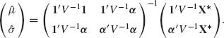
Let
![]()
and
![]()
then the BLUE can be written as
The variances and covariances of these BLUEs are
(5.4.17) 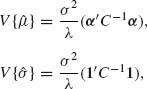
and
![]()
As will be illustrated in the following example the proposed BLUE, based on all the n order statistics, becomes impractical in certain situations.
Example 5.11 illustrates an estimation problem for which the BLUE based on all the n order statistics can be determined only numerically, provided the sample is not too large. Various methods have been developed to approximate the BLUEs by linear combinations of a small number of selected order statistics. Asymptotic (large sample) theory has been applied in the theory leading to the optimal choice of selected set of k, k < n, order statistics. This choice of order statistics is also called spacing. For the theories and methods used for the determination of the optimal spacing see the book of Sarhan and Greenberg (1962).
5.5 STABILIZING THE LSE: RIDGE REGRESSIONS
The method of ridge regression was introduced by Hoerl (1962) and by Hoerl and Kennard (1970). A considerable number of papers have been written on the subject since then. In particular see the papers of Marquardt (1970), Stone and Conniffe (1973), and others. The main objective of the ridge regression method is to overcome a phenomenon of possible instability of least–squares estimates, when the matrix of coefficients S = A′A has a large spread of the eigenvalues. To be more specific, consider again the linear model of full rank: X = Aβ + ![]() , where E{
, where E{![]() } = 0 and
} = 0 and ![]() , (
, (![]() ) = σ2I. We have seen that the LSE of β,
) = σ2I. We have seen that the LSE of β, ![]() = S−1A′X, minimizes the squared distance between the observed random vector X and the estimate of its expectation Aβ, i.e., ||X – AB||2. ||a|| denotes the Euclidean length of the vector a, i.e., ||a|| =
= S−1A′X, minimizes the squared distance between the observed random vector X and the estimate of its expectation Aβ, i.e., ||X – AB||2. ||a|| denotes the Euclidean length of the vector a, i.e., ||a|| =  . As we have shown in Section 5.3.2, the LSE in the present model is BLUE of β. However, if A is ill–conditioned, in the sense that the positive definite matrix S = A′A has large spread of the eigenvalues, with some being close to zero, then the LSE
 ![]() may be with high probability very far from β. Indeed, if L2 = ||
may be with high probability very far from β. Indeed, if L2 = ||![]() – β ||2 then
– β ||2 then
(5.5.1) ![]()
Let P be an orthogonal matrix that diagonalizes S, i.e., PSP′ = Λ, where Λ is a diagonal matrix consisting of the eigenvalues (λ1, …, λp) of S (all positive). Accordingly
(5.5.2) ![]()
We see that E{L2} ≥ ![]() , where λmin is the smallest eigenvalue. A very large value of E{L2} means that at least one of the components of β has a large variance. This implies that the corresponding value of βi may with high probability be far from the true value. The matrix A in experimental situations often represents the levels of certain factors and is generally under control of the experimenter. A good design will set the levels of the factors so that the columns of A will be orthogonal. In this case S = I, λ1 = … = λp = 1 and E{L2} attains the minimum possible value pσ2 for the LSE. In many practical cases, however, X is observed with an ill–conditioned coefficient matrix A. In this case, all the unbiased estimators of β are expected to have large values of L2. The way to overcome this deficiency is to consider biased estimators of β which are not affected strongly by small eigenvalues. Hoerl (1962) suggested the class of biased estimators
, where λmin is the smallest eigenvalue. A very large value of E{L2} means that at least one of the components of β has a large variance. This implies that the corresponding value of βi may with high probability be far from the true value. The matrix A in experimental situations often represents the levels of certain factors and is generally under control of the experimenter. A good design will set the levels of the factors so that the columns of A will be orthogonal. In this case S = I, λ1 = … = λp = 1 and E{L2} attains the minimum possible value pσ2 for the LSE. In many practical cases, however, X is observed with an ill–conditioned coefficient matrix A. In this case, all the unbiased estimators of β are expected to have large values of L2. The way to overcome this deficiency is to consider biased estimators of β which are not affected strongly by small eigenvalues. Hoerl (1962) suggested the class of biased estimators
(5.5.3) ![]()
with k ≥ 0, called the ridge regression estimators. It can be shown for every k > 0, ![]() *(k) has smaller length than the LSE
*(k) has smaller length than the LSE ![]() , i.e., ||
, i.e., ||![]() *(k)|| < ||
*(k)|| < ||![]() ||. The ridge estimator is compared to the LSE. If we graph the values of
||. The ridge estimator is compared to the LSE. If we graph the values of ![]() (k) as functions of k we often see that the estimates are very sensitive to changes in the values of k close to zero, while eventually as k grows the estimates stabilize. The graphs of
(k) as functions of k we often see that the estimates are very sensitive to changes in the values of k close to zero, while eventually as k grows the estimates stabilize. The graphs of ![]() (k) for i = 1, …, k are called the ridge trace. It is recommended by Hoerl and Kennard (1970) to choose the value of k at which the estimates start to stabilize.
(k) for i = 1, …, k are called the ridge trace. It is recommended by Hoerl and Kennard (1970) to choose the value of k at which the estimates start to stabilize.
Among all (biased) estimators B of β that lie at a fixed distance from the origin the ridge estimator β*(k), for a proper choice of k, minimizes the residual sum of squares ||X – AB||2. For proofs of these geometrical properties, see Hoerl and Kennard (1970). The sum of mean–squared errors (MSEs) of the components of ![]() *(k) is
*(k) is
(5.5.4) ![]()
where γ = Hβ and H is the orthogonal matrix diagonalizing A′A. E{L2(k)} is a differentiable function of k, having a unique minimum k(0)(γ). Moreover, E{L2(k0(β))} < E{L2(0)}, where E{L2(0)} is the sum of variances of the LSE components, as in (5.4.2). The problem is that the value of k0(γ) depends on γ and if k is chosen too far from k0(γ), E{L2(k)} may be greater than E{L2(0)}. Thus, a crucial problem in applying the ridge–regression method is the choice of a flattening factor k. Hoerl, Kennard, and Baldwin (1975) studied the characteristics of the estimator obtained by substituting in (5.4.3) an estimate of the optimal k0(γ). They considered the estimator
where ![]() is the LSE and
is the LSE and ![]() 2 is the estimate of the variance around the regression line, as in (5.4.11). The estimator
2 is the estimate of the variance around the regression line, as in (5.4.11). The estimator ![]() *(
*(![]() ) is not linear in X, since k is a nonlinear function of X. Most of the results proven for a fixed value of k do not necessarily hold when k is random, as in (5.5.5). For this reason Hoerl, Kennard, and Baldwin performed extensive simulation experiments to obtain estimates of the important characteristics of
) is not linear in X, since k is a nonlinear function of X. Most of the results proven for a fixed value of k do not necessarily hold when k is random, as in (5.5.5). For this reason Hoerl, Kennard, and Baldwin performed extensive simulation experiments to obtain estimates of the important characteristics of ![]() *(
*(![]() ). They found that with probability greater than 0.5 the ridge–type estimator
). They found that with probability greater than 0.5 the ridge–type estimator ![]() *(
*(![]() ) is closer (has smaller distance norm) to the true β than the LSE. Moreover, this probability increases as the dimension p of the factor space increases and as the spread of the eigenvalues of S increases. The ridge type estimator
) is closer (has smaller distance norm) to the true β than the LSE. Moreover, this probability increases as the dimension p of the factor space increases and as the spread of the eigenvalues of S increases. The ridge type estimator ![]() *(
*(![]() ) are similar to other types of nonlinear estimators (James – Stein, Bayes, and other types) designed to reduce the MSE. These are discussed in Chapter 8.
) are similar to other types of nonlinear estimators (James – Stein, Bayes, and other types) designed to reduce the MSE. These are discussed in Chapter 8.
A more general class of ridge–type estimators called the generalized ridge regression estimators is given by
(5.5.6) ![]()
where C is a positive definite matrix chosen so that A′A + C is nonsingular. [The class is actually defined also for A′A + C singular with a Moore – Penrose generalized inverse replacing (A′A + C)−1; see Marquardt (1970).]
5.6 MAXIMUM LIKELIHOOD ESTIMATORS
5.6.1 Definition and Examples
In Section 3.3, we introduced the notion of the likelihood function, L(θ;x) defined over a parameter space Θ, and studied some of its properties. We develop here an estimation theory based on the likelihood function.
The maximum likelihood estimator (MLE) of θ is a value of θ at which the likelihood function L(θ;x) attains its supremum (or maximum). We remark that if the family ![]() admits a nontrivial sufficient statistic T(X) then the MLE is a function of T(X). This is implied immediately from the Neyman – Fisher Factorization Theorem. Indeed, in this case,
admits a nontrivial sufficient statistic T(X) then the MLE is a function of T(X). This is implied immediately from the Neyman – Fisher Factorization Theorem. Indeed, in this case,
![]()
where h(x) > 0 with probability one. Hence, the kernel of the likelihood function can be written as L*(θ;x) = g(T(x);θ). Accordingly, the value θ that maximizes it depends on T(X). We also notice that although the MLE is a function of the sufficient statistic, the converse is not always true. An MLE is not necessarily a sufficient statistic.
5.6.2 MLEs in Exponential Type Families
Let X1, …, Xn be i.i.d. random variables having a k–parameter exponential type family, with a p.d.f. of the form (2.16.2). The likelihood function of the natural parameters is
(5.6.1) 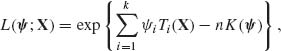
where
![]()
The MLEs of ![]() 1, …,
1, …, ![]() k are obtained by solving the system of k equations
k are obtained by solving the system of k equations
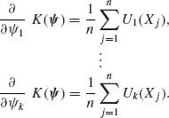
Note that whenever the expectations exist, E![]() {Ui(X)} = ∂ K(
{Ui(X)} = ∂ K(![]() )/∂
)/∂ ![]() i for each i = 1, …, k. Hence, if X1, …, Xn are i.i.d. E
i for each i = 1, …, k. Hence, if X1, …, Xn are i.i.d. E![]()
![]() , for each i = 1, …, k, where
, for each i = 1, …, k, where ![]() is the vector of MLEs. For all points
is the vector of MLEs. For all points ![]() in the interior of the parameter space n, the matrix
in the interior of the parameter space n, the matrix ![]() exists and is positive definite for all
exists and is positive definite for all ![]() since K(
since K(![]() ) is convex. Thus, the root
) is convex. Thus, the root ![]() of (5.6.2) is unique and is a m.s.s.
of (5.6.2) is unique and is a m.s.s.
5.6.3 The Invariance Principle
If the vector θ = (θ1, …, θk) is reparametrized by a one–to–one transformation ![]() 1 = g1(θ), …,
1 = g1(θ), …, ![]() k = gk(θ) then the MLEs of
k = gk(θ) then the MLEs of ![]() i are obtained by substituting in the g–functions the MLEs of θ. This is obviously true when the transformation θ →
i are obtained by substituting in the g–functions the MLEs of θ. This is obviously true when the transformation θ → ![]() is one–to–one. Indeed, if θ1 =
is one–to–one. Indeed, if θ1 = ![]() then the likelihood function L(θ;x) can be expressed as a function of
then the likelihood function L(θ;x) can be expressed as a function of ![]() ,
, ![]() . If (
. If (![]() 1, …,
1, …, ![]() k) is a point at which L(θ, x) attains its supremum, and if
k) is a point at which L(θ, x) attains its supremum, and if ![]() = (g1(
= (g1(![]() ), …, gk(
), …, gk(![]() )) then, since the transformation is one–to–one,
)) then, since the transformation is one–to–one,
(5.6.3) ![]()
where L*(![]() ;x) is the likelihood, as a function of
;x) is the likelihood, as a function of ![]() . This result can be extended to general transformations, not necessarily one–to–one, by a proper redefinition of the concept of MLE over the space of the
. This result can be extended to general transformations, not necessarily one–to–one, by a proper redefinition of the concept of MLE over the space of the ![]() –values. Let
–values. Let ![]() = g(θ) be a vector valued function of θ; i.e.,
= g(θ) be a vector valued function of θ; i.e., ![]() = g(θ) = (g1(θ), …, gk(θ)) where the dimension of g(θ), r, does not exceed that of θ, k.
= g(θ) = (g1(θ), …, gk(θ)) where the dimension of g(θ), r, does not exceed that of θ, k.
Following Zehna (1966), we introduce the notion of the profile likelihood function of ![]() = (
= (![]() 1, …,
1, …, ![]() r). Define the cosets of θ–values
r). Define the cosets of θ–values
(5.6.4) ![]()
and let L(θ;x) be the likelihood function of θ given X. The profile likelihood of ![]() given X is defined as
given X is defined as
(5.6.5) ![]()
Obviously, in the one–to–one case L*(θ;x) = ![]() . Generally, we define the MLE of
. Generally, we define the MLE of ![]() to be the value at which L*(
to be the value at which L*(![]() ; x) attains its supremum. It is easy then to prove that if
; x) attains its supremum. It is easy then to prove that if ![]() is an MLE of θ and
is an MLE of θ and ![]() = g(
= g(![]() ), then
), then ![]() is an MLE of
is an MLE of ![]() , i.e.,
, i.e.,
(5.6.6) ![]()
5.6.4 MLE of the Parameters of Tolerance Distributions
Suppose that k–independent experiments are performed at controllable real–valued experimental levels (dosages) -∞ < x1 < … < xk < ∞. At each of these levels nj Bernoulli trials are performed (j = 1, …, k). The success probabilities of these Bernoulli trials are increasing functions F(x) of x. These functions, called tolerance distributions, are the expected proportion of (individuals) units in a population whose tolerance against the applied dosage does not exceed the level x. The model thus consists of k–independent random variables J1, …, Jk such that Ji ∼ B(ni, F(xi;θ)), i = 1, …, k, where θ = (θ1, …, θr), 1 ≤ r < k, is a vector of unknown parameters. The problem is to estimate θ. Frequently applied models are
(5.6.7) 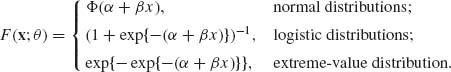
We remark that in some of the modern literature the tolerance distributions are called link functions (see Lindsey, 1996). Generally, if F(α + βxi) is the success probability at level xi, the likelihood function of (α, β), given J1, …, Jk and x1, …, xk, n1, …, nk, is
(5.6.8) 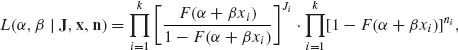
and the log–likelihood function is

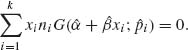
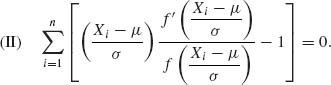
The MLE of α and β are the roots of the nonlinear equations
(5.6.9) 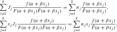
where f(z) = F′(z) is the p.d.f. of the standardized distribution F(z) and ![]() (z) = 1 – F(z).
(z) = 1 – F(z).
Let ![]() i = Ji/ni, i = 1, …, k, and define the function
i = Ji/ni, i = 1, …, k, and define the function
Accordingly, the MLEs of α and β are the roots ![]() and
and ![]() of the equations
of the equations
(5.6.11) 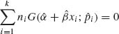
and
The solution of this system of (generally nonlinear) equations according to the Newton – Raphson method proceeds as follows. Let ![]() 0 and
0 and ![]() 0 be an initial solution. The adjustment after the jth iteration (j = 0, 1, …) is
0 be an initial solution. The adjustment after the jth iteration (j = 0, 1, …) is ![]() j + 1 =
j + 1 = ![]() j + δ αj and
j + δ αj and ![]() j + 1 =
j + 1 = ![]() j + δ βj, where δ αj and δ βj are solutions of the linear equations
j + δ βj, where δ αj and δ βj are solutions of the linear equations
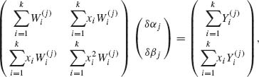
where
(5.6.13) ![]()
and
![]()
and G′(z;![]() ) =
) = ![]() . The linear equations (5.6.12) resemble the normal equations in weighted least–squares estimation. However, in the present problems the weights depend on the unknown parameters α and β. In each iteration, the current estimates of α and β are substituted. For applications of this procedure in statistical reliability and bioassay quantal response analysis, see Finney (1964), Gross and Clark (1975), and Zacks (1997).
. The linear equations (5.6.12) resemble the normal equations in weighted least–squares estimation. However, in the present problems the weights depend on the unknown parameters α and β. In each iteration, the current estimates of α and β are substituted. For applications of this procedure in statistical reliability and bioassay quantal response analysis, see Finney (1964), Gross and Clark (1975), and Zacks (1997).
5.7 EQUIVARIANT ESTIMATORS
5.7.1 The Structure of Equivariant Estimators
Certain families of distributions have structural properties that are preserved under transformations of the random variables. For example, if X has an absolutely continuous distribution belonging to a family ![]() which depends on location and scale parameters, i.e., its p.d.f. is f(x;μ, σ) =
which depends on location and scale parameters, i.e., its p.d.f. is f(x;μ, σ) = ![]() , where -∞ < μ < ∞ and 0 < σ < ∞, then any real–affine transformation of X, given by
, where -∞ < μ < ∞ and 0 < σ < ∞, then any real–affine transformation of X, given by
![]()
yields a random variable Y = α + β X with p.d.f. f(y;μ, σ) = ![]() , where
, where ![]() = α + β μ and
= α + β μ and ![]() = β σ. Thus, the distribution of Y belongs to the same family
= β σ. Thus, the distribution of Y belongs to the same family ![]() . The family
. The family ![]() is preserved under transformations belonging to the group
is preserved under transformations belonging to the group ![]() = {[α, β]; -∞ < α < ∞, 0 < β < ∞ } of real–affine transformations.
= {[α, β]; -∞ < α < ∞, 0 < β < ∞ } of real–affine transformations.
In this section, we present the elements of the theory of families of distributions and corresponding estimators having structural properties that are preserved under certain groups of transformations. For a comprehensive treatment of the theory and its geometrical interpretation, see the book of Fraser (1968). Advanced treatment of the subject can be found in Berk (1967), Hall, Wijsman, and Ghosh (1965), Wijsman (1990), and Eaton (1989). We require that every element g of ![]() be a one–to–one transformation of
be a one–to–one transformation of ![]() onto
onto ![]() . Accordingly, the sample space structure does not change under these transformations. Moreover, if
. Accordingly, the sample space structure does not change under these transformations. Moreover, if ![]() is the Borel σ–field on
is the Borel σ–field on ![]() then, for all g
then, for all g ![]()
![]() , we require that Pθ [gB] will be well defined for all B
, we require that Pθ [gB] will be well defined for all B ![]()
![]() and θ
and θ ![]() Θ. Furthermore, as seen in the above example of the location and scale parameter distributions, if θ is a parameter of the distribution of X the parameter of Y = gX is
Θ. Furthermore, as seen in the above example of the location and scale parameter distributions, if θ is a parameter of the distribution of X the parameter of Y = gX is ![]() θ, where
θ, where ![]() is a transformation on the parameter space Θ defined by the relationship
is a transformation on the parameter space Θ defined by the relationship
(5.7.1) ![]()
In the example of real–affine transformations, if g = [α, β] and θ = (μ, σ), then ![]() (μ, σ) = (α + β μ, β σ). We note that
(μ, σ) = (α + β μ, β σ). We note that ![]() Θ = Θ for every
Θ = Θ for every ![]() corresponding to g in
corresponding to g in ![]() . Suppose that X1, …, Xn are i.i.d. random variables whose distribution F belongs to a family
. Suppose that X1, …, Xn are i.i.d. random variables whose distribution F belongs to a family ![]() that is preserved under transformations belonging to a group
that is preserved under transformations belonging to a group ![]() . If T(X1, …, Xn) is a statistic, then we define the transformations
. If T(X1, …, Xn) is a statistic, then we define the transformations ![]() on the range
on the range ![]() of T(X1, …, Xn), corresponding to transformations g of
of T(X1, …, Xn), corresponding to transformations g of ![]() , by
, by
(5.7.2) ![]()
A statistic S(X1, …, Xn) is called invariant with respect to ![]() if
if
(5.7.3) ![]()
A coset of x0 with respect to ![]() is the set of all points that can be obtained as images of x0, i.e.,
is the set of all points that can be obtained as images of x0, i.e.,
![]()
Such a coset is called also an orbit of ![]() in
in ![]() through x0. If x0 = (x01, …, x0n) is a given vector, the orbit of
through x0. If x0 = (x01, …, x0n) is a given vector, the orbit of ![]() in
in ![]() (n) through x0 is the coset
(n) through x0 is the coset
![]()
If x(1) and x(2) belong to the same orbit and S(x) = S(x1, …, xn) is invariant with respect to ![]() then S(x(1)) = S(x(2)). A statistic U(X) = U(X1, …, Xn) is called maximal invariant if it is invariant and if X(1) and X(2) belong to two different orbits then U(X(1)) ≠ U(X(2)). Every invariant statistic is a function of a maximal invariant statistic.
then S(x(1)) = S(x(2)). A statistic U(X) = U(X1, …, Xn) is called maximal invariant if it is invariant and if X(1) and X(2) belong to two different orbits then U(X(1)) ≠ U(X(2)). Every invariant statistic is a function of a maximal invariant statistic.
If ![]() (X1, …, Xn) is an estimator of θ, it would be often desirable to have the property that the estimator reacts to transformations of
(X1, …, Xn) is an estimator of θ, it would be often desirable to have the property that the estimator reacts to transformations of ![]() in the same manner as the parameters θ do, i.e.,
in the same manner as the parameters θ do, i.e.,
5.7.2 Minimum MSE Equivariant Estimators
Estimators satisfying (5.7.4) are called equivariant. The objective is to derive an equivariant estimator having a minimum MSE or another optimal property. The algebraic structure of the problem allows us often to search for such optimal estimators in a systematic manner.
5.7.3 Minimum Risk Equivariant Estimators
A loss function L(![]() (X), θ) is called invariant under
(X), θ) is called invariant under ![]() if
if
(5.7.5) ![]()
for all θ ![]() Θ and all g
Θ and all g ![]()
![]() .
.
The coset C(θ0) = {θ;θ = ![]() θ0, g
θ0, g ![]()
![]() } is called an orbit of
} is called an orbit of ![]() through θ0 in Θ. We show now that if
through θ0 in Θ. We show now that if ![]() (X) is an equivariant estimator and L(
(X) is an equivariant estimator and L(![]() (X), θ) is an invariant loss function then the risk function R(
(X), θ) is an invariant loss function then the risk function R(![]() , θ) = E{L(
, θ) = E{L(![]() (X), θ)} is constant on each orbit of
(X), θ)} is constant on each orbit of ![]() in Θ. Indeed, for any g
in Θ. Indeed, for any g ![]()
![]() , if the distribution of X is F(x;θ) and the distribution of Y = gX is F(y;
, if the distribution of X is F(x;θ) and the distribution of Y = gX is F(y;![]() θ), then if
θ), then if ![]() is equivariant
is equivariant
(5.7.6) 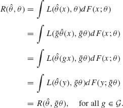
Thus, whenever the structure of the model is such that Θ contains only one orbit with respect to ![]() , and there exist equivariant estimators with finite risk, then each such equivariant estimator has a constant risk function. In Example 5.23, we illustrate such cases. We consider there the location and scale parameter family of the normal distributions N(μ, σ). This family has a parameter space Θ, which has only one orbit with respect to the group
, and there exist equivariant estimators with finite risk, then each such equivariant estimator has a constant risk function. In Example 5.23, we illustrate such cases. We consider there the location and scale parameter family of the normal distributions N(μ, σ). This family has a parameter space Θ, which has only one orbit with respect to the group ![]() of real–affine transformations. If the parameter space has various orbits, as in the case of Example 5.24, there is no global uniformly minimum risk equivariant estimator, but only locally for each orbit. In Example 5.26, we construct uniformly minimum risk equivariant estimators of the scale and shape parameters of Weibull distributions for a group of transformations and a corresponding invariant loss function.
of real–affine transformations. If the parameter space has various orbits, as in the case of Example 5.24, there is no global uniformly minimum risk equivariant estimator, but only locally for each orbit. In Example 5.26, we construct uniformly minimum risk equivariant estimators of the scale and shape parameters of Weibull distributions for a group of transformations and a corresponding invariant loss function.
5.7.4 The Pitman Estimators
We develop here the minimum MSE equivariant estimators for the special models of location parameters and location and scale parameters. These estimators are called the Pitman estimators.
Consider first the family ![]() of location parameters distributions, i.e., every p.d.f. of
of location parameters distributions, i.e., every p.d.f. of ![]() is given by f(x;θ) =
is given by f(x;θ) = ![]() (x-θ), -∞ < θ < ∞.
(x-θ), -∞ < θ < ∞. ![]() (x) is the standard p.d.f. According to our previous discussion, we consider the group
(x) is the standard p.d.f. According to our previous discussion, we consider the group ![]() of real translations. Let
of real translations. Let ![]() (X) be an equivariant estimator of θ. Then, writing T = (
(X) be an equivariant estimator of θ. Then, writing T = (![]() , X(1)-
, X(1)-![]() , …, X(n)-
, …, X(n)-![]() ), where X(1) ≤ … ≤ X(n), for any equivariant estimator, d(X), of θ, we have
), where X(1) ≤ … ≤ X(n), for any equivariant estimator, d(X), of θ, we have
![]()
Note that U = (X(1) – ![]() , …, X(n) –
, …, X(n) – ![]() has a distribution that does not depend on θ. Moreover, since
has a distribution that does not depend on θ. Moreover, since ![]() (X) is an equivariant estimator, we can write
(X) is an equivariant estimator, we can write
![]()
Thus, the MSE of d(X) is
(5.7.7) ![]()
It follows immediately that the function ![]() (U) which minimizes the MSE is the conditional expectation
(U) which minimizes the MSE is the conditional expectation
(5.7.8) ![]()
Thus, the minimum MSE equivariant estimator is
This is a generalized form of the Pitman estimator. The well–known specific form of the Pitman estimator is obtained by starting with ![]() (X) = X(1). In this case, F(Y) = Y(1), where Y(1) is the minimum of a sample from a standard distribution. Formula (5.7.9) is then reduced to the special form
(X) = X(1). In this case, F(Y) = Y(1), where Y(1) is the minimum of a sample from a standard distribution. Formula (5.7.9) is then reduced to the special form
(5.7.10) 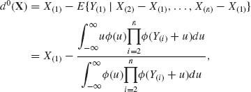
where Y(i) = X(i) – X(1), i = 2, …, n. In the derivation of (5.7.9), we have assumed that the MSE of d(X) exists. A minimum risk equivariant estimator may not exist. Finally, we mentioned that the minimum MSE equivariant estimators are unbiased. Indeed
(5.7.11) ![]()
If ![]() is a scale and location family of distribution, with p.d.f.s of the form
is a scale and location family of distribution, with p.d.f.s of the form
![]()
where ![]() (u) is a p.d.f., then every equivariant estimator of μ with respect to the group
(u) is a p.d.f., then every equivariant estimator of μ with respect to the group ![]() of real–affine transformations can be expressed in the form
of real–affine transformations can be expressed in the form
(5.7.12) ![]()
where X(1) ≤ … ≤ X(n) is the order statistic, X(2) – X(1) > 0 and Z = (Z3, …, Zn)′, with Zi = (X(i) – X(1))/(X(2) – X(1)). The MSE of ![]() (X) is given by
(X) is given by
(5.7.13) 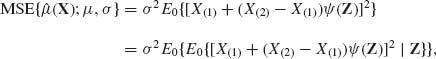
where E0{·} designates an expectation with respect to the standard distribution (μ = 0, σ = 1). An optimal choice of ![]() (Z) is such for which E0{[X(1) + (X(2) – X(1))
(Z) is such for which E0{[X(1) + (X(2) – X(1))![]() (Z)]2| Z} is minimal. Thus, the minimum MSE equivariant estimator of μ is
(Z)]2| Z} is minimal. Thus, the minimum MSE equivariant estimator of μ is
(5.7.14) ![]()
where
(5.7.15) ![]()
Equivalently, the Pitman estimator of the location parameter is expressed as
(5.7.16) 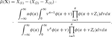
In a similar manner, we show that the minimum MSE equivariant estimator for σ is ![]() 0(Xn) = (X(2)-X(1))
0(Xn) = (X(2)-X(1))![]() 0(Z3, …, Zn), where
0(Z3, …, Zn), where
(5.7.17) ![]()
Indeed, ![]() 0(Z) minimizes E0{(U2
0(Z) minimizes E0{(U2![]() (Z) – 1)2| Z}. Accordingly, the Pitman estimator of the scale parameter, σ, is
(Z) – 1)2| Z}. Accordingly, the Pitman estimator of the scale parameter, σ, is
(5.7.18) 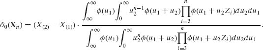
5.8 ESTIMATING EQUATIONS
5.8.1 Moment–Equations Estimators
Suppose that ![]() is a family of distributions depending on k real parameters, θ1, …, θk, 1 ≤ k. Suppose that the moments μr, 1 ≤ r ≤ k, exist and are given by some specified functions
is a family of distributions depending on k real parameters, θ1, …, θk, 1 ≤ k. Suppose that the moments μr, 1 ≤ r ≤ k, exist and are given by some specified functions
![]()
If X1, …, Xn are i.i.d. random variables having a distribution in ![]() , the sample moments Mr =
, the sample moments Mr = ![]() are unbiased estimators of μ r (1 ≤ r ≤ k) and by the laws of large numbers (see Section 1.11) they converge almost surely to μr as n → ∞. The roots of the system of equations
are unbiased estimators of μ r (1 ≤ r ≤ k) and by the laws of large numbers (see Section 1.11) they converge almost surely to μr as n → ∞. The roots of the system of equations
(5.8.1) ![]()
are called the moment–equations estimators (MEEs) of θ1, …, θk.
In Examples 5.28 – 5.29, we discuss cases where both the MLE and the MEE can be easily determined, but the MLE exhibiting better characteristics. The question is then, why should we consider the MEEs at all? The reasons for considering MEEs are as follows:
5.8.2 General Theory of Estimating Functions
Both the MLE and the MME are special cases of a class of estimators called estimating functions estimator. A function g(X;θ), X ![]()
![]() (n) and θ
(n) and θ ![]() Θ, is called an estimating function, if the root
Θ, is called an estimating function, if the root ![]() (X) of the equation
(X) of the equation
belongs to Θ; i.e., ![]() (X) is an estimator of θ. Note that if θ is a k–dimensional vector then (5.8.2) is a system of k–independent equations in θ. In other words, g(X, θ) is a k–dimensional vector function, i.e.,
(X) is an estimator of θ. Note that if θ is a k–dimensional vector then (5.8.2) is a system of k–independent equations in θ. In other words, g(X, θ) is a k–dimensional vector function, i.e.,
![]()
![]() (X) is the simultaneous solution of
(X) is the simultaneous solution of
(5.8.3) 
In the MEE case, gi(X, θ) = Mi(θ1, …, θk) – mi (i = 1, …, k). In the MLE case,
![]()
In both cases, Eθ{g(X, θ)} = 0 for all θ, under the CR regularity conditions (see Theorem 5.2.2).
An estimating function g(X, θ) is called unbiased if Eθ {g(X;θ)} = 0 for all θ. The information in an estimating function g(X, θ) is defined as
(5.8.4) 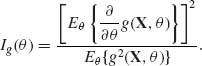
For example, if g(X, θ) is the score function S(X, θ), then under the regularity conditions (3.7.2), ![]() = -I(θ) and Eθ {S2(X;θ)} = I(θ), where I(θ) is the Fisher information function. A basic result of is that Ig(θ) ≤ I(θ) for all unbiased estimating functions.
= -I(θ) and Eθ {S2(X;θ)} = I(θ), where I(θ) is the Fisher information function. A basic result of is that Ig(θ) ≤ I(θ) for all unbiased estimating functions.
The CR regularity conditions are now generalized for estimating functions. The regularity conditions for estimating functions are as follows:
Let T be a sufficient statistic for a parametric family ![]() . Bhapkar (1972) proved that, for any unbiased estimating function g, if
. Bhapkar (1972) proved that, for any unbiased estimating function g, if
![]()
then Ig(θ) ≤ Ig* (θ) for all θ with equality if and only if g* ![]()
![]() T. This is a generalization of the Blackwell – Rao Theorem to unbiased estimating functions. Under the regularity conditions, the score function S(X, θ) =
T. This is a generalization of the Blackwell – Rao Theorem to unbiased estimating functions. Under the regularity conditions, the score function S(X, θ) = ![]() log f(X, θ) depends on X only through the likelihood statistic T(X), which is minimal sufficient. Thus, the score function is most informative among the unbiased estimating functions that satisfy the regularity conditions. If θ is a vector parameter, then the information in g is
log f(X, θ) depends on X only through the likelihood statistic T(X), which is minimal sufficient. Thus, the score function is most informative among the unbiased estimating functions that satisfy the regularity conditions. If θ is a vector parameter, then the information in g is
where
(5.8.6) ![]()
and
(5.8.7) ![]()
where g(X, θ) = (g1(X, θ), …, gk(X, θ))′ is a vector of k estimating functions, for estimating the k components of θ.
We can show that I(θ) = Ig(θ) is a nonnegative definite matrix, and I(θ) is the Fisher information matrix.
Various applications of the theory of estimating functions can be found in Godambe (1991).
5.9 PRETEST ESTIMATORS
Pretest estimators (PTEs) are estimators of the parameters, or functions of the parameters of a distribution, which combine testing of some hypothesis (es) and estimation for the purpose of reducing the MSE of the estimator. The idea of preliminary testing has been employed informally in statistical methodology in many different ways and forms. Statistical inference is often based on some model, which assumes a certain set of assumptions. If the model is correct, or adequately fits the empirical data, the statistician may approach the problem of estimating the parameters of interest in a certain manner. However, if the model is rejectable by the data the estimation of the parameter of interest may have to follow a different procedure. An estimation procedure that assumes one of two alternative forms, according to the result of a test of some hypothesis, is called a pretest estimation procedure.
PTEs have been studied in various estimation problems, in particular in various least–squares estimation problems for linear models. As we have seen in Section 4.6, if some of the parameters of a linear model can be assumed to be zero (or negligible), the LSE should be modified, according to formula (4.6.14). Accordingly, if ![]() denotes the unconstrained LSE of a full–rank model and β* the constrained LSE (4.6.14), the PRE of β is
denotes the unconstrained LSE of a full–rank model and β* the constrained LSE (4.6.14), the PRE of β is
(5.9.1) ![]()
where A denotes the acceptance set of the hypothesis H0: βr + 1 = βr + 2 = … = β p = 0; and ![]() the complement of A. An extensive study of PREs for linear models, of the form (5.8.5), is presented in the book of Judge and Bock (1978). The reader is referred also to the review paper of Billah and Saleh (1998).
the complement of A. An extensive study of PREs for linear models, of the form (5.8.5), is presented in the book of Judge and Bock (1978). The reader is referred also to the review paper of Billah and Saleh (1998).
5.10 ROBUST ESTIMATION OF THE LOCATION AND SCALE PARAMETERS OF SYMMETRIC DISTRIBUTIONS
In this section, we provide some new developments concerning the estimation of the location parameter, μ, and the scale parameter, σ, in a parametric family, ![]() , whose p.d.f.s are of the form f(x;μ, σ) =
, whose p.d.f.s are of the form f(x;μ, σ) = ![]() , and f(-x) = f(x) for all -∞ < x < ∞. We have seen in various examples before that an estimator of μ, or of σ, which has small MSE for one family may not be as good for another. We provide below some variance comparisons of the sample mean,
, and f(-x) = f(x) for all -∞ < x < ∞. We have seen in various examples before that an estimator of μ, or of σ, which has small MSE for one family may not be as good for another. We provide below some variance comparisons of the sample mean, ![]() , and the sample median, Me, for the following families: normal, mixture of normal and rectangular, t[ν], Laplace and Cauchy. The mixtures of normal and rectangular distributions will be denoted by (1 – α)N + α R(-3σ, 3σ). Such a family of mixtures has the standard density function
, and the sample median, Me, for the following families: normal, mixture of normal and rectangular, t[ν], Laplace and Cauchy. The mixtures of normal and rectangular distributions will be denoted by (1 – α)N + α R(-3σ, 3σ). Such a family of mixtures has the standard density function
![]()
The t[ν] distributions have a standard p.d.f. as given in (2.13.5). The asymptotic (large sample) variance of the sample median, Me, is given by the formula (7.9.3)
(5.10.1) ![]()
provided f(0) > 0, and f(x) is continuous at x = 0.
Table 5.1 Asymptotic Variances of ![]() and Me
and Me
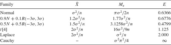
In Table 5.1, we provide the asymptotic variances of ![]() and Me and their ratio E = AV{
and Me and their ratio E = AV{![]() }/AV{Me}, for the families mentioned above. We see that the sample mean
}/AV{Me}, for the families mentioned above. We see that the sample mean ![]() which is a very good estimator of the location parameter, μ, when
which is a very good estimator of the location parameter, μ, when ![]() is the family of normal distributions loses its efficiency when
is the family of normal distributions loses its efficiency when ![]() deviates from normality. The reason is that the sample mean is very sensitive to deviations in the sample of the extreme values. The sample mean performs badly when the sample is drawn from a distribution having heavy tails (relatively high probabilities of large deviations from the median of the distribution). This phenomenon becomes very pronounced in the case of the Cauchy family. One can verify (Fisz, 1963, p. 156) that if X1, …, Xn are i.i.d. random variables having a common Cauchy distribution than the sample mean
deviates from normality. The reason is that the sample mean is very sensitive to deviations in the sample of the extreme values. The sample mean performs badly when the sample is drawn from a distribution having heavy tails (relatively high probabilities of large deviations from the median of the distribution). This phenomenon becomes very pronounced in the case of the Cauchy family. One can verify (Fisz, 1963, p. 156) that if X1, …, Xn are i.i.d. random variables having a common Cauchy distribution than the sample mean ![]() has the same Cauchy distribution, irrespective of the sample size. Furthermore, the Cauchy distribution does not have moments, or we can say that the variance of
has the same Cauchy distribution, irrespective of the sample size. Furthermore, the Cauchy distribution does not have moments, or we can say that the variance of ![]() is infinite. In order to avoid such possibly severe consequences due to the use of
is infinite. In order to avoid such possibly severe consequences due to the use of ![]() as an estimator of μ, when the statistician specifies the model erroneously, several types of less sensitive estimators of μ and σ were developed. These estimators are called robust in the sense that their performance is similar, in terms of the sampling variances and other characteristics, over a wide range of families of distributions. We provide now a few such robust estimators of the location parameter:
as an estimator of μ, when the statistician specifies the model erroneously, several types of less sensitive estimators of μ and σ were developed. These estimators are called robust in the sense that their performance is similar, in terms of the sampling variances and other characteristics, over a wide range of families of distributions. We provide now a few such robust estimators of the location parameter:
(5.10.2) ![]()
The median, Me is a special case, when α → 0.5.
(5.10.3) ![]()
Another such estimator is called the trimean and is given by
![]()
(5.10.4) 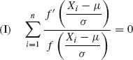
and
In analogy to the MLE solution and, in order to avoid strong dependence on a particular form of f(x), a general class of M–estimators is defined as the simultaneous solution of
(5.10.5) ![]()
and
![]()
for suitably chosen ![]() (·) and χ(·) functions. Huber (1964) proposed the M–estimators for which
(·) and χ(·) functions. Huber (1964) proposed the M–estimators for which
(5.10.6) 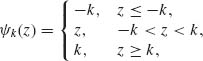
and
(5.10.7) ![]()
where
![]()
The determination of Huber’s M–estimators requires numerical iterative solutions. It is customary to start with the initial solution of μ = Me and σ = (Q3 – Q1)/1.35, where Q3 – Q1 is the interquartile range, or ![]() . Values of k are usually taken in the interval [1, 2].
. Values of k are usually taken in the interval [1, 2].
Other M–estimators were introduced by considering a different kind of ![]() (·) function. Having estimated the value of γ by
(·) function. Having estimated the value of γ by ![]() , use the estimator
, use the estimator
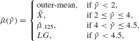
where the “outer–mean” is the mean of the extreme values in the sample. The reader is referred to the Princeton Study (Andrews et al., 1972) for a comprehensive examination of these and many other robust estimators of the location parameter. Another important article on the subject is that of Huber (1964, 1967).
Robust estimators of the scale parameter, σ, are not as well developed as those of the location parameter. The estimators that are used are
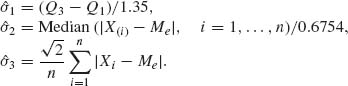
Further developments have been recently attained in the area of robust estimation of regression coefficients in multiple regression problems.
PART II: EXAMPLES
Example 5.1. In the production of concrete, it is required that the proportion of concrete cubes (of specified dimensions) having compressive strength not smaller than ξ0 be at least 0.95. In other words, if X is a random variable representing the compressive strength of a concrete cube, we require that P{X ≥ ξ0} = 0.95. This probability is a numerical characteristic of the distribution of X. Let X1, …, Xn be a sample of i.i.d. random variables representing the compressive strength of n randomly chosen cubes from the production process under consideration. If we do not wish to subject the estimation of p0 = P{X ≥ ξ0} to strong assumptions concerning the distribution of X we can estimate this probability by the proportion of cubes in the sample whose strength is at least ξ0; i.e.,
![]()
We note that n![]() has the binomial distribution B(n, p0). Thus, properties of the estimator
has the binomial distribution B(n, p0). Thus, properties of the estimator ![]() can be deduced from this binomial distribution.
can be deduced from this binomial distribution.
A commonly accepted model for the compressive strength is the family of log–normal distributions. If we are willing to commit the estimation procedure to this model we can obtain estimators of p0 which are more efficient than ![]() , provided the model is correct. Let Yi = log Xi, i = 1, …, and let
, provided the model is correct. Let Yi = log Xi, i = 1, …, and let ![]() n =
n = ![]() . Let η0 = log ξ0. Then, an estimator of p0 can be
. Let η0 = log ξ0. Then, an estimator of p0 can be
![]()
where Φ(u) is the standard normal c.d.f. Note that ![]() n and Sn are the sample statistics that are substituted to estimate the unknown parameters (ξ, σ). Moreover, (
n and Sn are the sample statistics that are substituted to estimate the unknown parameters (ξ, σ). Moreover, (![]() n, Sn) is a m.s.s. for the family of log–normal distributions. The estimator we have exhibited depends on the sample values only through the m.s.s. As will be shown later the estimator
n, Sn) is a m.s.s. for the family of log–normal distributions. The estimator we have exhibited depends on the sample values only through the m.s.s. As will be shown later the estimator ![]() has certain optimal properties in large samples, and even in small samples it is a reasonable estimator to use, provided the statistical model used is adequate for the real phenomenon at hand.
has certain optimal properties in large samples, and even in small samples it is a reasonable estimator to use, provided the statistical model used is adequate for the real phenomenon at hand. ![]()
Example 5.2. Let X1, …, Xn be i.i.d. random variables having a rectangular distribution R(0, θ), 0 < θ < ∞. Suppose that the characteristic of interest is the expectation μ = θ/2. The unbiased estimator ![]() =
= ![]() n has a variance
n has a variance
![]()
On the other hand, consider the m.s.s. X(n) = ![]() . The expected value of X(n) is
. The expected value of X(n) is
![]()
Hence, the estimator ![]() =
= ![]() is also an unbiased estimator of μ. The variance of
is also an unbiased estimator of μ. The variance of ![]() is
is
![]()
Thus, Vθ {![]() } < Vθ {
} < Vθ {![]() n} for all n ≥ 2, and
n} for all n ≥ 2, and ![]() is a better estimator than
is a better estimator than ![]() n. We note that
n. We note that ![]() depends on the m.s.s. X(n), while
depends on the m.s.s. X(n), while ![]() n is not a sufficient statistic. This is the main reason for the superiority of
n is not a sufficient statistic. This is the main reason for the superiority of ![]() over
over ![]() n. The theoretical justification is provided in the Rao – Blackwell Theorem.
n. The theoretical justification is provided in the Rao – Blackwell Theorem. ![]()
Example 5.3. Let X1, …, Xn be i.i.d. random variables having a common normal distribution, i.e., ![]() = {N(ξ, σ2); -∞ < ξ < ∞, 0 < σ < ∞ }. Both the mean ξ and the variance σ2 are unknown. We wish to estimate unbiasedly the probability g(ξ, σ) = Pξ, σ{X ≤ ξ0}. Without loss of generality, assume that ξ0 = 0, which implies that g(ξ, σ) = Φ (ξ /σ). Let
= {N(ξ, σ2); -∞ < ξ < ∞, 0 < σ < ∞ }. Both the mean ξ and the variance σ2 are unknown. We wish to estimate unbiasedly the probability g(ξ, σ) = Pξ, σ{X ≤ ξ0}. Without loss of generality, assume that ξ0 = 0, which implies that g(ξ, σ) = Φ (ξ /σ). Let ![]() n =
n = ![]() and
and ![]() be the sample mean and variance. (
be the sample mean and variance. (![]() , S2) is a complete sufficient statistic. According to the Rao – Blackwell Theorem, there exists an essentially unique unbiased estimator of Φ (ξ /σ) that is a function of the complete sufficient statistic. We prove now that this UMVU estimator is
, S2) is a complete sufficient statistic. According to the Rao – Blackwell Theorem, there exists an essentially unique unbiased estimator of Φ (ξ /σ) that is a function of the complete sufficient statistic. We prove now that this UMVU estimator is
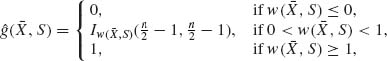
where
![]()
The proof is based on the following result (Ellison, 1964). If U and V are independent random variables ![]() and
and ![]() then
then![]() . Let ν = n – 1 and V =
. Let ν = n – 1 and V = ![]() . Accordingly
. Accordingly
![]()
where ![]() is independent of (
is independent of (![]() , S). Thus, by substituting in the expression for w(
, S). Thus, by substituting in the expression for w(![]() , S), we obtain
, S), we obtain
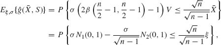
with N1(0, 1) and N2(0, 1) independent standard normal random variables. Thus,
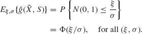
We provide an additional example that illustrates the Rao – Blackwellization method. ![]()
Example 5.4. Let X1, …, Xn be i.i.d. random variables, having a common Poisson distribution, P(λ), 0 < λ < ∞. We wish to estimate unbiasedly the Poisson probability p(k;λ) = e– λλk/k! An unbiased estimator of p(k;λ) based on one observation is
![]()
Obviously, this estimator is inefficient. According to the Rao – Blackwell Theorem the MVUE of p(k;λ) is
![]()
where Tn = ∑ Xi is the complete sufficient statistic. If Tn > 0 the conditional distribution of X1, given Tn is the binomial ![]() . Accordingly, the MVUE of p(k;λ) is
. Accordingly, the MVUE of p(k;λ) is
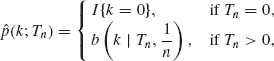
where ![]() is the p.d.f. of the Binomial distribution
is the p.d.f. of the Binomial distribution ![]() .
. ![]()
Example 5.5. We have seen in Section 3.6 that if the m.s.s. S(X) is incomplete, there is reason to find an ancillary statistic A(X) and base the inference on the conditional distribution of S(X), given A(X). We illustrate in the following example a case where such an analysis does not improve.
Let X1, …, Xn be i.i.d. random variables having a rectangular distribution in
![]()
A likelihood function for θ is
![]()
where X(1) < … < X(n) is the order statistic. A m.s.s. is (X(1), X(n)). This statistic, however, is incomplete. Indeed, ![]() , but
, but ![]() for each θ.
for each θ.
Writing R(θ – 1, θ + 1)∼ θ – 1 + 2R(0, 1) we have X(1) ∼ θ – 1 + 2U(1) and X(n) ∼ θ – 1 + 2U(n), where U(1) and U(n) are the order statistics from R(0, 1). Moreover, E{U(1)} = ![]() and E{U(n)} =
and E{U(n)} = ![]() . It follows immediately that
. It follows immediately that ![]() =
= ![]() (X(1) + X(n)) is unbiased. By the Blackwell – Rao Theorem it cannot be improved by conditioning on the sufficient statistic.
(X(1) + X(n)) is unbiased. By the Blackwell – Rao Theorem it cannot be improved by conditioning on the sufficient statistic.
We develop now the conditional distribution of ![]() , given the ancillary statistic W = X(n) – X(1). The p.d.f. of W is
, given the ancillary statistic W = X(n) – X(1). The p.d.f. of W is
![]()
The transformation (X(1), Xn → (![]() , W) is one to one. The joint p.d.f. of (
, W) is one to one. The joint p.d.f. of (![]() , W) is
, W) is
![]()
Accordingly,
![]()
That is, ![]() | W ∼ R
| W ∼ R![]() . Thus,
. Thus,
![]()
and
![]()
We have seen already that ![]() is an unbiased estimator. From the law of total variance, we get
is an unbiased estimator. From the law of total variance, we get
![]()
for all -∞ < θ < ∞. Thus, the variance of ![]() was obtained from this conditional analysis. One can obtain the same result by computing V{U(1) + U(n)}.
was obtained from this conditional analysis. One can obtain the same result by computing V{U(1) + U(n)}. ![]()
Example 5.6. Consider the MVUE of the Poisson probabilities p(k;λ), derived in Example 5.4. We derive here the Cramér – Rao lower bound for the variance of this estimator. We first note that the Fisher information for a sample of n i.i.d. Poisson random variables is In(λ) = n/λ. Furthermore, differentiating p(k;λ) with respect to λ we obtain that ![]() , where p(-1;λ) ≡ 0. If
, where p(-1;λ) ≡ 0. If ![]() (k;Tn) is the MVUE of p(k;λ), then according to the Cramér – Rao inequality
(k;Tn) is the MVUE of p(k;λ), then according to the Cramér – Rao inequality
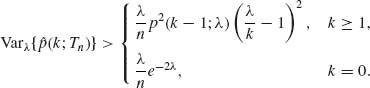
Strict inequality holds for all values of λ, 0 < λ < ∞, since the distribution of ![]() (k;Tn) is not of the exponential type, although the distribution of Tn is Poisson. The Poisson family satisfies all the conditions of Joshi (1976) and therefore since the distribution of
(k;Tn) is not of the exponential type, although the distribution of Tn is Poisson. The Poisson family satisfies all the conditions of Joshi (1976) and therefore since the distribution of ![]() (k;Tn) is not of the exponential type, the inequality is strict. Note that V{
(k;Tn) is not of the exponential type, the inequality is strict. Note that V{![]() (k;Tn} =
(k;Tn} = ![]() . We can compute this variance numerically.
. We can compute this variance numerically. ![]()
Example 5.7. Consider again the estimation problem of Examples 5.4 and 5.5, with k = 0. The MVUE of ω (λ) = e– λ is ![]() (Tn) =
(Tn) = ![]() . The variance of
. The variance of ![]() (Tn) can be obtained by considering the probability generating function of Tn ∼ P(nλ) at t =
(Tn) can be obtained by considering the probability generating function of Tn ∼ P(nλ) at t = ![]() . We thus obtain
. We thus obtain
![]()
Since ω(λ) is an analytic function, we can bound the variance of ![]() (Tn) from below by using BLB of order k = 2 (see (5.2.15)). We obtain,
(Tn) from below by using BLB of order k = 2 (see (5.2.15)). We obtain, ![]() . Hence, the lower bound for k = 2 is
. Hence, the lower bound for k = 2 is
![]()
This lower bound is larger than the Cramér – Rao lower bound for all 0 < λ < ∞. ![]()
Example 5.8. Let (X1, Y1), …, (Xn, Yn) be i.i.d. vectors having a common bivariate normal distribution ![]() . The complete sufficient statistic for this family of bivariate normal distributions is T1(X, Y) =
. The complete sufficient statistic for this family of bivariate normal distributions is T1(X, Y) = ![]() and T2(X, Y) =
and T2(X, Y) = ![]() . We wish to estimate the coefficient of correlation ρ.
. We wish to estimate the coefficient of correlation ρ.
An unbiased estimator of ρ is given by ![]() . Indeed
. Indeed
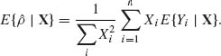
But E{Yi| X} = ρ Xi for all i = 1, …, n. Hence, E{![]() | X} = ρ w.p.1. The unbiased estimator is, however, not an MVUE. Indeed,
| X} = ρ w.p.1. The unbiased estimator is, however, not an MVUE. Indeed, ![]() is not a function of (T1(X, Y), T2(X, Y)). The MVUE can be obtained, according to the Rao – Blackwell Theorem by determining the conditional expectation E{
is not a function of (T1(X, Y), T2(X, Y)). The MVUE can be obtained, according to the Rao – Blackwell Theorem by determining the conditional expectation E{![]() | T1, T2}.
| T1, T2}.
The variance of ![]() is
is
![]()
The Fisher information matrix in the present case is
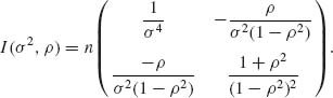
The inverse of the Fisher information matrix is
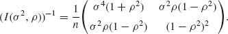
The lower bound on the variances of unbiased estimators of ρ is, therefore, (1 – ρ2)2/n. The ratio of the lower bound of the variance of ![]() to the actual variance is
to the actual variance is ![]() for large n. Thus,
for large n. Thus, ![]() is a good unbiased estimator only if ρ2 is close to zero.
is a good unbiased estimator only if ρ2 is close to zero. ![]()
Example 5.9.
![]()
The sample minimum X(1) is a complete sufficient statistic. X(1) is distributed like θ + G(n, 1). Hence, E{X(1)} = ![]() and the MVUE of θ is
and the MVUE of θ is ![]() (X(1)) =
(X(1)) = ![]() . The variance of this estimator is
. The variance of this estimator is
![]()
In the present case, the Fisher information I(θ) does not exist. We derive now the modified Chapman – Robbins lower bound for the variance of an unbiased estimator of θ. Notice first that W![]() (X(1);θ) = I{X(1) ≥
(X(1);θ) = I{X(1) ≥ ![]() } en(
} en(![]() – θ), where T = X(1), for all
– θ), where T = X(1), for all ![]() ≥ θ. It is then easy to prove that
≥ θ. It is then easy to prove that
![]()
Accordingly,
![]()
The function x2/(enx – 1) assumes a unique maximum over (0, ∞) at the root of the equation enx}(2 – nx) = 2. This root is approximately x0 = ![]() . This approximation yields
. This approximation yields
![]()
![]()
However,
![]()
![]()
Example 5.10. Let X1, …, Xn be i.i.d. random variables having the normal distribution N(θ, σ2) and Y1, …, Yn i.i.d. random variables having the normal distribution N(γ θ2, σ2), where -∞ < θ, γ < ∞, and 0 < σ < ∞. The vector X = (X1, …, Xn)′ is independent of Y = (Y1, …, Yn)′. A m.s.s. is (![]() n,
n, ![]() n, Qn), where
n, Qn), where ![]() n =
n = ![]() , and
, and ![]() . The Fisher information matrix can be obtained from the likelihood function
. The Fisher information matrix can be obtained from the likelihood function
![]()
The covariance matrix of the score functions is
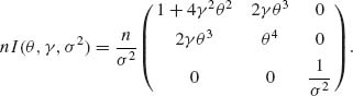
Thus,
![]()
Consider the reparametrization g1(θ, γ, σ) = θ, g2(θ, γ, σ2) = γ θ2 and g3(θ, γ, σ) = σ2. The UMVU estimator is ![]() = (
= (![]() n,
n, ![]() n, Qn/2(n – 1)). The variance covariance matrix of
n, Qn/2(n – 1)). The variance covariance matrix of ![]() is
is
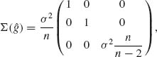
and
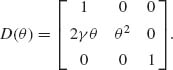
Thus, ![]() g =
g = ![]() . The efficiency coefficient is
. The efficiency coefficient is ![]() .
. ![]()
Example 5.11. Let (X1, Y1), …, (Xn, Yn) be a sample of n i.i.d. vectors having a joint bivariate normal distribution
![]()
where -∞ < μ < ∞, 0 < τ < ∞, 0 < σ < ∞, and – 1 < ρ < 1. Assume that σ2, τ2, and ρ are known. The problem is to estimate the common mean μ. We develop the formula of the BLUE of μ. In the present case,
![]()
and
![]()
The BLUE of the common mean μ is according to (5.3.3)
![]()
where ![]() n and
n and ![]() n are the sample means and
n are the sample means and
![]()
Since ![]() is known,
is known, ![]() is UMVU estimator.
is UMVU estimator. ![]()
Example 5.12. Let X1, …, Xn be i.i.d. Weibull variables, i.e., X∼ G1/β(λ, 1), where 0 < λ, β < ∞. Both λ and β are unknown. The m.s.s. is (X(1), …, X(n)). Let Yi = log Xi, i = 1, …, n, and Y(i) = log X(i). Obviously, Y(1) ≤ Y(2) ≤ … ≤ Y(n). We obtain the linear model
![]()
where μ = ![]() log λ and σ =
log λ and σ = ![]() ; G(i) is the ith order statistic of n i.i.d. variables distributed like G(1, 1). BLUEs of μ and σ are given by (5.4.16), where α is the vector of E{log G(i)} and V is the covariance matrix of log G(i).
; G(i) is the ith order statistic of n i.i.d. variables distributed like G(1, 1). BLUEs of μ and σ are given by (5.4.16), where α is the vector of E{log G(i)} and V is the covariance matrix of log G(i).
The p.d.f. of G(i) is
![]()
0 ≤ x ≤ ∞. Hence,

The integral on the RHS is proportional to the expected value of the extreme value distribution. Thus,

where γ = 0.577216… is the Euler constant. The values of αi can be determined numerically for any n and i = 1, …, n. Similar calculations yield formulae for the elements of the covariance matrix V. The point is that, from the obtained formulae of αi and Vij, we can determine the estimates only numerically. Moreover, the matrix V is of order n × n. Thus, if the sample involves a few hundreds observation the numerical inversion of V becomes difficult, if at all possible. ![]()
Example 5.13. Consider the multiple regression problem with p = 3, σ2 = 1, for which the normal equations are
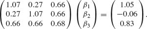
By employing the orthogonal (Helmert) transformation
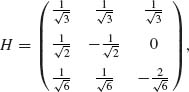
we obtain that
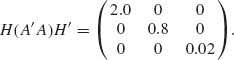
That is, the eigenvalues of A′A are λ1 = 2, λ2 = 0.8 and λ3 = 0.02. The LSEs of β are ![]() 1 = -4.58625,
1 = -4.58625, ![]() 2 = -5.97375, and
2 = -5.97375, and ![]() 3 = 11.47. The variance covariance matrix of the LSE is
3 = 11.47. The variance covariance matrix of the LSE is
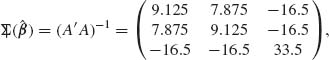
having a trace E{L2(0)} = 51.75 = ![]() . In order to illustrate numerically the effect of the ridge regression, assume that the true value of β is (1.5, -6.5, 0.5). Let γ = Hβ. The numerical value of γ is (-2.59809, 5.65685, -2.44949). According to (5.4.4), we can write the sum of the MSEs of the components of
. In order to illustrate numerically the effect of the ridge regression, assume that the true value of β is (1.5, -6.5, 0.5). Let γ = Hβ. The numerical value of γ is (-2.59809, 5.65685, -2.44949). According to (5.4.4), we can write the sum of the MSEs of the components of ![]() (k) by
(k) by
![]()
The estimate of k0 is ![]() = 0.249. In the following table, we provide some numerical results.
= 0.249. In the following table, we provide some numerical results.
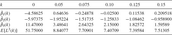
We see that the minimal E{L2(k)} is minimized for k0 around 0.125. At this value of k, ![]() (k) is substantially different from the LSE
(k) is substantially different from the LSE ![]() (0).
(0). ![]()
Example 5.14.
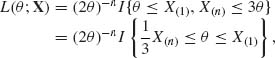
where X(1) = min {Xi} and X(n) = max {Xi}. The m.s.s. is (X(1), Xn. We note that according to the present model X(n) ≤ 3X(1). If this inequality is not satisfied then the model is incompatible with the data. It is easy to check that the MLE of θ is ![]() =
= ![]() . The MLE is not a sufficient statistic.
. The MLE is not a sufficient statistic.
![]()
Note that this likelihood function assumes a constant value 1 over the θ interval [X(n) – 1, X(1)]. Accordingly, any value of θ in this interval is an MLE. In the present case, the MLE is not unique. ![]()
Example 5.15. Let X1, …, Xn be i.i.d. random variables having a common Laplace (double–exponential) distribution with p.d.f.
![]()
-∞ < μ < ∞, 0 < β < ∞.
A m.s.s. in the present case is the order statistic X(1) ≤ … ≤ X(n). The likelihood function of (μ, β), given T = (X(1), …, X(n)), is
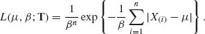
The value of μ which minimizes ![]() is the sample median Me. Hence,
is the sample median Me. Hence,
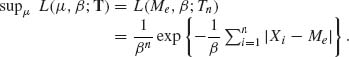
Finally, by differentiating log L(Me, β;T) with respect to β, we find that the value of β that maximizes L(Me, β;T) is
![]()
In the present case, the sample median Me and the sample mean absolute deviation from Me are the MLEs of μ and β, respectively. The MLE is not a sufficient statistic. ![]()
Example 5.16. Consider the normal case in which X1, …, Xn are i.i.d. random variables distributed like N(μ, σ2); -∞ < μ < ∞, 0 < σ2 < ∞. Both parameters are unknown. The m.s.s. is (![]() , Q), where
, Q), where ![]() =
= ![]() and
and ![]() . The likelihood function can be written as
. The likelihood function can be written as
![]()
Whatever the value of σ2 is, the likelihood function is maximized by ![]() =
= ![]() . It is easy to verify that the value of σ2 maximizing (5.5.9) is σ2 = Q/n.
. It is easy to verify that the value of σ2 maximizing (5.5.9) is σ2 = Q/n.
The normal distributions under consideration can be written as a two–parameter exponential type, with p.d.f.s
![]()
where
![]()
and ![]() . Differentiating the log–likelihood partially with respect to
. Differentiating the log–likelihood partially with respect to ![]() 1 and
1 and ![]() 2, we obtain that the MLEs of these (natural) parameters should satisfy the system of equations
2, we obtain that the MLEs of these (natural) parameters should satisfy the system of equations
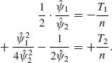
We note that T1/n = ![]() and T2/n =
and T2/n = ![]() 2 +
2 + ![]() 2 where
2 where ![]() =
= ![]() and
and ![]() 2 = Q/n are the MLEs of μ and σ2, respectively. Substituting of μ and σ2 + μ2, we obtain
2 = Q/n are the MLEs of μ and σ2, respectively. Substituting of μ and σ2 + μ2, we obtain ![]() 1 =
1 = ![]() /
/![]() 2,
2, ![]() 2 = -1/2
2 = -1/2![]() 2. In other words, the relationship between the MLEs
2. In other words, the relationship between the MLEs ![]() 1 and
1 and ![]() 2 to the MLEs
2 to the MLEs ![]() and
and ![]() 2 is exactly like that of
2 is exactly like that of ![]() 1 and
1 and ![]() 2 to μ and σ2.
2 to μ and σ2. ![]()
Example 5.17. Consider again the model of Example 5.9. Differentiating the log–likelihood
![]()
with respect to the parameters, we obtain the equations
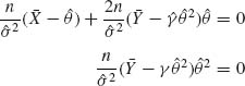
and
![]()
The unique solution of these equations is
![]()
and
![]()
It is interesting to realize that E{![]() } does not exist, and obviously
} does not exist, and obviously ![]() does not have a finite variance. By the delta method one can find the asymptotic mean and variance of
does not have a finite variance. By the delta method one can find the asymptotic mean and variance of ![]() .
. ![]()
Example 5.18. Let X1, …, Xn be i.i.d. random variables having a log–normal distribution LN(μ, σ2). The expected value of X and its variance are
![]()
and
![]()
We have previously shown that the MLEs of μ and σ2 are ![]() =
= ![]() and
and ![]() , where Yi = log Xi, i = 1, …, n. Thus, the MLEs of ξ and D2 are
, where Yi = log Xi, i = 1, …, n. Thus, the MLEs of ξ and D2 are
![]()
and
![]()
![]()
Example 5.19. Let X1, X2, …, Xn be i.i.d. random variables having a normal distribution N(μ, σ2), – ∞ < μ < ∞, 0 < σ2 < ∞. The MLEs of μ and σ2 are ![]() =
= ![]() n and
n and ![]() 2 =
2 = ![]() , where Q =
, where Q = ![]() . By the invariance principle, the MLE of θ =
. By the invariance principle, the MLE of θ = ![]() is
is ![]() .
. ![]()
Example 5.20. Consider the Weibull distributions, G1/β(λ, 1), where 0 < λ, β < ∞ are unknown. The likelihood function of (λ, β) is
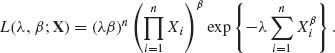
Note that the likelihood is equal to the joint p.d.f. of X multiplied by ![]() , which is positive with probability one. To obtain the MLEs of λ and β, we differentiate the log–likelihood partially with respect to these variables and set the derivatives equal to zero. We obtain the system of equations:
, which is positive with probability one. To obtain the MLEs of λ and β, we differentiate the log–likelihood partially with respect to these variables and set the derivatives equal to zero. We obtain the system of equations:
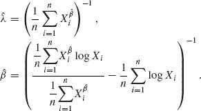
We show now that ![]() is always positive and that a unique solution exists. Let x = (x1, …, xn), where 0 < xi < ∞, i = 1, …, n, and let F(β;x) =
is always positive and that a unique solution exists. Let x = (x1, …, xn), where 0 < xi < ∞, i = 1, …, n, and let F(β;x) =![]() . Note that, for every x,
. Note that, for every x,
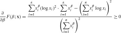
with a strict inequality if the xi values are not all the same. Indeed, if ωi = ![]() and
and ![]() then
then ![]() . Hence, F(β;x) is strictly increasing in β, with probability one. Furthermore,
. Hence, F(β;x) is strictly increasing in β, with probability one. Furthermore, ![]() and
and ![]() . Thus, the RHS of the β–equation is positive, decreasing function of β, approaching ∞ as β → 0 and approaching (log x(n) –
. Thus, the RHS of the β–equation is positive, decreasing function of β, approaching ∞ as β → 0 and approaching (log x(n) – ![]() as β → ∞. This proves that the solution
as β → ∞. This proves that the solution ![]() is unique.
is unique.
The solution for β can be obtained iteratively from the recursive equation
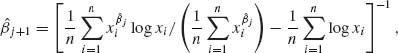
starting with ![]() 0 = 1.
0 = 1. ![]()
Example 5.21. The present example was given by Stein (1962) in order to illustrate a possible anomalous property of the MLE.
Let ![]() be a scale–parameter family of distributions, with p.d.f.
be a scale–parameter family of distributions, with p.d.f.
![]()
where
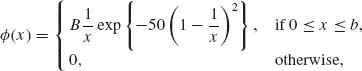
where
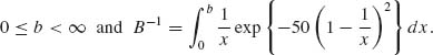
Note that 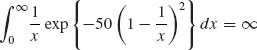 . Accordingly, we choose b sufficiently large so that
 ![]() . The likelihood function of θ corresponding to one observation is thus
. The likelihood function of θ corresponding to one observation is thus

The MLE of θ is ![]() = X. However, according to the construction of
= X. However, according to the construction of ![]() (x),
(x),
![]()
The MLE here is a bad estimator for all θ. ![]()
Example 5.22. Another source for anomality of the MLE is in the effect of nuisance parameters. A very well–known example of the bad effect of nuisance parameters is due to Neyman and Scott (1948). Their example is presented here.
Let (X1, Y1), …, (Xn, Yn) be n i.i.d. random vectors having the distributions N(μi12, σ2I2), i = 1, …, n. In other words, each pair (Xi, Yi) can be considered as representing two independent random variables having a normal distribution with mean μi and variance σ2. The variance is common to all the vectors. We note that Di = Xi – Yi ∼ N(0, 2σ2) for all i = 1, …, n. Hence, ![]() is an unbiased estimator of σ2. The variance of
is an unbiased estimator of σ2. The variance of ![]() is
is ![]() . Thus,
. Thus, ![]() approaches the value of σ2 with probability 1 for all (μi, σ). We turn now to the MLE of σ2. The parameter space is Θ = {μ1, …, μn, σ2: – ∞ < μ i < ∞, i = 1, …, n; 0 < σ2 < ∞ }. We have to determine a point (μ1, …, μn, σ2) that maximizes the likelihood function
approaches the value of σ2 with probability 1 for all (μi, σ). We turn now to the MLE of σ2. The parameter space is Θ = {μ1, …, μn, σ2: – ∞ < μ i < ∞, i = 1, …, n; 0 < σ2 < ∞ }. We have to determine a point (μ1, …, μn, σ2) that maximizes the likelihood function

We note that (xi – μi)2 + (yi – μi)2 is minimized by ![]() i = (xi + yi)/2. Thus,
i = (xi + yi)/2. Thus,
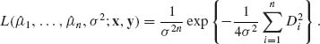
The value of σ2 that maximizes the likelihood is ![]() . Note that Eθ {
. Note that Eθ {![]() 2} = σ2/2 and that by the strong law of large numbers,
2} = σ2/2 and that by the strong law of large numbers, ![]() 2 → σ2/2 with probability one for each σ2.
2 → σ2/2 with probability one for each σ2.
Thus, the more information we have on σ2 (the larger the sample is) the worse the MLE becomes. It is interesting that if we do not use all the information available then the MLE may become a reasonable estimator. Note that at each given value of σ2, Mi = (Xi + Yi)/2 is a sufficient statistic for μi. Accordingly, the conditional distribution of (X, Y) given M = (M1, …, Mn)′ is independent of μ. If we consider the semi–likelihood function, which is proportional to the conditional p.d.f. of (X, Y), given M and σ2, then the value of σ2 that maximizes this semi–likelihood function coincides with the unbiased estimator ![]() .
. ![]()
Example 5.23. Consider the standard logistic tolerance distribution, i.e.,
![]()
The corresponding p.d.f. is
![]()
The corresponding function G(z;![]() ) given by (5.6.10) is
) given by (5.6.10) is
![]()
The logit, F−1(z), is given by
![]()
Let ![]() i be the observed proportion of response at dosage xi. Define
i be the observed proportion of response at dosage xi. Define ![]() i =
i = ![]() , if 0 <
, if 0 < ![]() i < 1.
i < 1.
According to the model
![]()
We, therefore, fit by least squares the line
![]()
to obtain the initial estimates of α and β. After that we use the iterative procedure (5.6.12) to correct the initial estimates. For example suppose that the dosages (log dilution) are x1 = -2.5, x2 = -2.25, x3 = -2, x4 = -1.75, and x5 = -1.5. At each dosage a sample of size n = 20 is observed, and the results are
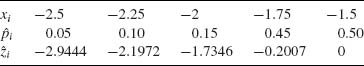
Least–squares fitting of the regression line ![]() i =
i = ![]() +
+ ![]() xi yields the initial estimates
xi yields the initial estimates ![]() = 4.893 and
= 4.893 and ![]() = 3.154. Since G′(z;
= 3.154. Since G′(z;![]() ) = -f(z), we define the weights
) = -f(z), we define the weights
![]()
and
![]()
We solve then equations (5.6.12) to obtain the corrections to the initial estimates. The first five iterations gave the following results:
| j | ||
| 0 | 4.89286 | 3.15412 |
| 1 | 4.93512 | 3.16438 |
| 2 | 4.93547 | 3.16404 |
| 3 | 4.93547 | 3.16404 |
| 4 | 4.93547 | 3.16404 |
![]()
Example 5.24. X1, …, Xn are i.i.d. random variables distributed like N(μ, σ2), where -∞ < μ < ∞, 0 < σ < ∞. The group ![]() considered is that of the real–affine transformations. A m.s.s. is (
considered is that of the real–affine transformations. A m.s.s. is (![]() , Q), where
, Q), where ![]() =
= ![]() and Q =
and Q = ![]() . If [α, β] is an element of
. If [α, β] is an element of ![]() then
then
![]()
and
![]()
If ![]() (
(![]() , Q) is an equivariant estimator of μ then
, Q) is an equivariant estimator of μ then
![]()
for all [α, β] ![]()
![]() . Similarly, every equivariant estimator of σ2 should satisfy the relationship
. Similarly, every equivariant estimator of σ2 should satisfy the relationship
![]()
for all [α, β] ![]()
![]() . The m.s.s. (
. The m.s.s. (![]() , Q) is reduced by the transformation [-
, Q) is reduced by the transformation [-![]() , 1] to (0, Q). This transformation is a maximal invariant reduction of (
, 1] to (0, Q). This transformation is a maximal invariant reduction of (![]() , Q) with respect to the subgroup of translations
, Q) with respect to the subgroup of translations ![]() 1 = {[α, 1], -∞ < α < ∞ }. The difference D(
1 = {[α, 1], -∞ < α < ∞ }. The difference D(![]() , Q) =
, Q) = ![]() (
(![]() , Q)-
, Q)-![]() is translation invariant, i.e., [α, 1]D(
is translation invariant, i.e., [α, 1]D(![]() , Q) = D(
, Q) = D(![]() , Q) for all [α, 1]
, Q) for all [α, 1] ![]()
![]() 1. Hence, D(
1. Hence, D(![]() , Q) is a function of the maximal invariant with respect to
, Q) is a function of the maximal invariant with respect to ![]() 1. Accordingly, every equivariant estimator can be expressed as
1. Accordingly, every equivariant estimator can be expressed as
![]()
where f(Q) is a statistic depending only on Q. Similarly, we can show that every equivariant estimator of σ2 should be of the form
![]()
where λ is a positive constant. We can also determine the equivariant estimators of μ and σ2 having the minimal MSE. We apply the result that ![]() and Q are independent. The MSE of
and Q are independent. The MSE of ![]() + f(Q) for any statistic f(Q) is
+ f(Q) for any statistic f(Q) is
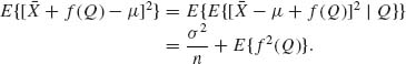
Hence, the MSE is minimized, by choosing f(Q) = 0. Accordingly, the sample mean, ![]() is the minimal MSE equivariant estimator of μ. Similarly, one can verify that the equivariant estimator of σ2, which has the minimal MSE, is
is the minimal MSE equivariant estimator of μ. Similarly, one can verify that the equivariant estimator of σ2, which has the minimal MSE, is ![]() 2 = Q/(n + 1). Note that this estimator is biased. The UMVU estimator is Q/(n – 1) and the MLE is Q/n.
2 = Q/(n + 1). Note that this estimator is biased. The UMVU estimator is Q/(n – 1) and the MLE is Q/n. ![]()
Example 5.25. Let X1, …, Xn be i.i.d. random variables having a common N(μ, ![]() ) distribution. Let Y1, …, Yn be i.i.d. random variables distributed as N(μ,
) distribution. Let Y1, …, Yn be i.i.d. random variables distributed as N(μ, ![]() ). The X and the Y vectors are independent. The two distributions have a common mean μ, -∞ < μ < ∞, and possibly different variances. The variance ratio ρ =
). The X and the Y vectors are independent. The two distributions have a common mean μ, -∞ < μ < ∞, and possibly different variances. The variance ratio ρ = ![]() is unknown. A m.s.s. is (
is unknown. A m.s.s. is (![]() , Q(X),
, Q(X), ![]() , Q(Y)), where
, Q(Y)), where ![]() and
and ![]() are the sample means and Q(X) and Q(Y) are the sample sums of squares of deviations around the means.
are the sample means and Q(X) and Q(Y) are the sample sums of squares of deviations around the means. ![]() , Q(X),
, Q(X), ![]() , and Q(Y) are mutually independent. Consider the group
, and Q(Y) are mutually independent. Consider the group ![]() of affine transformations
of affine transformations ![]() = {[α, β]: -∞ < α < ∞, -∞ < β < ∞ }. A maximal invariant statistic is V =
= {[α, β]: -∞ < α < ∞, -∞ < β < ∞ }. A maximal invariant statistic is V = ![]() . Let W = (
. Let W = (![]() ,
, ![]() -
-![]() ). The vector (W, V) is also a m.s.s. Note that
). The vector (W, V) is also a m.s.s. Note that
![]()
for all [α, β] ![]()
![]() . Hence, if
. Hence, if ![]() (W, V) is an equivariant estimator of the common mean μ it should be of the form
(W, V) is an equivariant estimator of the common mean μ it should be of the form
![]()
where ![]() (V) is a function of the maximal invariant statistic V. Indeed,
(V) is a function of the maximal invariant statistic V. Indeed, ![]() ≠
≠ ![]() with probability one, and (
with probability one, and (![]() (W, V) –
(W, V) – ![]() )/(
)/(![]() –
– ![]() ) is an invariant statistic, with respect to
) is an invariant statistic, with respect to ![]() . We derive now the MSE of
. We derive now the MSE of ![]() (W, V). We prove first that every such equivariant estimator is unbiased. Indeed, for every θ = (μ,
(W, V). We prove first that every such equivariant estimator is unbiased. Indeed, for every θ = (μ, ![]() , ρ)
, ρ)
![]()
Moreover, by Basu’s Theorem (3.6.1), V is independent of (![]() ,
, ![]() ). Hence,
). Hence,
![]()
with probability one, since the distribution of ![]() –
– ![]() is symmetric around zero. This implies the unbiasedness of
is symmetric around zero. This implies the unbiasedness of ![]() (W, V). The variance of this estimator is
(W, V). The variance of this estimator is
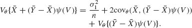
Since Eθ {(![]() –
– ![]() )
)![]() (V)} = 0, we obtain that
(V)} = 0, we obtain that
![]()
The distribution of ![]() – μ depends only on
– μ depends only on ![]() . The maximal invariant statistic V is independent of μ and
. The maximal invariant statistic V is independent of μ and ![]() . It follows from Basu’s Theorem that (
. It follows from Basu’s Theorem that (![]() – μ) and
– μ) and ![]() (V) are independent. Moreover, the conditional distribution of
(V) are independent. Moreover, the conditional distribution of ![]() – μ given
– μ given ![]() –
– ![]() is the normal distribution
is the normal distribution ![]() . Thus,
. Thus,
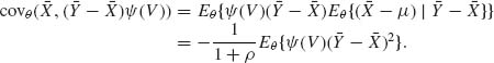
The conditional distribution of (![]() -
-![]() )2 given V is the gamma distribution G(λ, ν) with
)2 given V is the gamma distribution G(λ, ν) with
![]()
where Z1 = Q(X)/(![]() –
– ![]() )2 and Z2 = Q(Y)/(
)2 and Z2 = Q(Y)/(![]() –
– ![]() )2. We thus obtain the expression
)2. We thus obtain the expression
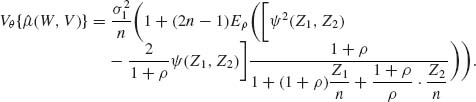
We see that in the present example the variance divided by ![]() /n depends not only on the particular function
/n depends not only on the particular function ![]() (Z1, Z2) but also on the (nuisance) parameter ρ =
(Z1, Z2) but also on the (nuisance) parameter ρ = ![]() . This is due to the fact that ρ is invariant with respect to
. This is due to the fact that ρ is invariant with respect to ![]() . Thus, if ρ is unknown there is no equivariant estimator having minimum variance for all θ values. There are several papers in which this problem is studied (Brown and Cohen, 1974; Cohen and Sackrowitz, 1974; Kubokawa, 1987; Zacks, 1970a).
. Thus, if ρ is unknown there is no equivariant estimator having minimum variance for all θ values. There are several papers in which this problem is studied (Brown and Cohen, 1974; Cohen and Sackrowitz, 1974; Kubokawa, 1987; Zacks, 1970a). ![]()
Example 5.26. Let X1, …, Xn be i.i.d. random variables having a common Weibull distribution G1/β(λ– β, 1), where 0 < λ, β < ∞. Note that the parametrization here is different from that of Example 5.20. The present parametrization yields the desired structural properties. The m.s.s. is the order statistic, T(X) = (X(1), …, X(n)), where X(1) ≤ … ≤ X(n). Let ![]() (T) and
(T) and ![]() (T) be the MLEs of λ and β, respectively. We obtain the values of these estimators as in Example 5.20, with proper modification of the likelihood function. Define the group of transformations
(T) be the MLEs of λ and β, respectively. We obtain the values of these estimators as in Example 5.20, with proper modification of the likelihood function. Define the group of transformations
![]()
where
![]()
Note that the distribution of [a, b]X is as that of aλ1/bG1/β b (1, 1) or as that of G1/β b((aλ1/b)-bβ, 1). Accordingly, if X→ [a, b]X then the parametric point (λ, β) is transformed to
![]()
It is easy to verify that
![]()
and
![]()
The reduction of the m.s.s. T by the transformation [![]() ,
, ![]() ]−1 yields the maximal invariant U(T)
]−1 yields the maximal invariant U(T)
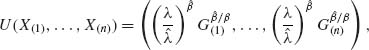
where G(1) ≤ … ≤ G(n) is the order statistic of n i.i.d. E(1) random variables. The distribution of U(T) does not depend on (λ, β). Thus, ![]() is distributed independently of (λ, β) and so is that of
is distributed independently of (λ, β) and so is that of ![]() /β.
/β.
Let ![]() = F(
= F(![]() ,
, ![]() , U(T)) and
, U(T)) and ![]() = G(
= G(![]() ,
, ![]() , U(T)) be equivariant estimators of λ and β respectively. According to the definition of equivariance
, U(T)) be equivariant estimators of λ and β respectively. According to the definition of equivariance
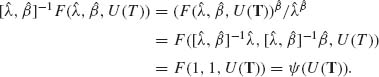
Accordingly, every equivariant estimator of λ is of the form
![]()
Similarly, every equivariant estimator β is of the form
![]()
Note that the relationship between the class of all equivariant estimators (![]() ,
, ![]() ) and the MLEs (
) and the MLEs (![]() ,
, ![]() ). In particular, if we choose
). In particular, if we choose ![]() (U(T)) = 1 w.p.l and H(U(T)) = 1 w.p.l we obtain that the MLEs
(U(T)) = 1 w.p.l and H(U(T)) = 1 w.p.l we obtain that the MLEs ![]() and
and ![]() are equivariant. This property also follows from the fact that the MLE of
are equivariant. This property also follows from the fact that the MLE of ![]() is
is ![]() for all [a, b] in
for all [a, b] in ![]() . We will consider now the problem of choosing the functions H(U(T)) and
. We will consider now the problem of choosing the functions H(U(T)) and ![]() (U(T)) to minimize the risk of the equivariant estimator. For this purpose we consider a quadratic loss function in the logarithms, i.e.,
(U(T)) to minimize the risk of the equivariant estimator. For this purpose we consider a quadratic loss function in the logarithms, i.e.,
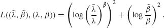
It is easy to check that this loss function is invariant with respect to ![]() . Furthermore, the risk function does not depend on (λ, β). We can, therefore, choose
. Furthermore, the risk function does not depend on (λ, β). We can, therefore, choose ![]() and H to minimize the risk. The conditional risk function, given U(T), when
and H to minimize the risk. The conditional risk function, given U(T), when ![]() (U(T)) =
(U(T)) = ![]() and H(U(T)) = H, is
and H(U(T)) = H, is
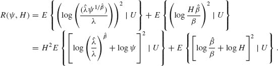
Since ![]() and
and ![]() are ancillary statistics, and since T is a complete sufficient statistic, we infer from Basu’s Theorem that
are ancillary statistics, and since T is a complete sufficient statistic, we infer from Basu’s Theorem that ![]() and
and ![]() are independent of U(T). Hence, the conditional expectations are equal to the total expectations. Partial differentiation with respect to H and
are independent of U(T). Hence, the conditional expectations are equal to the total expectations. Partial differentiation with respect to H and ![]() yields the system of equations:
yields the system of equations:
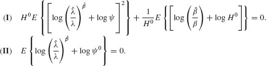
From equation (II), we immediately obtain the expression
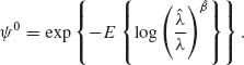
Substituting this ![]() 0 in (I), we obtain the equation
0 in (I), we obtain the equation

This equation can be solved numerically to obtain the optimal constant H0. Thus, by choosing the functions ![]() (U) and H(U) equal (with probability one) to the constants
(U) and H(U) equal (with probability one) to the constants ![]() 0 and H0, respectively, we obtain the minimum MSE equivariant estimators. We can estimate
0 and H0, respectively, we obtain the minimum MSE equivariant estimators. We can estimate ![]() 0 and H0 by simulation, using the special values of λ = 1 and β = 1.
0 and H0 by simulation, using the special values of λ = 1 and β = 1. ![]()
Example 5.27. As in Example 5.15, let X1, …, Xn be i.i.d random variables having a Laplace distribution with a location parameter μ and scale parameter β, where -∞ < μ < ∞ and 0 < β < ∞. The two moments of this distribution are
![]()
The sample moments are M1 = ![]() and M2 =
and M2 = ![]() . Accordingly, the MEEs of μ and β are
. Accordingly, the MEEs of μ and β are
![]()
where ![]() 2 = M2 –
2 = M2 – ![]() . It is interesting to compare these MEEs to the MLEs of μ and β that were derived in Example 5.15. The MLE of μ is the sample median Me, while the MEE of μ is the sample mean
. It is interesting to compare these MEEs to the MLEs of μ and β that were derived in Example 5.15. The MLE of μ is the sample median Me, while the MEE of μ is the sample mean ![]() . The MEE is an unbiased estimator of μ, with variance V{
. The MEE is an unbiased estimator of μ, with variance V{![]() } = 2β2/n. The median is also an unbiased estimator of μ. Indeed, let n = 2m + 1 then Me ∼ μ + β Y(m + 1), where Y(m + 1) is the (m + 1)st order statistic of a sample of n = 2m + 1 i.i.d. random variables having a standard Laplace distribution (μ = 0, β = 1). The p.d.f. of Y(m + 1) is
} = 2β2/n. The median is also an unbiased estimator of μ. Indeed, let n = 2m + 1 then Me ∼ μ + β Y(m + 1), where Y(m + 1) is the (m + 1)st order statistic of a sample of n = 2m + 1 i.i.d. random variables having a standard Laplace distribution (μ = 0, β = 1). The p.d.f. of Y(m + 1) is
![]()
where
![]()
and
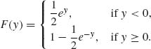
It is easy to verify that g(-y) = g(y) for all -∞ < y < ∞. Hence, E{Y(m + 1)} = 0 and E{Me} = μ. The variance of Me, for m≥ 1, is
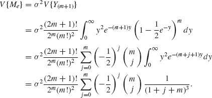
Thus, for β = 1, one obtains the following values for the variances of the estimators:

We see that the variance of Me in small samples is about half the variance of ![]() n. As will be shown in Section 5.10, as n → ∞, the ratio of the asymptotic variances approaches 1/2. It is also interesting to compare the expectations and MSE of the MLE and MEE of the scale parameter β.
n. As will be shown in Section 5.10, as n → ∞, the ratio of the asymptotic variances approaches 1/2. It is also interesting to compare the expectations and MSE of the MLE and MEE of the scale parameter β. ![]()
Example 5.28. Let X1, …, Xn be i.i.d. random variables having a common log–normal distribution LN(μ, σ2), -∞ < μ < ∞, and 0 < σ2 < ∞. Let Yi = log Xi, i = 1, …, n; ![]() n =
n = ![]() and
and ![]() .
. ![]() n and
n and ![]() are the MLEs of μ and σ2, respectively. We derive now the MEEs of μ and σ2. The first two moments of LN(μ, σ2) are
are the MLEs of μ and σ2, respectively. We derive now the MEEs of μ and σ2. The first two moments of LN(μ, σ2) are
![]()
Accordingly, the MEEs of μ and σ2 are
![]()
where M1 = ![]() n and M2 =
n and M2 = ![]() are the sample moments. Note that the MEEs
are the sample moments. Note that the MEEs ![]() and
and ![]() 2 are not functions of the minimal sufficient statistics
2 are not functions of the minimal sufficient statistics ![]() n and
n and ![]() 2, and therefore are expected to have larger MSEs than those of the MLEs.
2, and therefore are expected to have larger MSEs than those of the MLEs. ![]()
Example 5.29. In Example 5.20, we discussed the problem of determining the values of the MLEs of the parameters λ and β of the Weibull distribution, where X1, …, Xn are i.i.d. like G1/β(λ, 1) where 0 < β, λ < ∞. The MEEs are obtained in the following manner. According to Table 2.2, the first two moments of G1/β(λ, 1) are
![]()
Thus, we set the moment equations
![]()
Accordingly, the MEE ![]() is the root of the equation
is the root of the equation
![]()
The solution of this equation can be obtained numerically. After solving for ![]() , one obtains
, one obtains ![]() as follows:
as follows:
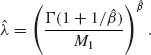
We illustrate this solution with the numbers in the sample of Example 5.14. In that sample, n = 50, ![]() = 46.6897, and
= 46.6897, and ![]() = 50.9335. Thus, M1 = .9338 and M2 = 1.0187. Equation (5.8.9) becomes
= 50.9335. Thus, M1 = .9338 and M2 = 1.0187. Equation (5.8.9) becomes
![]()
The solution should be in the neighborhood of β = 2, since 2 × 1.71195 = 3.4239 and ![]() = π = 3.14195…. In the following table, we approximate the solution:
= π = 3.14195…. In the following table, we approximate the solution:
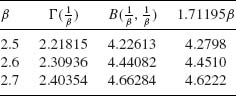
Accordingly, the MEE of β is approximately ![]() = 2.67 and that of λ is approximately
= 2.67 and that of λ is approximately ![]() = 0.877. The values of the MLE of β and λ, obtained in Example 5.20, are 1.875 and 0.839, respectively. The MLEs are closer to the true values, but are more difficult to obtain.
= 0.877. The values of the MLE of β and λ, obtained in Example 5.20, are 1.875 and 0.839, respectively. The MLEs are closer to the true values, but are more difficult to obtain. ![]()
Example 5.30.
The likelihood function of ρ is
![]()
where QX = ![]() . Note that the m.s.s. is T = (QX + QY, PXY). The maximal likelihood estimator of ρ is a real solution of the cubic equation
. Note that the m.s.s. is T = (QX + QY, PXY). The maximal likelihood estimator of ρ is a real solution of the cubic equation
![]()
where S = Qx + Qy. In the present example, the MEE is a very simple estimator. There are many different unbiased estimators of ρ. The MEE is one such unbiased estimator. Another one is
![]()
![]()
-∞ < θ, γ < ∞, 0 < σ2 < ∞. The MEE of σ2 is ![]() . Similarly, we find that the MEEs of θ and γ are
. Similarly, we find that the MEEs of θ and γ are
![]()
The MLEs are the same. ![]()
Example 5.31. Let X1, …, Xn be i.i.d. random variables having a common N(μ, σ2) distribution. The problem is to estimate the variance σ2. If μ = 0 then the minimum MSE equivariant estimator of σ2 is ![]() . On the other hand, if μ is unknown the minimum MSE equivariant estimator of σ2 is
. On the other hand, if μ is unknown the minimum MSE equivariant estimator of σ2 is ![]() , where
, where ![]() . One could suggest to test first the hypothesis H0: μ = 0, σ arbitrary, against H1: μ ≠ 0, σ arbitrary, at some level of significance α. If H0 is accepted the estimator is
. One could suggest to test first the hypothesis H0: μ = 0, σ arbitrary, against H1: μ ≠ 0, σ arbitrary, at some level of significance α. If H0 is accepted the estimator is ![]() , otherwise, it is
, otherwise, it is ![]() . Suppose that the preliminary test is the t–test. Thus, the estimator of σ2 assumes the form:
. Suppose that the preliminary test is the t–test. Thus, the estimator of σ2 assumes the form:
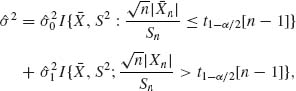
where ![]() is the sample variance. Note that this PTE is not translation invariant, since neither the t–test of H0 is translation invariant, nor is
is the sample variance. Note that this PTE is not translation invariant, since neither the t–test of H0 is translation invariant, nor is ![]() . The estimator σ2 may have smaller MSE values than those of
. The estimator σ2 may have smaller MSE values than those of ![]() or of
or of ![]() , on some intervals of (μ, σ2) values. Actually,
, on some intervals of (μ, σ2) values. Actually, ![]() 2 has smaller MSE than that of
2 has smaller MSE than that of ![]() for all (μ, σ2) if
for all (μ, σ2) if ![]() . This corresponds to (when n is large) a value of α approximately equal to α = 0.3173.
. This corresponds to (when n is large) a value of α approximately equal to α = 0.3173. ![]()
Example 5.32. Let X1, …, Xn be a sample of i.i.d. random variables from N(μ, ![]() ) and let Y1, …, Yn be a sample of i.i.d. random variables from N(μ,
) and let Y1, …, Yn be a sample of i.i.d. random variables from N(μ, ![]() ). The X and Y vectors are independent. The problem is to estimate the common mean μ. In Example 5.24, we studied the MSE of equivariant estimators of the common mean μ. In Chapter 8, we will discuss the problem of determining an optimal equivariant estimator of μ in a Bayesian framework. We present here a PTE of μ. Let ρ =
). The X and Y vectors are independent. The problem is to estimate the common mean μ. In Example 5.24, we studied the MSE of equivariant estimators of the common mean μ. In Chapter 8, we will discuss the problem of determining an optimal equivariant estimator of μ in a Bayesian framework. We present here a PTE of μ. Let ρ = ![]() . If ρ = 1 then the UMVU estimator of μ is
. If ρ = 1 then the UMVU estimator of μ is ![]() 1 = (
1 = (![]() +
+ ![]() )/2, where
)/2, where ![]() and
and ![]() are the sample means. When ρ is unknown then a reasonably good unbiased estimator of μ is
are the sample means. When ρ is unknown then a reasonably good unbiased estimator of μ is ![]() R = (
R = (![]() R +
R + ![]() )/(R + 1), where R =
)/(R + 1), where R = ![]() is the ratio of the sample variances
is the ratio of the sample variances ![]() to
to ![]() . A PTE of μ can be based on a preliminary test of H0: ρ = 1, μ, σ1, σ2 arbitrary against H1: ρ ≠ 1, μ, σ1, σ2 arbitrary. If we apply the F–test, we obtain the PTE
. A PTE of μ can be based on a preliminary test of H0: ρ = 1, μ, σ1, σ2 arbitrary against H1: ρ ≠ 1, μ, σ1, σ2 arbitrary. If we apply the F–test, we obtain the PTE
![]()
This estimator is unbiased, since ![]() and
and ![]() are independent of R. Furthermore,
are independent of R. Furthermore,
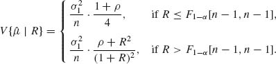
Hence, since E{![]() | R} = μ for all R, we obtain from the law of total variance that the variance of the PTE is
| R} = μ for all R, we obtain from the law of total variance that the variance of the PTE is
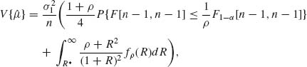
where R* = F1 – α[n – 1, n – 1], and fρ (R) is the p.d.f. of ρ F[n – 1, n – 1] at R. Closed formulae in cases of small n were given by Zacks (1966). ![]()