PART III: PROBLEMS
Section 2.2
2.2.1 Consider the binomial distribution with parameters n, θ, 0 < θ < 1.
Write an algorithm for the computation of b(j | n, θ) employing the recursive relationship
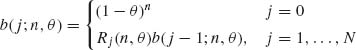
where Rj (n, θ) = b(j;n, θ)/b(j – 1; n, θ). Write the ratio Rj (n, θ) explicitly and find an expression for the mode of the distribution, i.e., ![]() = smallest nonnegative integer for which b(x0;n, θ) ≥ b(j; n, θ) for all j = 0, …, n.
= smallest nonnegative integer for which b(x0;n, θ) ≥ b(j; n, θ) for all j = 0, …, n.
2.2.2 Prove formula (2.2.2).
2.2.3 Determine the median of the binomial distribution with n = 15 and θ = .75.
2.2.4 Prove that when n → ∞, θ → 0, but nθ → λ, 0 < λ < ∞, then
![]()
where p(i; λ) is the p.d.f. of the Poisson distribution.
2.2.5 Establish formula (2.2.7).
2.2.6 Let X have the Pascal distribution with parameters ν (fixed positive integer) and θ, 0 < θ < 1. Employ the relationship between the Pascal distribution and the negative–binomial distribution to show that the median of X is ν + n.5, where n.5 = least nonnegative integer n such that Iθ (ν, n + 1) ≥ .5. [This formula of the median is useful for writing a computer program and utilizing the computer’s library subroutine function that computes Iθ (a, b).]
2.2.7 Apply formula (2.2.4) to prove the binomial c.d.f. B(j; n, θ) is a decreasing function of θ, for each j = 0, 1, …, n.
2.2.8 Apply formula (2.2.12) to prove that the c.d.f. of the negative–binomial distribution, NB(ψ, ν), is strictly decreasing in ψ, for a fixed ν, for each j = 0, 1, ….
2.2.9 Let X ∼ B(105, .0003). Apply the Poisson approximation to compute P{20 < X < 40}.
Section 2.3
2.3.1 Let U be a random variable having a rectangular distribution R(0, 1). Let β1(p | a, b), 0 < p < 1, 0 < a, b < ∞ denote the pth quantile of the β (a, b) distribution. What is the distribution of Y = β1(U; a, b)?
2.3.2 Let X have a gamma distribution ![]() , and k be a positive integer. Let
, and k be a positive integer. Let ![]() denote the pth quantile of the chi–squared distribution with ν degrees of freedom. Express the pth quantile of
denote the pth quantile of the chi–squared distribution with ν degrees of freedom. Express the pth quantile of ![]() in terms of the corresponding quantiles of the chi–squared distributions.
in terms of the corresponding quantiles of the chi–squared distributions.
2.3.3 Let Y have the extreme value distribution (2.3.19). Derive formulae for the pth quantile of Y and for its interquartile range.
2.3.4 Let n(x;ξ, σ2) denote the p.d.f. of the normal distribution N(ξ, σ2). Prove that
![]()
for all (ξ, σ2); -∞ < ξ < ∞, 0 < σ2 < ∞.
2.3.5 Let X have the binomial distribution with n = 105 and θ = 10-3. For large values of λ (λ > 30), the N(λ, λ) distribution provides a good approximation to the c.d.f. of the Poisson distribution P(λ). Apply this property to approximate the probability P{90 < X < 110}.
2.3.6 Let X have an exponential distribution E(λ), 0 < λ < ∞. Prove that for all t > 0, E{exp{–tX}} ≥ exp{-t/λ}.
2.3.7 Let x ∼ R(0, 1) and Y = – log X.
2.3.8 Determine the first four cumulants of the gamma distribution G(λ, ν), 0 < λ, ν < ∞. What are the coefficients of skewness and kurtosis?
2.3.9 Derive the coefficients of skewness and kurtosis of the log–normal distribution LN(μ, σ).
2.3.10 Derive the coefficients of skewness and kurtosis of the beta distribution β (p, q).
Section 2.4
2.4.1 Let X and Y be independent random variables and P{Y ≥ 0} = 1. Assume also that E{|X|} < ∞ and ![]() . Apply the Jensen inequality and the law of the iterated expectation to prove that
. Apply the Jensen inequality and the law of the iterated expectation to prove that
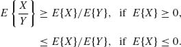
2.4.2 Prove that if X and Y are positive random variables and E{Y | X} = bX, 0 < b < ∞, then
2.4.3 Let X and Y be independent random variables. Show that cov(X + Y, X – Y) = 0 if and only if V{X} = V{Y}.
2.4.4 Let X and Y be independent random variables having a common normal distribution N(0, 1). Find the distribution of R = X/Y. Does E{R} exist?
2.4.5 Let X and Y be independent random variables having a common log–normal distribution LN(μ, σ2), i.e., log X ∼ log Y ∼ N(μ, σ2).
2.4.6 Let X have a binomial distribution B(n, θ) and let U∼ R(0, 1) independently of X and Y = X + U.
2.4.7 Suppose that the conditional distribution of X given θ is the binomial B(n, θ). Furthermore, assume that θ is a random variable having a beta distribution β (p, q).
2.4.8 Prove that if the conditional distribution of X given λ is the Poisson P(λ), and if λ has the gamma distribution as ![]() , then the marginal distribution of X is the negative–binomial
, then the marginal distribution of X is the negative–binomial ![]() .
.
2.4.9 Let X and Y be independent random variables having a common exponential distribution, E(λ). Let U = X + Y and W = X – Y.
![]()
2.4.10 Let X have a standard normal distribution as N(0, 1). Let Y = Φ(X). Show that the correlation between X and Y is ρ = (3/π)1/2. [Although Y is completely determined by X, i.e., V{Y | X} = 0 for all X, the correlation ρ is less than 1. This is due to the fact that Y is a nonlinear function of X.]
2.4.11 Let X and Y be independent standard normal random variables. What is the distribution of the distance of (X, Y) from the origin?
2.4.12 Let X have a χ2[ν] distribution. Let Y = δ X, where 1 < δ ∞. Express the m.g.f. of Y as a weighted average of the m.g.f.s of χ2[ν + 2j], j = 0, 1, …, with weights given by ωj = P[J = j], where ![]() . [The distribution of Y = δ X can be considered as an infinite mixture of χ2[ν + 2J] distributions, where J is a random variable having a negative–binomial distribution.]
. [The distribution of Y = δ X can be considered as an infinite mixture of χ2[ν + 2J] distributions, where J is a random variable having a negative–binomial distribution.]
2.4.13 Let X and Y be independent random variables; x ∼ χ2[ν1] and Y∼ δ χ2[ν2], 1 < δ ∞. Use the result of the previous exercise to prove that X + Y∼ χ2[ν1 +ν2 + 2J], where ![]() . [Hint: Multiply the m.g.f.s of X and Y or consider the conditional distribution of X + Y given J, where J is independent of X and Y | J∼ χ2[ν2 + 2J], J ∼ NB
. [Hint: Multiply the m.g.f.s of X and Y or consider the conditional distribution of X + Y given J, where J is independent of X and Y | J∼ χ2[ν2 + 2J], J ∼ NB![]() .]
.]
2.4.14 Let X1, …, Xn be identically distributed independent random variables having a continuous distribution F symmetric around μ. Let M(X1, …, Xn) and Q(X1, …, Xn) be two functions of X = (X1, …, Xn)′ satisfying:
then cov(M(X1, …, X_n), Q(X1, …, Xn)) = 0.
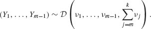
2.4.15 Let Y1, …, Yk-1 (k ≥ 3), Yi ≥ 0, ![]() , have a joint Dirichlet distribution
, have a joint Dirichlet distribution ![]() (ν1, ν2, …, νk), 0 < νi < ∞, i = 1, …, k.
(ν1, ν2, …, νk), 0 < νi < ∞, i = 1, …, k.

Section 2.5
2.5.1 Let X1, …, Xn be i.i.d. random variables. ![]() is the sample moment of order r. Assuming that all the required moments of the common distribution of Xi (i = 1, …, n) exist, find
is the sample moment of order r. Assuming that all the required moments of the common distribution of Xi (i = 1, …, n) exist, find
2.5.2 Let Uj, j = 0, ± 1, ± 2, …, be a sequence of independent random variables, such that E{Uj} = 0 and V{Uj} = σ2 for all j. Define the random variables Xt = β0 + β1Ut – 1 + β2Ut – 2 + … + βpUt – p + Ut, t = 0, 1, 2, …, where β0, …, βp are fixed constants. Derive
[The sequence {Xi} is called an autoregressive time series of order p. Notice that E{Xt}, V{Xt}, and cov(Xt, Xt+h) do not depend on t. Such a series is therefore called covariance stationary.]
2.5.3 Let X1, …, Xn be random variables represented by the model Xi = μi + ei (i = 1, …, n), where e1, …, en are independent random variables, E{ei} = 0 and V{ei} = σ2 for all i = 1, …, n. Furthermore, let μ1 be a constant and μi = μi – 1 + Ji (i = 1, 2, …, n), where J2, …, Jn are independent random variables, Ji ∼ B(1, p), i = 2, …, n. Let X = (X1, …, Xn)′. Determine
2.5.4 Let X1, …, Xn be i.i.d. random variables. Assume that all required moments exist. Find
Section 2.6
2.6.1 Let (X1, X2, X3) have the trinomial distribution with parameters n = 20, θ1 = .3, θ2 = .6, θ3 = .1.
2.6.2 Let (X1, …, Xn) have a conditional multinomial distribution given N with parameters N, θ1, …, θn. Assume that N has a Poisson distribution P(λ).
2.6.3 Let (X1, X2) have the bivariate negative–binomial distribution NB(θ1, θ2, ν).
2.6.4 Suppose that (X1, …, Xk) has a k–variate hypergeometric distribution H(N, M1, …, Mk, n). Determine the expected value and variance of Y =  , where βj (j = 1, …, k) are arbitrary constants.
2.6.5 Suppose that X has a k–variate hypergeometric distribution H(N, M1, …, Mk, n). Furthermore, assume that (M1, …, Mk) has a multinomial distribution with parameters N and (θ1, …, θk). Derive the (marginal, or expected) distribution of X.
Section 2.7
2.7.1 Let (X, Y) have a bivariate normal distribution with mean vector (ξ, η) and covariance matrix
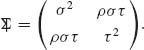
Make a linear transformation (X, Y) → (U, W) such that (U, W) are independent N(0, 1).
2.7.2 Let (X1, X2) have a bivariate normal distribution N(ξ, ![]() ). Define Y = α X1 + β X2.
). Define Y = α X1 + β X2.
2.7.3 The following is a normal regression model discussed, more generally, in Chapter 5. (x1, Y1), …, (xn, Yn) are n pairs in which x1, …, xn are preassigned constants and Y1, …, Yn independent random variables. According to the model, Yi ∼ N(α + β xi, σ2), i = 1, …, n. Let ![]() and
and
![]()
![]() and
and ![]() are called the least–squares estimates of α and β, respectively. Derive the joint distribution of
are called the least–squares estimates of α and β, respectively. Derive the joint distribution of ![]() . [We assume that Σ(xi –
. [We assume that Σ(xi – ![]() )2 > 0.]
)2 > 0.]
2.7.4 Suppose that X is an m–dimensional random vector and Y is an r–dimensional one, 1≤ r ≤ m. Furthermore, assume that the conditional distribution of X given Y is N(AY, ![]() ) where A is an m × r matrix of constants. In addition, let Y ∼ N(η, D).
) where A is an m × r matrix of constants. In addition, let Y ∼ N(η, D).
2.7.5 Let (Z1, Z2) have a standard bivariate normal distribution with coefficient of correlation ρ. Suppose that Z1 and Z2 are unobservable and that the observable random variables are
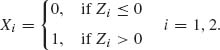
Let τ be the coefficient of correlation between X1 and X2. Prove that ρ = sin(π τ/2). [τ is called the tetrachoric (four–entry) correlation.]
2.7.6 Let (Z1, Z2) have a standard bivariate normal distribution with coefficient of correlation ρ = 1/2. Prove that P{Z1 ≥ 0, Z2 ≤ 0} = 1/6.
2.7.7 Let (Z1, Z2, Z3) have a standard trivariate normal distribution with a correlation matrix
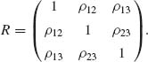
Consider the linear regression of Z1 on Z3, namely ![]() 1 = ρ13Z3 and the linear regression of Z2 on Z3, namely
1 = ρ13Z3 and the linear regression of Z2 on Z3, namely ![]() 2 = ρ23Z3. Show that the correlation between Z1 –
2 = ρ23Z3. Show that the correlation between Z1 – ![]() 1 and Z2 –
1 and Z2 – ![]() 2 is the partial correlation ρ12 · 3 given by (2.7.15).
2 is the partial correlation ρ12 · 3 given by (2.7.15).
2.7.8 Let (Z1, Z2) have a standard bivariate normal distribution with coefficient of correlation ρ. Let μrs = ![]() denote the mixed moment of order (r, s).
denote the mixed moment of order (r, s).
Show that
2.7.9 A commonly tabulated function for the standard bivariate normal distribution is the upper orthant probability
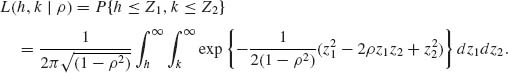
Show that
2.7.10 Suppose that X has a multinormal distribution N(ξ, ![]() ). Let X(n) = max{Xi}. Express the c.d.f. of X(n) in terms of the standard multinormal 1 ≤ i ≤ n
). Let X(n) = max{Xi}. Express the c.d.f. of X(n) in terms of the standard multinormal 1 ≤ i ≤ n
c.d.f., Φn(Z; R).
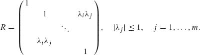
2.7.11 Let Z = (Z1, …, Zm)′ have a standard multinormal distribution whose correlation matrix R has elements
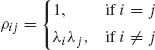
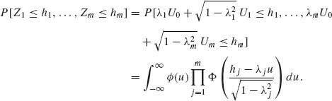
where |λi| ≤ 1 (i = 1, …, m). Prove that
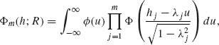
where ![]() (u) is the standard normal p.d.f. [Hint: Let U0, U1, …, Um be independent N(0, 1) and let
(u) is the standard normal p.d.f. [Hint: Let U0, U1, …, Um be independent N(0, 1) and let ![]() .]
.]
2.7.12 Let Z have a standard m–dimensional multinormal distribution with a correlation matrix R whose off–diagonal elements are ρ, 0 < ρ < 1. Show that
![]()
where 0 < a < ∞, a2 = 2ρ/(1–ρ). In particular, for ρ = 1/2, Φm0; R) = (1 + m)-1.
Section 2.8
2.8.1 Let X ∼ N(0, σ2) and Q = X2. Prove that Q ∼ σ2χ2[1] by deriving the m.g.f. of Q.
2.8.2 Consider the normal regression model (Problem 3, Section 2.7). The sum of squares of deviation around the fitted regression line is
![]()
where r is the sample coefficient of correlation, i.e.,
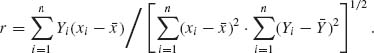
Prove that QY | X ∼ σ2χ2[n-2].
2.8.3 Let {Yij; i = 1, …, I, j = 1, …, J} be a set of random variables. Consider the following two models (of ANOVA, discussed in Section 4.6.2).
Model I: Yij are mutually independent, and for each i (i = 1, …, I)Yij ∼ N(ξi, σ2) for all j = 1, …, J. ξ1, …, ξI are constants.
Model II: For each i (i = 1, …, I) the conditional distribution of Yij given ξi is N(ξi, σ2) for all j = 1, …, J. Furthermore, given ξ1, …, ξI, Yij are conditionally independent. ξ1, …, ξI are independent random variables having the common distribution N(0, τ2). Define the quadratic forms
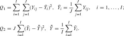
Determine the distributions of Q1 and Q2 under the two different models.
2.8.4 Prove that if X1 and X2 are independent and Xi ∼ χ2[νi;λi] i = 1, 2, then X1 + X2 ∼ χ2[ν1 + ν2;λ1+λ2].
Section 2.9
2.9.1 Consider the statistics Q1 and Q2 of Problem 3, Section 2.8. Check whether they are independent.
2.9.2 Consider Example 2.5. Prove that the least–squares estimator ![]() is independent of Q1.
is independent of Q1.
2.9.3 Let (X1, Y1), …, (Xn, Yn) be independent random vectors having a common bivariate normal distribution with V{X} = V{Y} =1. Let

and
![]()
where ρ, -1 < ρ < 1, is the correlation between X and Y. Prove that Q1 and Q2 are independent. [Hint: Consider the random variables Ui = Xi – ρ Yi, i = 1, …, n.]
2.9.4 Let X be an n × 1 random vector having a multinormal distribution N(μ 1, ![]() ) where
) where

J = 11′. Prove that ![]() and
and ![]() are independent and find their distribution. [Hint: Apply the Helmert orthogonal transformation Y = HX, where H is an n × n orthogonal matrix with first row vector equal to
are independent and find their distribution. [Hint: Apply the Helmert orthogonal transformation Y = HX, where H is an n × n orthogonal matrix with first row vector equal to ![]() .]
.]
Section 2.10
2.10.1 Let X1, …, Xn be independent random variables having a common exponential distribution E(λ), 0 < λ < ∞. Let X(1) ≤ … ≤ X(n) be the order statistics.
2.10.2 Let X1, …, Xn be independent random variables having an identical continuous distribution F(x). Let X(1) ≤ … ≤ X(n) be the order statistics. Find the distribution of U = (F(X(n)) – F(X(2)))/(F(X(n)) – F(X(1))).
2.10.3 Derive the p.d.f. of the range R = X(n) – X(1) of a sample of n = 3 independent random variables from a common N(μ, σ2) distribution.
2.10.4 Let X1, …, Xn, where n = 2m + 1, be independent random variables having a common rectangular distribution R(0, θ), 0 < θ < ∞. Define the statistics U = X(m) – X(1) and W = X(n) – X(m + 1). Find the joint p.d.f. of (U, W) and their coefficient of correlation.
2.10.5 Let X1, …, Xn be i.i.d. random variables having a common continuous distribution symmetric about x0 = μ. Let f(i)(x) denote the p.d.f. of the ith order statistic, i = 1, …, n. Show that f(r)(μ + x)= f(n – r + 1)(μ – x), all x, r = 1, …, n.
2.10.6 Let X(n) be the maximum of a sample of size n of independent identically distributed random variables having a standard exponential distribution E(1). Show that the c.d.f. of Yn = X(n) – log n converges, as n → ∞, to exp{–e–x}, which is the extreme–value distribution of Type I (Section 2.3.4). [This result can be generalized to other distributions too. Under some general conditions on the distribution of X, the c.d.f. of X(n) + log n converges to the extreme–value distribution of Type I (Galambos, 1978.)
2.10.7 Suppose that Xn, 1, …, Xn, k are k independent identically distributed random variables having the distribution of the maximum of a random sample of size n from R(0, 1). Let V =![]() . Show that the p.d.f. of V is (David, 1970, p. 22)
. Show that the p.d.f. of V is (David, 1970, p. 22)
![]()
Section 2.11
2.11.1 Let X ∼ t[10]. Determine the value of the coefficient of kurtosis γ = ![]() .
.
2.11.2 Consider the normal regression model (Problem 3, Section 2.7 and Problem 2, Section 2.8). The standard errors of the least–squares estimates are defined as
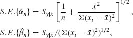
where ![]() = Qy | x/(n – 2). What are the distributions of
= Qy | x/(n – 2). What are the distributions of ![]() and of
and of ![]() ?
?
2.11.3 Let Φ(u) be the standard normal integral and let X ∼ (χ2[1])1/2. Prove that E{Φ(X)} = 3/4.
2.11.4 Derive the formulae (2.11.8)–(2.11.10).
2.11.5 Let X ∼ N(μ 1, ![]() ), with
), with ![]() , where
, where ![]() (see Problem 4, Section 2.9). Let
(see Problem 4, Section 2.9). Let ![]() and S be the (sample) mean and variance of the components of X.
and S be the (sample) mean and variance of the components of X.
2.11.6 Let t have the multivariate t–distribution t[ν ; ξ}, σ2R]. Show that the covariance matrix of t is ![]() .
.
Section 2.12
2.12.1 Derive the p.d.f. (2.12.2) of F[ν1, ν2].
2.12.2 Apply formulae (2.2.2) and (2.12.3) to derive the relationship between the binomial c.d.f. and that of the F–distribution, namely
(2.15.1) ![]()
Notice that this relationship can be used to compute the c.d.f. of a central–F distribution with both ν1 and ν2 even by means of the binomial distribution. For example, P{F[6, 8] ≤ 8/3} = B(3 | 6, ![]() ) = .89986.
) = .89986.
2.12.3 Derive formula (2.12.10).
2.12.4 Apply formula (2.12.15) to express the c.d.f. of F[2m, 2k; λ] as a Poisson mixture of binomial distributions.
Section 2.13
2.13.1 Find the expected value and the variance of the sample correlation r when the parameter is ρ.
2.13.2 Show that when ρ = 0 then the distribution of the sample correlation r is symmetric around zero.
2.13.3 Express the quantiles of the sample correlation r, when ρ = 0, in terms of those of t[n – 2].
Section 2.14
2.14.1 Show that the families of binomial, Poisson, negative–binomial, and gamma distributions are exponential type families. In each case, identify the canonical parameters and the natural parameter space.
2.14.2 Show that the family of bivariate normal distributions is a five–parameter exponential type. What are the canonical parameters and the canonical variables?
2.14.3 Let X ∼ N(μ, ![]() ) and Y ∼ N(μ,
) and Y ∼ N(μ, ![]() ) where X and Y are independent. Show that the joint distribution of (X, Y) is a curved exponential family.
) where X and Y are independent. Show that the joint distribution of (X, Y) is a curved exponential family.
2.14.4 Consider n independent random variables, where Xi ∼ P(μ (αi – αi-1)), (Poisson), (i = 1, …, n). Show that their joint p.d.f. belongs to a two–parameter exponential family. What are the canonical parameters and what are the canonical statistics? The parameter space Θ = {(μ, α): 0 < μ < ∞, 1 < α < ∞}.
2.14.5 Let T1, T2, …, Tn be i.i.d. random variables having an exponential distribution E(λ). Let 0 < t0 < ∞. We observed the censored variables X1, …, Xn where
![]()
i = 1, …, n. Show that the joint distribution of X1, …, Xn is a curved exponential family. What are the canonical statistics?
Section 2.15
2.15.1 Let X1, …, Xn be i.i.d. random variables having a binomial distribution B(1, θ). Compare the c.d.f. of ![]() n, for n = 10 and θ = .3 with the corresponding Edgeworth approximation.
n, for n = 10 and θ = .3 with the corresponding Edgeworth approximation.
2.15.2 Let X1, …, Xn be i.i.d. random variables having a Weibull distribution G1/α (λ, 1). Approximate the distribution of ![]() n by the Edgeworth approximation for n = 20, α = 2.5, λ = 1.
n by the Edgeworth approximation for n = 20, α = 2.5, λ = 1.
2.15.3 Approximate the c.d.f. of the Weibull, G1/α (λ, 1), when α = 2.5, λ = ![]() by an Edgeworth approximation with n = 1. Compare the exact c.d.f. to the approximation.
by an Edgeworth approximation with n = 1. Compare the exact c.d.f. to the approximation.
2.15.4 Let ![]() n be the sample mean of n i.i.d. random variables having a log–normal distribution, LN(μ, σ2). Determine the saddlepoint approximation to the p.d.f. of
n be the sample mean of n i.i.d. random variables having a log–normal distribution, LN(μ, σ2). Determine the saddlepoint approximation to the p.d.f. of ![]() n.
n.
PART IV: SOLUTIONS TO SELECTED PROBLEMS
2.2.2 Prove that 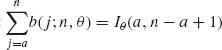 .
.

2.2.6 X ∼ Pascal(θ, ν), i.e.,
![]()
Let k = j – ν, k ≥ 0. Then
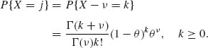
Let ψ = 1 – θ. Then
![]()
Thus, X – ν ∼ NB(ψ, ν) or X ∼ ν + NB(ψ, ν). The median of X is equal to ν + the median of NB(ψ, ν). Using the formula
![]()
median of NB(ψ, ν) = least n ≥ 0 such that Iθ (ν, n + 1) ≥ 0.5. Denote this median by n.5. Then X.5 = ν + n.5.
2.3.1 U ∼ R(0, 1). Y ∼ β-1(U | a, b). For 0 < y < 1
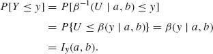
That is, β-1(U; a, b) ∼ β (a, b).
2.3.2 ![]() .
.
![]()
Hence, ![]() .
.
2.3.9 X ∼ LN(μ, σ2).
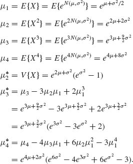
Coefficient of skewness β1 = ![]() .
.
![]()
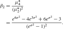
Coefficient of kurtosis
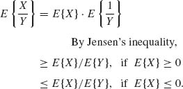
2.4.1 X, Y are independent r.v. P{Y > 0} = 1, E{|X|} < ∞.
2.4.4 X, Y are i.i.d. like N(0, 1). Find the distribution of R = X/Y.
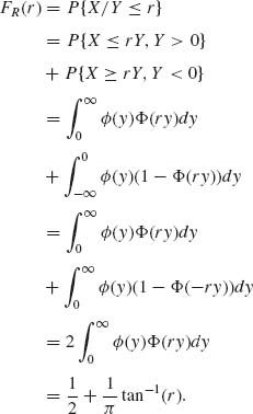
This is the standard Cauchy distribution with p.d.f.
![]()
Moments of R do not exist.
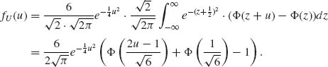
2.4.9 X, Y i.i.d. E(λ), U = X + Y, W = X – Y, U ∼ G(λ, 2), fU(u) = λ2 ue-λ u.
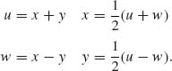
The Jacobian is
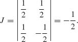
The joint p.d.f. of (U, W) is g(u, w) = ![]() , 0 < u < ∞, |w| < u. The conditional density of W given U is
, 0 < u < ∞, |w| < u. The conditional density of W given U is
![]()
That is, W | U ∼ R(–U, U).
![]()
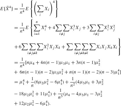
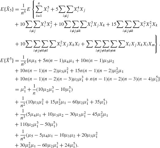
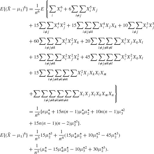
2.5.4 All moments exist. μi = E(Xi), i = 1, …, 4.
2.6.3 (X1, X2) has a bivariate NB(θ1, θ2, ν). The marginals X1 ∼ ![]() .
.
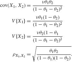
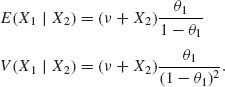
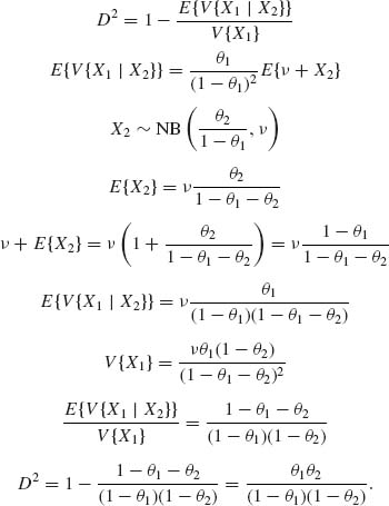
Notice that ![]() .
.
2.7.4
![]()
Hence, the m.g.f. of X is
![]()
Thus, X ∼ N(Aη, ![]() , + ADA′).
, + ADA′).
![]()
It follows that the conditional distribution of Y given X is
![]()
2.7.5
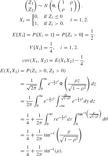
Hence,
![]()
The tetrachoric correlation is
![]()
or
![]()
2.7.11
Let U0, U1, …, Um be i.i.d. N(0, 1) random variables. Define Zj = λj U0 + ![]() = 1, …, m. Obviously, E{Zj} = 0, V{Zj} = 1, j = 1, …, m, and cov(Zi, Zj) = λiλj if i ≠ j. Finally, since U0, …, Um are independent
= 1, …, m. Obviously, E{Zj} = 0, V{Zj} = 1, j = 1, …, m, and cov(Zi, Zj) = λiλj if i ≠ j. Finally, since U0, …, Um are independent
2.10.1 X1, …, Xn are i.i.d. E(λ).
As shown in Example 2.12,

Thus,
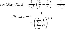
Also, as shown in Example 2.12, X(1) is independent of X(n)–X(1). Thus,
![]()
2.10.3 We have to derive the p.d.f. of R = X(3)–X(1), where X1, X2, X3 are i.i.d. N(μ, σ2). Write R = σ (Z(3)–Z(1)), where Z1, …, Z3 are i.i.d. N(0, 1). The joint density of (Z(1), Z(3)) is
![]()
where -∞ < z1 < z3 < ∞.
Let U = Z(3)–Z(1). The joint density of (Z(1), U) is

-∞ < z < ∞, 0 < u < ∞. Thus, the marginal density of U is
2.11.3
![]()
where U and X are independent. Hence,
![]()