CHAPTER 3
Sufficient Statistics and the Information in Samples
PART I: THEORY
3.1 INTRODUCTION
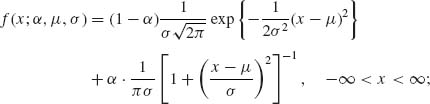
The problem of statistical inference is to draw conclusions from the observed sample on some characteristics of interest of the parent distribution of the random variables under consideration. For this purpose we formulate a model that presents our assumptions about the family of distributions to which the parent distribution belongs. For example, in an inventory management problem one of the important variables is the number of units of a certain item demanded every period by the customer. This is a random variable with an unknown distribution. We may be ready to assume that the distribution of the demand variable is Negative Binomial NB(![]() , ν). The statistical model specifies the possible range of the parameters, called the parameter space, and the corresponding family of distributions
, ν). The statistical model specifies the possible range of the parameters, called the parameter space, and the corresponding family of distributions ![]() . In this example of an inventory system, the model may be
. In this example of an inventory system, the model may be
![]()
Such a model represents the case where the two parameters, ![]() and ν, are unknown. The parameter space here is Θ = {(
and ν, are unknown. The parameter space here is Θ = {(![]() , ν); 0 <
, ν); 0 < ![]() < 1, 0 < ν < ∞ }. Given a sample of n independent and identically distributed (i.i.d.) random variables X1, …, Xn, representing the weekly demand, the question is what can be said on the specific values of
< 1, 0 < ν < ∞ }. Given a sample of n independent and identically distributed (i.i.d.) random variables X1, …, Xn, representing the weekly demand, the question is what can be said on the specific values of ![]() and ν from the observed sample?
and ν from the observed sample?
Every sample contains a certain amount of information on the parent distribution. Intuitively we understand that the larger the number of observations in the sample (on i.i.d. random variables) the more information it contains on the distribution under consideration. Later in this chapter we will discuss two specific information functions, which are used in statistical design of experiments and data analysis. We start with the investigation of the question whether the sample data can be condensed by computing first the values of certain statistics without losing information. If such statistics exist they are called sufficient statistics. The term statistic will be used to indicate a function of the (observable) random variables that does not involve any function of the unknown parameters. The sample mean, sample variance, the sample order statistics, etc., are examples of statistics. As will be shown, the notion of sufficiency of statistics is strongly dependent on the model under consideration. For example, in the previously mentioned inventory example, as will be established later, if the value of the parameter ν is known, a sufficient statistic is the sample mean ![]() . On the other hand, if ν is unknown, the sufficient statistic is the order statistic (X(1), …, X(n)). When ν is unknown, the sample mean
. On the other hand, if ν is unknown, the sufficient statistic is the order statistic (X(1), …, X(n)). When ν is unknown, the sample mean ![]() by itself does not contain all the information on
by itself does not contain all the information on ![]() and ν. In the following section we provide a definition of sufficiency relative to a specified model and give a few examples.
and ν. In the following section we provide a definition of sufficiency relative to a specified model and give a few examples.
3.2 DEFINITION AND CHARACTERIZATION OF SUFFICIENT STATISTICS
3.2.1 Introductory Discussion
Let X = (X1, …, Xn) be a random vector having a joint c.d.f. Fθ (x) belonging to a family ![]() = {Fθ (x); θ
= {Fθ (x); θ ![]() Θ }. Such a random vector may consist of n i.i.d. variables or of dependent random variables. Let T(X) = (T1(X), …, Tr(X))′, 1 ≤ r ≤ n be a statistic based on X. T could be real (r = 1) or vector valued (r > 1). The transformations Tj(X), j = 1, …, r are not necessarily one–to–one. Let f(x; θ) denote the (joint) probability density function (p.d.f.) of X. In our notation here Ti(X) is a concise expression for Ti(X1, …, Xn). Similarly, Fθ (x) and f(x; θ) represent the multivariate functions Fθ (x1, …, xn) and f(x1, …, xn;θ). As in the previous chapter, we assume throughout the present chapter that all the distribution functions belonging to the same family are either absolutely continuous, discrete, or mixtures of the two types.
Θ }. Such a random vector may consist of n i.i.d. variables or of dependent random variables. Let T(X) = (T1(X), …, Tr(X))′, 1 ≤ r ≤ n be a statistic based on X. T could be real (r = 1) or vector valued (r > 1). The transformations Tj(X), j = 1, …, r are not necessarily one–to–one. Let f(x; θ) denote the (joint) probability density function (p.d.f.) of X. In our notation here Ti(X) is a concise expression for Ti(X1, …, Xn). Similarly, Fθ (x) and f(x; θ) represent the multivariate functions Fθ (x1, …, xn) and f(x1, …, xn;θ). As in the previous chapter, we assume throughout the present chapter that all the distribution functions belonging to the same family are either absolutely continuous, discrete, or mixtures of the two types.
Definition of Sufficiency. Let ![]() be a family of distribution functions and let X = (X1, …, Xn) be a random vector having a distribution in
be a family of distribution functions and let X = (X1, …, Xn) be a random vector having a distribution in ![]() . A statistic T(X) is called sufficient with respect to
. A statistic T(X) is called sufficient with respect to ![]() if the conditional distribution of X given T(X) is the same for all the elements of
if the conditional distribution of X given T(X) is the same for all the elements of ![]() .
.
Accordingly, if the joint p.d.f. of X, f(x; θ), depends on a parameter θ and T(X) is a sufficient statistic with respect to ![]() , the conditional p.d.f. h(x| t) of X given {T(X) = t} is independent of θ. Since f(x;θ) = h(x| t)g(t; θ), where g(t; θ) is the p.d.f. of T(x), all the information on θ in x is summarized in T(x).
, the conditional p.d.f. h(x| t) of X given {T(X) = t} is independent of θ. Since f(x;θ) = h(x| t)g(t; θ), where g(t; θ) is the p.d.f. of T(x), all the information on θ in x is summarized in T(x).
The process of checking whether a given statistic is sufficient for some family following the above definition may be often very tedious. Generally the identification of sufficient statistics is done by the application of the following theorem. This celebrated theorem was given first by Fisher (1922) and Neyman (1935). We state the theorem here in terms appropriate for families of absolutely continuous or discrete distributions. For more general formulations see Section 3.2.2. For the purposes of our presentation we require that the family of distributions ![]() consists of
consists of
 for all θ
 The families of discrete or absolutely continuous distributions discussed in Chapter 2 are all regular.
Theorem 3.2.1 (The Neyman–Fisher Factorization Theorem). Let X be a random vector having a distribution belonging to a regular family ![]() and having a joint p.d.f. f(x; θ), θ
and having a joint p.d.f. f(x; θ), θ ![]() Θ. A statistic T(X) is sufficient for
Θ. A statistic T(X) is sufficient for ![]() if and only if
if and only if
where K(x) ≥ 0 is independent of θ and g(T(x); θ) ≥ 0 depends on x only through T(x).
Proof. We provide here a proof for the case of discrete distributions.
We show that (3.2.1) implies that the conditional distribution of X given {T(X) = t} is independent of θ. The (marginal) p.d.f. of T(X) is, according to (3.2.1),
(3.2.2) 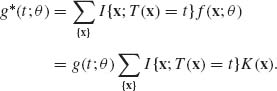
The joint p.d.f. of X and T(X) is
(3.2.3) ![]()
Hence, the conditional p.d.f. of X, given {T(X) = t at every point t such that g* (t; θ) > 0, is
(3.2.4) 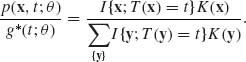
This proves that T(X) is sufficient for ![]() .
.
Suppose that T(X) is sufficient for ![]() . Then, for every t at which the (marginal) p.d.f. of T(X), g* (t;θ), is positive we have,
. Then, for every t at which the (marginal) p.d.f. of T(X), g* (t;θ), is positive we have,
where B(x) ≥ 0 is independent of θ. Moreover, ![]() since (3.2.5) is a conditional p.d.f. Thus, for every x,
since (3.2.5) is a conditional p.d.f. Thus, for every x,
(3.2.6) ![]()
Finally, since for every x,
(3.2.7) ![]()
we obtain that
(3.2.8) ![]() QED
QED
3.2.2 Theoretical Formulation
3.2.2.1 Distributions and Measures
We generalize the definitions and proofs of this section by providing measure–theoretic formulation. Some of these concepts were discussed in Chapter 1. This material can be skipped by students who have not had real analysis.
Let (Ω, ![]() , P) be a probability space. A random variable X is a finite real value measurable function on this probability space, i.e., X: Ω →
, P) be a probability space. A random variable X is a finite real value measurable function on this probability space, i.e., X: Ω → ![]() . Let
. Let ![]() be the sample space (range of X), i.e.,
be the sample space (range of X), i.e., ![]() = X(Ω). Let
= X(Ω). Let ![]() be the Borel σ–field on
be the Borel σ–field on ![]() , and consider the probability space (
, and consider the probability space (![]() ,
, ![]() , PX) where, for each B
, PX) where, for each B ![]()
![]() , PX{B} = P{X−1(B)}. Since X is a random variable,
, PX{B} = P{X−1(B)}. Since X is a random variable, ![]() X = {A: A = X−1(B), B
X = {A: A = X−1(B), B ![]()
![]() }
} ![]()
![]() .
.
The distribution function of X is
(3.2.9) ![]()
Let X1, X2, …, Xn be n random variables defined on the same probability space (Ω, ![]() , P). The joint distribution of X = (X1, …, Xn)′ is a real value function of
, P). The joint distribution of X = (X1, …, Xn)′ is a real value function of ![]() n defined as
n defined as
(3.2.10) 
Consider the probability space (![]() (n),
(n), ![]() (n), P(n)) where
(n), P(n)) where ![]() (n) =
(n) = ![]() × ··· ×
× ··· × ![]() ,
, ![]() (n) =
(n) = ![]() × ··· ×
× ··· × ![]() (or the Borel σ–field generated by the intervals (−∞, x1] × ··· (−∞, xn], (x1, …, xn)
(or the Borel σ–field generated by the intervals (−∞, x1] × ··· (−∞, xn], (x1, …, xn) ![]()
![]() n) and for B
n) and for B ![]()
![]() (n)
(n)
(3.2.11) ![]()
A function h: ![]() (n) →
(n) → ![]() is said to be
is said to be ![]() (n)–measurable if the sets h−1((−∞, ζ]) are in
(n)–measurable if the sets h−1((−∞, ζ]) are in ![]() (n) for all −∞ < ζ < ∞. By the notation h
(n) for all −∞ < ζ < ∞. By the notation h![]()
![]() (n) we mean that h is
(n) we mean that h is ![]() (n)–measurable.
(n)–measurable.
A random sample of size n is the realization of n i.i.d. random variables (see Chapter 2 for definition of independence).
To economize in notation, we will denote by bold x the vector (x1, …, xn), and by F(x) the joint distribution of (X1, …, Xn). Thus, for all B ![]()
![]() (n),
(n),
(3.2.12) ![]()
This is a probability measure on (![]() (n), B(n)) induced by F(x). Generally, a σ–finite measure μ on
(n), B(n)) induced by F(x). Generally, a σ–finite measure μ on ![]() (n) is a nonnegative real value set function, i.e., μ:
(n) is a nonnegative real value set function, i.e., μ: ![]() (n) → [0, ∞], such that
(n) → [0, ∞], such that
The Lebesque measure ![]() is a σ–finite measure on B(n).
is a σ–finite measure on B(n).
If there is a countable set of marked points in ![]() n, S = {x1, x2, x3, … }, the counting measure is
n, S = {x1, x2, x3, … }, the counting measure is
![]()
N(B; S) is a σ–finite measure, and for any finite real value function g(x)
![]()
Notice that if B is such that N(B; S) = 0 then ![]() B g(x)d N(x; S) = 0. Similarly, if B is such that
B g(x)d N(x; S) = 0. Similarly, if B is such that ![]() B dx = 0 then, for any positive integrable function g(x),
B dx = 0 then, for any positive integrable function g(x), ![]() B g(x)dx = 0. Moreover, ν (B) =
B g(x)dx = 0. Moreover, ν (B) = ![]() B g(x)d x and λ (B) =
B g(x)d x and λ (B) = ![]() B g(x)d N(x; S) are σ–finite measures on (
B g(x)d N(x; S) are σ–finite measures on (![]() (n),
(n), ![]() (n)).
(n)).
Let ν and μ be two σ–finite measures defined on (![]() (n),
(n), ![]() (n)). We say that ν is absolutely continuous with respect to μ if μ (B) = 0 implies that ν (B) = 0. We denote this relationship by ν
(n)). We say that ν is absolutely continuous with respect to μ if μ (B) = 0 implies that ν (B) = 0. We denote this relationship by ν ![]() μ. If ν
μ. If ν ![]() μ and μ
μ and μ ![]() ν, we say that ν and μ are equivalent, ν ≡ μ. We will use the notation F
ν, we say that ν and μ are equivalent, ν ≡ μ. We will use the notation F ![]() μ if the probability measure PF is absolutely continuous with respect to μ. If F
μ if the probability measure PF is absolutely continuous with respect to μ. If F ![]() μ there exists a nonnegative function f(x), which is
μ there exists a nonnegative function f(x), which is ![]() measurable, satisfying
measurable, satisfying
(3.2.13) ![]()
f(x) is called the (Radon–Nikodym) derivative of F with respect to μ or the generalized density p.d.f. of F(x). We write
(3.2.14) ![]()
or
(3.2.15) ![]()
As discussed earlier, a statistical model is represented by a family ![]() of distribution functions Fθ on
of distribution functions Fθ on ![]() (n), θ
(n), θ ![]() Θ. The family
Θ. The family ![]() is dominated by a σ–finite measure μ if Fθ
is dominated by a σ–finite measure μ if Fθ ![]() μ, for each θ
μ, for each θ ![]() Θ.
Θ.
We consider only models of dominated families. A theorem in measure theory states that if ![]()
![]() μ then there exists a countable sequence
μ then there exists a countable sequence ![]()
![]()
![]() such that
such that
(3.2.16) ![]()
induces a probability measure P*, which dominates ![]() .
.
A statistic T(X) is a measurable function of the data X. More precisely, let T: ![]() (n) →
(n) → ![]() (k), k ≥ 1 and let
(k), k ≥ 1 and let ![]() (k) be the Borel σ–field of subsets of
(k) be the Borel σ–field of subsets of ![]() (k). The function T(X) is a statistic if, for every C
(k). The function T(X) is a statistic if, for every C ![]()
![]() (k), T−1(C)
(k), T−1(C) ![]()
![]() (n). Let
(n). Let ![]() T = {B: B = T−1(C) for C
T = {B: B = T−1(C) for C ![]()
![]() (k)}. The probability measure PT on
(k)}. The probability measure PT on ![]() (k), induced by PX, is given by
(k), induced by PX, is given by
(3.2.17) ![]()
Thus, the induced distribution function of T is FT(t), where t ![]()
![]() k and
k and
(3.2.18) ![]()
If F ![]() μ then FT
μ then FT ![]() μT, where μT(C) = μ (T−1(C)) for all C
μT, where μT(C) = μ (T−1(C)) for all C ![]()
![]() (k). The generalized density (p.d.f.) of T with respect to μT is gT(t) where
(k). The generalized density (p.d.f.) of T with respect to μT is gT(t) where
(3.2.19) ![]()
If h(x) is ![]() (n) measurable and
(n) measurable and ![]() |h(x)| dF(x) < ∞, then the conditional expectation of h(X) given {T(X) = t} is a
|h(x)| dF(x) < ∞, then the conditional expectation of h(X) given {T(X) = t} is a ![]() T measurable function, EF{h(X)| T(X) = t}, for which
T measurable function, EF{h(X)| T(X) = t}, for which
(3.2.20) 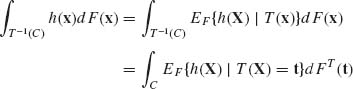
for all C ![]()
![]() (k). In particular, if C =
(k). In particular, if C = ![]() (k) we obtain the law of the iterated expectation; namely
(k) we obtain the law of the iterated expectation; namely
(3.2.21) ![]()
Notice that EF{h(X) | T(X)} assumes a constant value on the coset A(t) = {x: T(x) = t} = T−1({t}), t ![]()
![]() (k).
(k).
3.2.2.2 Sufficient Statistics
Consider a statistical model (![]() (n),
(n), ![]() (n),
(n), ![]() ) where
) where ![]() is a family of joint distributions of the random sample. A statistic T: (
is a family of joint distributions of the random sample. A statistic T: (![]() (n),
(n), ![]() (n),
(n), ![]() ) → (
) → (![]() (k),
(k), ![]() (k),
(k), ![]() T) is called sufficient for
T) is called sufficient for ![]() if, for all B
if, for all B ![]()
![]() (n), PF{B| T(X) = t} = p(B; t) for all F
(n), PF{B| T(X) = t} = p(B; t) for all F ![]()
![]() . That is, the conditional distribution of X given T(X) is the same for all F in
. That is, the conditional distribution of X given T(X) is the same for all F in ![]() . Moreover, for a fixed t, p(B; t) is
. Moreover, for a fixed t, p(B; t) is ![]() (n) measurable and for a fixed B, p(B; t) is
(n) measurable and for a fixed B, p(B; t) is ![]() (k) measurable.
(k) measurable.
Theorem 3.2.2 Let (![]() (n),
(n), ![]() (n),
(n), ![]() ) be a statistical model and
) be a statistical model and ![]()
![]() μ. Let
μ. Let ![]()
![]()
![]() such that F*(x) =
such that F*(x) =  and
and ![]()
![]() P*. Then T(X) is sufficient for
P*. Then T(X) is sufficient for ![]() if and only if for each θ
if and only if for each θ ![]() Θ there exists a
Θ there exists a ![]() T measurable function gθ (T(x)) such that, for each B
T measurable function gθ (T(x)) such that, for each B ![]()
![]() (n)
(n)
(3.2.22) ![]()
i.e.,
(3.2.23) ![]()
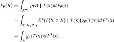
Proof. (i) Assume that T(X) is sufficient for ![]() . Accordingly, for each B
. Accordingly, for each B ![]()
![]() (n),
(n),
![]()
for all θ ![]() Θ. Fix B in
Θ. Fix B in ![]() (n) and let C
(n) and let C ![]()
![]() (k).
(k).
![]()
for each θ ![]() Θ. In particular,
Θ. In particular,
![]()
By the Radon–Nikodym Theorem, since Fθ ![]() F* for each θ, there exists a
F* for each θ, there exists a ![]() T measurable function gθ (T(X)) so that, for every C
T measurable function gθ (T(X)) so that, for every C ![]()
![]() (k),
(k),
![]()
Now, for B ![]()
![]() (n) and θ
(n) and θ ![]() Θ,
Θ,
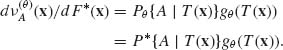
Hence, dFθ (x)/d F* (x) = gθ (T(x)), which is ![]() T measurable.
T measurable.
(ii) Assume that there exists a ![]() T measurable function gθ (T(x)) so that, for each θ
T measurable function gθ (T(x)) so that, for each θ ![]() Θ,
Θ,
![]()
Let A ![]()
![]() (n) and define the σ–finite measure
(n) and define the σ–finite measure ![]() . Thus,
. Thus,
Thus, Pθ {A| T(X)} = P*{A| T(X)} for all θ ![]() Θ. Therefore T is a sufficient statistic. QED
Θ. Therefore T is a sufficient statistic. QED
Theorem 3.2.3 (Abstract Formulation of the Neyman–Fisher Factorization Theorem) Let (![]() (n),
(n), ![]() (n),
(n), ![]() ) be a statistical model with
) be a statistical model with ![]()
![]() μ. Then T(X) is sufficient for
μ. Then T(X) is sufficient for ![]() if and only if
if and only if
(3.2.24) ![]()
where h ≥ 0 and h ![]()
![]() (n), gθ
(n), gθ ![]()
![]() T.
T.
Proof. Since ![]()
![]() μ,
μ, ![]()
![]()
![]() , such that F*(x) =
, such that F*(x) = ![]() dominates
dominates ![]() . Hence, by the previous theorem, T(X) is sufficient for
. Hence, by the previous theorem, T(X) is sufficient for ![]() if and only if there exists a
if and only if there exists a ![]() T measurable function gθ (T(x)) so that
T measurable function gθ (T(x)) so that
![]()
Let fθn(x) = d Fθn(x)/dμ (x) and set h(x) = ![]() . The function h(x)
. The function h(x) ![]()
![]() (n) and
(n) and
![]() QED
QED
3.3 LIKELIHOOD FUNCTIONS AND MINIMAL SUFFICIENT STATISTICS
Consider a vector X = (X1, …, Xn)′ of random variables having a joint c.d.f. Fθ (x) belonging to a family ![]() = {Fθ (x); θ
= {Fθ (x); θ ![]() Θ }. It is assumed that
Θ }. It is assumed that ![]() is a regular family of distributions, i.e.,
is a regular family of distributions, i.e., ![]()
![]() μ, and, for each θ
μ, and, for each θ ![]() Θ, there exists f(x;θ) such that
Θ, there exists f(x;θ) such that
![]()
f(x;θ) is the joint p.d.f. of X with respect to μ (x). We define over the parameter space Θ a class of functions L(θ; X) called likelihood functions. The likelihood function of θ associated with a vector of random variables X is defined up to a positive factor of proportionality as
The factor of proportionality in (3.3.1) may depend on X but not on θ. Accordingly, we say that two likelihood functions L1(θ ;X) and L2(θ ; X) are equivalent, i.e., L1(θ ; X) ∼ L2(θ ;X), if L1(θ ;X) = A(X) L2(θ ; X) where A(X) is a positive function independent of θ. For example, suppose that X = (X1, …, Xn)′ is a vector of i.i.d. random variables having a N(θ, 1) distribution, −-∞ < θ < ∞. The likelihood function of θ can be defined as
(3.3.2) 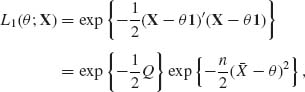
where ![]() and
and ![]() and 1′ = (1, …, 1) or as
and 1′ = (1, …, 1) or as
(3.3.3) ![]()
where ![]() . We see that for a given value of X, L1(θ ; X) ∼ L2(θ ; X). All the equivalent versions of a likelihood function L(θ; X) belong to the same equivalence class. They all represent similar functions of θ.
. We see that for a given value of X, L1(θ ; X) ∼ L2(θ ; X). All the equivalent versions of a likelihood function L(θ; X) belong to the same equivalence class. They all represent similar functions of θ.
If S(X) is a statistic having a p.d.f. gS(s; θ), (θ ![]() Θ), then the likelihood function of θ given S(X) = s is LS(θ; s)
Θ), then the likelihood function of θ given S(X) = s is LS(θ; s) ![]() gS(s; θ). LS(θ; s) may or may not have a shape similar to L(θ; X). From the Factorization Theorem we obtain that if L(θ; X)∼ LS(θ; S(X)), for all X, then S(X) is a sufficient statistic for
gS(s; θ). LS(θ; s) may or may not have a shape similar to L(θ; X). From the Factorization Theorem we obtain that if L(θ; X)∼ LS(θ; S(X)), for all X, then S(X) is a sufficient statistic for ![]() . The information on θ given by X can be reduced to S(X) without changing the factor of the likelihood function that depends on θ. This factor is called the kernel of the likelihood function. In terms of the above example, if T(X) =
. The information on θ given by X can be reduced to S(X) without changing the factor of the likelihood function that depends on θ. This factor is called the kernel of the likelihood function. In terms of the above example, if T(X) = ![]() , since
, since ![]() ∼ N
∼ N ![]() , LT(X)(θ; t) = exp
, LT(X)(θ; t) = exp ![]() . Thus, for all x such that T(x) = t, LX(θ; t) ∼ L1(θ; x) ∼ L2(θ; x).
. Thus, for all x such that T(x) = t, LX(θ; t) ∼ L1(θ; x) ∼ L2(θ; x). ![]() is indeed a sufficient statistic. The likelihood function LT(θ ; T(x)) associated with any sufficient statistic for
is indeed a sufficient statistic. The likelihood function LT(θ ; T(x)) associated with any sufficient statistic for ![]() is equivalent to the likelihood function L(θ; x) associated with X. Thus, if T(X) is a sufficient statistic, then the likelihood ratio
is equivalent to the likelihood function L(θ; x) associated with X. Thus, if T(X) is a sufficient statistic, then the likelihood ratio
![]()
is independent of θ. A sufficient statistic T(X) is called minimal if it is a function of any other sufficient statistic S(X). The question is how to determine whether a sufficient statistic T(X) is minimal sufficient.
Every statistic S(X) induces a partition of the sample space χ(n) of the observable random vector X. Such a partition is a collection of disjoint sets whose union is χ(n). Each set in this partition is determined so that all its elements yield the same value of S(X). Conversely, every partition of χ(n) corresponds to some function of X. Consider now the partition whose sets contain only x points having equivalent likelihood functions. More specifically, let x0 be a point in χ(n). A coset of x0 in this partition is
(3.3.4) ![]()
The partition of χ(n) is obtained by varying x0 over all the points of χ(n). We call this partition the equivalent–likelihood partition. For example, in the N(θ, 1) case −∞ < θ < ∞, each coset consists of vectors x having the same mean ![]() =
= ![]() 1′x. These means index the cosets of the equivalent–likelihood partitions. The statistic T(X) corresponding to the equivalent–likelihood partition is called the likelihood statistic. This statistic is an index of the likelihood function L(θ; x). We show now that the likelihood statistic T(X) is a minimal sufficient statistic (m.s.s.).
1′x. These means index the cosets of the equivalent–likelihood partitions. The statistic T(X) corresponding to the equivalent–likelihood partition is called the likelihood statistic. This statistic is an index of the likelihood function L(θ; x). We show now that the likelihood statistic T(X) is a minimal sufficient statistic (m.s.s.).
Let x(1) and x(2) be two different points and let T(x) be the likelihood statistic. Then, T(x(1)) = T(x(2)) if and only if L(θ; x(1)) ∼ L(θ ;x(2)). Accordingly, L(θ; X) is a function of T(X), i.e., f(X;θ) = A(X) g*(T(X); θ). Hence, by the Factorization Theorem, T(X) is a sufficient statistic. If S(X) is any other sufficient statistic, then each coset of S(X) is contained in a coset of T(X). Indeed, if x(1) and x(2) are such that S(x(1)) = S(x(2)) and f(x(i), θ) > 0 (i = 1,2), we obtain from the Factorization Theorem that f(x(1); θ) = k(x(1)) g(S(x(1)); θ) = k(x(1))g(S(x(2)); θ) = k(x(1)) f(x(2); θ)/k(x(2)), where k(x(2)) > 0. That is, L(θ; X(1)) ∼ L(θ; X(2)) and hence T(X(1)) = T(X(2)). This proves that T(X) is a function of S(X) and therefore minimal sufficient.
The minimal sufficient statistic can be determined by determining the likelihood statistic or, equivalently, by determining the partition of χ(n) having the property that f(x(1); θ)/f(x(2); θ) is independent of θ for every two points at the same coset.
3.4 SUFFICIENT STATISTICS AND EXPONENTIAL TYPE FAMILIES
In Section 2.16 we discussed the k–parameter exponential type family of distributions. If X1, …, Xn are i.i.d. random variables having a k–parameter exponential type distribution, then the joint p.d.f. of X = (X1, …, Xn), in its canonical form, is
(3.4.1) 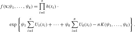
It follows that  is a sufficient statistic. The statistic T(X) is minimal sufficient if the parameters {
![]() 1, …,
1, …, ![]() k} are linearly independent. Otherwise, by reparametrization we can reduce the number of natural parameters and obtain an m.s.s. that is a function of T(X).
k} are linearly independent. Otherwise, by reparametrization we can reduce the number of natural parameters and obtain an m.s.s. that is a function of T(X).
Dynkin (1951) investigated the conditions under which the existence of an m.s.s., which is a nontrivial reduction of the sample data, implies that the family of distributions, ![]() , is of the exponential type. The following regularity conditions are called Dynkin’s Regularity Conditions. In Dynkin’s original paper, condition (iii) required only piecewise continuous differentiability. Brown (1964) showed that it is insufficient. We phrase (iii) as required by Brown.
, is of the exponential type. The following regularity conditions are called Dynkin’s Regularity Conditions. In Dynkin’s original paper, condition (iii) required only piecewise continuous differentiability. Brown (1964) showed that it is insufficient. We phrase (iii) as required by Brown.
Dynkin’s Regularity Conditions
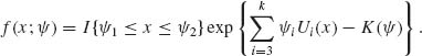
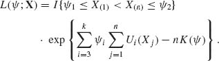
Theorem 3.4.1 (Dynkin’s). If the family ![]() is regular in the sense of Dynkin, and if for a sample of n ≥ k i.i.d. random variables U1(X), …, Uk(X) are linearly independent sufficient statistics, then the p.d.f. of X is
is regular in the sense of Dynkin, and if for a sample of n ≥ k i.i.d. random variables U1(X), …, Uk(X) are linearly independent sufficient statistics, then the p.d.f. of X is
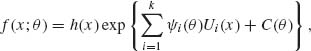
where the functions ![]() 1 (θ), …,
1 (θ), …, ![]() k(θ) are linearly independent.
k(θ) are linearly independent.
For a proof of this theorem and further reading on the subject, see Dynkin (1951), Brown (1964), Denny (1967, 1969), Tan (1969), Schmetterer (1974, p. 215), and Zacks (1971, p. 60). The connection between sufficient statistics and the exponential family was further investigated by Borges and Pfanzagl (1965), and Pfanzagl (1972). A one dimensional version of the theorem is proven in Schervish (1995, p. 109).
3.5 SUFFICIENCY AND COMPLETENESS
A family of distribution functions ![]() = {Fθ (x);θ
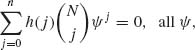
= {Fθ (x);θ ![]() Θ } is called complete if, for any integrable function h(X),
Θ } is called complete if, for any integrable function h(X),
(3.5.1) ![]()
implies that Pθ [h(X) = 0] = 1 for all θ ![]() Θ.
Θ.
A statistic T(X) is called complete sufficient statistic if it is sufficient for a family ![]() , and if the family
, and if the family ![]() T of all the distributions of T(X) corresponding to the distributions in
T of all the distributions of T(X) corresponding to the distributions in ![]() is complete.
is complete.
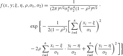
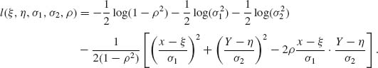
Minimal sufficient statistics are not necessarily complete. To show it, consider the family of distributions of Example 3.6 with ξ1 = ξ2 = ξ. It is a four–parameter, exponential–type distribution and the m.s.s. is
The family ![]() T is incomplete since
T is incomplete since 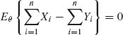 for all θ = (ξ, σ1, σ2). But , all θ. The reason for this incompleteness is that when ξ1 = ξ2 the four natural parameters are not independent. Notice that in this case the parameter space Ω = {
 ![]() = (
= (![]() 1,
1, ![]() 2,
2, ![]() 3,
3, ![]() 4);
4); ![]() 1 =
1 = ![]() 2
2 ![]() 3/
3/![]() 4} is three–dimensional.
4} is three–dimensional.
Theorem 3.5.1 If the parameter space Ω corresponding to a k–parameter exponential type family is k–dimensional, then the family of the minimal sufficient statistic is complete.
The proof of this theorem is based on the analyticity of integrals of the type (2.16.4). For details, see Schervish (1995, p. 108).
From this theorem we immediately deduce that the following families are complete.
We define now a weaker notion of boundedly complete families. These are families for which if h(x) is a bounded function and Eθ {h(X)} = 0, for all θ ![]() Θ, then Pθ {h(x) = 0} = 1, for all θ
Θ, then Pθ {h(x) = 0} = 1, for all θ ![]() Θ. For an example of a boundedly complete family that is incomplete, see Fraser (1957, p. 25).
Θ. For an example of a boundedly complete family that is incomplete, see Fraser (1957, p. 25).
Theorem 3.5.2 (Bahadur). If T(X) is a boundedly complete sufficient statistic, then T(X) is minimal.
Proof. Suppose that S(X) is a sufficient statistic. If S(X) = ![]() (T(X)) then, for any Borel set B
(T(X)) then, for any Borel set B ![]()
![]() ,
,
![]()
Define
![]()
By the law of iterated expectation, Eθ {h(T)} = 0, for all θ ![]() Θ. But since T(X) is boundedly complete,
Θ. But since T(X) is boundedly complete,
![]()
Hence, T ![]()
![]() S, which means that T is a function of S. Hence T(X) is an m.s.s. QED
S, which means that T is a function of S. Hence T(X) is an m.s.s. QED
3.6 SUFFICIENCY AND ANCILLARITY
A statistic A(X) is called ancillary if its distribution does not depend on the particular parameter(s) specifying the distribution of X. For example, suppose that X∼ N(θ 1n, In), −∞ < θ < ∞. The statistic U = (X2 − X1, …, Xn−X1) is distributed like N(On−1, In−1 + Jn−1). Since the distribution of U does not depend on θ, U is ancillary for the family ![]() = {N(θ 1, I), −∞ < θ < ∞ }. If S(X) is a sufficient statistic for a family
= {N(θ 1, I), −∞ < θ < ∞ }. If S(X) is a sufficient statistic for a family ![]() , the inference on θ can be based on the likelihood based on S. If fS(s; θ) is the p.d.f. of S, and if A(X) is ancillary for
, the inference on θ can be based on the likelihood based on S. If fS(s; θ) is the p.d.f. of S, and if A(X) is ancillary for ![]() , with p.d.f. h(a), one could write
, with p.d.f. h(a), one could write
(3.6.1) ![]()
where ![]() (s | a) is the conditional p.d.f. of S given {A = a}. One could claim that, for inferential objectives, one should consider the family of conditional p.d.f.s
(s | a) is the conditional p.d.f. of S given {A = a}. One could claim that, for inferential objectives, one should consider the family of conditional p.d.f.s ![]() S|A ={
S|A ={![]() (s | a), θ
(s | a), θ ![]() Θ }. However, the following theorem shows that if S is a complete sufficient statistic, conditioning on A(X) does not yield anything different, since pS(s; θ) =
Θ }. However, the following theorem shows that if S is a complete sufficient statistic, conditioning on A(X) does not yield anything different, since pS(s; θ) = ![]() (s | a), with probability one for each θ
(s | a), with probability one for each θ ![]() Θ.
Θ.
Theorem 3.6.1 (Basu’s Theorem). Let X = (X1, …, Xn)′ be a vector of i.i.d. random variables with a common distribution belonging to ![]() = {Fθ (x), θ
= {Fθ (x), θ ![]() Θ }. Let T(X) be a boundedly complete sufficient statistic for
Θ }. Let T(X) be a boundedly complete sufficient statistic for ![]() . Furthermore, suppose that A(X) is an ancillary statistic. Then T(X) and A(X) are independent.
. Furthermore, suppose that A(X) is an ancillary statistic. Then T(X) and A(X) are independent.
Proof. Let C ![]()
![]() A, where
A, where ![]() A is the Borel σ–subfield induced by A(X). Since the distribution of A(X) is independent of θ, we can determine P{A(X)
A is the Borel σ–subfield induced by A(X). Since the distribution of A(X) is independent of θ, we can determine P{A(X) ![]() C} without any information on θ. Moreover, the conditional probability P{A(X)
C} without any information on θ. Moreover, the conditional probability P{A(X) ![]() C | T(X)} is independent of θ since T(X) is a sufficient statistic. Hence, P{A(X)
C | T(X)} is independent of θ since T(X) is a sufficient statistic. Hence, P{A(X) ![]() C | T(X)} − P{A(X)
C | T(X)} − P{A(X) ![]() C} is a statistic depending on T(X). According to the law of the iterated expectation,
C} is a statistic depending on T(X). According to the law of the iterated expectation,
(3.6.2) ![]()
Finally, since T(x) is boundedly complete,
(3.6.3) ![]()
with probability one for each θ. Thus, A(X) and T(X) are independent. QED
From Basu’s Theorem, we can deduce that only if the sufficient statistic S(X) is incomplete for ![]() , then an inference on θ, conditional on an ancillary statistic, can be meaningful. An example of such inference is given in Example 3.10.
, then an inference on θ, conditional on an ancillary statistic, can be meaningful. An example of such inference is given in Example 3.10.
3.7 INFORMATION FUNCTIONS AND SUFFICIENCY
In this section, we discuss two types of information functions used in statistical analysis: the Fisher information function and the Kullback–Leibler information function. These two information functions are somewhat related but designed to fulfill different roles. The Fisher information function is applied in various estimation problems, while the Kullback–Leibler information function has direct applications in the theory of testing hypotheses. Other types of information functions, based on the log likelihood function, are discussed by Basu (1975), Barndorff–Nielsen (1978).
3.7.1 The Fisher Information
We start with the Fisher information and consider parametric families of distribution functions with p.d.f.s f(x; θ), θ ![]() Θ, which depend only on one real parameter θ. A generalization to vector valued parameters is provided later.
Θ, which depend only on one real parameter θ. A generalization to vector valued parameters is provided later.
Definition 3.7.1. The Fisher information function for a family ![]() = {F(x;θ); θ
= {F(x;θ); θ ![]() Θ }, where dF(x; θ) = f(x; θ)dμ (x), is
Θ }, where dF(x; θ) = f(x; θ)dμ (x), is
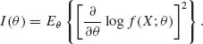
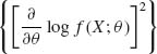
Notice that according to this definition, ![]() log f(x; θ) should exist with probability one, under Fθ, and its second moment should exist. The random variable
log f(x; θ) should exist with probability one, under Fθ, and its second moment should exist. The random variable ![]() log f(x; θ) is called the score function. In Example 3.11 we show a few cases.
log f(x; θ) is called the score function. In Example 3.11 we show a few cases.
We develop now some properties of the Fisher information when the density functions in ![]() satisfy the following set of regularity conditions.
satisfy the following set of regularity conditions.
 < ∞ for each θ
 One can show that under condition (iii) (using the Lebesgue Dominated Convergence Theorem)
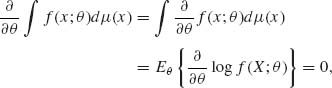
for all θ ![]() Θ. Thus, under these regularity conditions,
Θ. Thus, under these regularity conditions,
![]()
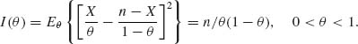
This may not be true if conditions (3.7.2) do not hold. Example 3.11 illustrates such a case where X ∼ R(0, θ). Indeed, if X ∼ R(0, θ) then
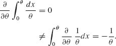
Moreover, in that example Vθ ![]() for all θ. Returning back to cases where regularity conditions (3.7.2) are satisfied, we find that if X1, …, Xn are i.i.d. and In(θ) is the Fisher information function based on their joint distribution,
for all θ. Returning back to cases where regularity conditions (3.7.2) are satisfied, we find that if X1, …, Xn are i.i.d. and In(θ) is the Fisher information function based on their joint distribution,
(3.7.4) 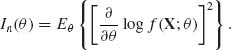
Since X1, …, Xn are i.i.d. random variables, then
(3.7.5) ![]()
and due to (3.7.3),
(3.7.6) ![]()
Thus, under the regularity conditions (3.7.2), I(θ) is an additive function.
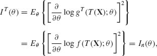
We consider now the information available in a statistic S = (S1(X), …, Sr(X)), where 1 ≤ r ≤ n. Let gS(y1, …, yr; θ) be the joint p.d.f. of S. The Fisher information function corresponding to S is analogously
(3.7.7) 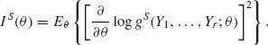
We obviously assume that the family of induced distributions of S satisfies the regularity conditions (i)–(iv). We show now that
We first show that
We prove (3.7.9) first for the discrete case. The general proof follows. Let A(y) = {x; S1(x) = y1, …, Sr(x) = yr}. The joint p.d.f. of S at y is given by
(3.7.10) ![]()
where f(x;θ) is the joint p.d.f. of X. Accordingly,
(3.7.11) 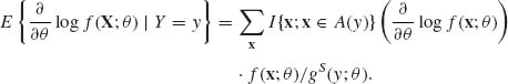
Furthermore, for each x such that f(x; θ ) > 0 and according to regularity condition (iii),
(3.7.12) 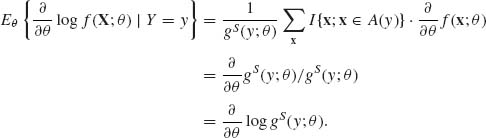
To prove (3.7.9) generally, let S: (![]() ,
, ![]() ,
,![]() ) → (
) → (![]() , Γ,
, Γ, ![]() ) be a statistic and
) be a statistic and ![]()
![]() μ and
μ and ![]() be regular. Then, for any C
be regular. Then, for any C ![]() Γ,
Γ,
(3.7.13) 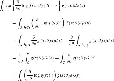
Since C is arbitrary, (3.7.9) is proven. Finally, to prove (3.7.8), write
(3.7.14) 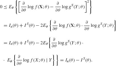
We prove now that if T(X)is a sufficient statistic for ![]() , then
, then
![]()
Indeed, from the Factorization Theorem, if T(X) is sufficient for ![]() then f(x;θ) = K(x) g(T(x); θ), for all θ
then f(x;θ) = K(x) g(T(x); θ), for all θ ![]() Θ. Accordingly, In(θ) = Eθ
Θ. Accordingly, In(θ) = Eθ 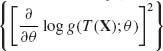 . On the other hand, the p.d.f. of T(X) is gT(t; θ) = A(t)g(t; θ), all θ
 ![]() Θ. Hence,
Θ. Hence, ![]() log gT(t; θ) =
log gT(t; θ) = ![]() log g(t; θ) for all θ and all t. This implies that
log g(t; θ) for all θ and all t. This implies that
for all θ ![]() Θ. Thus, we have proven that if a family of distributions,
Θ. Thus, we have proven that if a family of distributions, ![]() , admits a sufficient statistic, we can determine the amount of information in the sample from the distribution of the m.s.s.
, admits a sufficient statistic, we can determine the amount of information in the sample from the distribution of the m.s.s.
Under regularity conditions (3.7.2), for any statistic U(X),
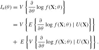
By (3.7.15), if U(X) is an ancillary statistic, log gU(u; θ) is independent of θ. In this case ![]() log gU(u; θ) =
log gU(u; θ) = ![]() , with probability 1, and
, with probability 1, and
![]()
3.7.2 The Kullback–Leibler Information
The Kullback–Leibler (K–L) information function, to discriminate between two distributions Fθ(x) and F![]() (x) of
(x) of ![]() = {Fθ(x); θ
= {Fθ(x); θ ![]() Θ } is defined as
Θ } is defined as
(3.7.16) ![]()
The family ![]() is assumed to be regular. We show now that I(θ,
is assumed to be regular. We show now that I(θ, ![]() ) ≥ 0 with equality if and only if f(X; θ) = f(X;
) ≥ 0 with equality if and only if f(X; θ) = f(X; ![]() ) with probability one. To verify this, we remind that log x is a concave function of x and by the Jensen inequality (see problem 8, Section 2.5), log (E{Y}) ≥ E{log Y} for every nonnegative random variable Y, having a finite expectation. Accordingly,
) with probability one. To verify this, we remind that log x is a concave function of x and by the Jensen inequality (see problem 8, Section 2.5), log (E{Y}) ≥ E{log Y} for every nonnegative random variable Y, having a finite expectation. Accordingly,
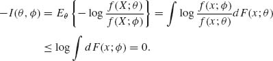
Thus, multiplying both sides of (3.7.17) by −1, we obtain that I(θ, ![]() ) ≥ 0. Obviously, if Pθ {f(X; θ ) = f(X;
) ≥ 0. Obviously, if Pθ {f(X; θ ) = f(X; ![]() )} = 1, then I(θ,
)} = 1, then I(θ, ![]() ) = 0. If X1, …, Xn are i.i.d. random variables, then the information function in the whole sample is
) = 0. If X1, …, Xn are i.i.d. random variables, then the information function in the whole sample is
(3.7.18) 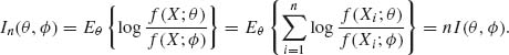
This shows that the K–L information function is additive if the random variables are independent.
If S(X) = (S1(X), …, Sr(X)), 1 ≤ r ≤ n, is a statistic having a p.d.f. gS(y1, …, yr; θ), then the K–L information function based on the information in S(X) is
(3.7.19) ![]()
We show now that
for all θ, ![]()
![]() Θ and every statistic S(X) with equality if S(X) is a sufficient statistic. Since the logarithmic function is concave, we obtain from the Jensen inequality
Θ and every statistic S(X) with equality if S(X) is a sufficient statistic. Since the logarithmic function is concave, we obtain from the Jensen inequality
Generally, if S is a statistic,
![]()
then for any C ![]() Γ
Γ
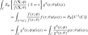
This proves that
(3.7.22) ![]()
Substituting this expression for the conditional expectation in (3.7.21) and multiplying both sides of the inequality by −1, we obtain (3.7.20). To show that if S(X) is sufficient then equality holds in (3.7.20), we apply the Factorization Theorem. Accordingly, if S(X) is sufficient for ![]() ,
,
(3.7.23) ![]()
at all points x at which K(x) > 0. We recall that this set is independent of θ and has probability 1. Furthermore, the p.d.f. of S(X) is
(3.7.24) ![]()
Therefore,
(3.7.25) 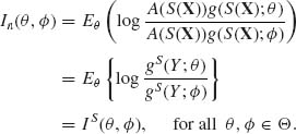
3.8 THE FISHER INFORMATION MATRIX
We generalize here the notion of the information for cases where f(x; θ) depends on a vector of k–parameters. The score function, in the multiparameter case, is defined as the random vector
Under the regularity conditions (3.7.2), which are imposed on each component of θ,
(3.8.2) ![]()
The covariance matrix of S(θ ;X) is the Fisher Information Matrix (FIM)
(3.8.3) ![]()
If the components of (3.8.1) are not linearly dependent, then I(θ) is positive definite.
In the k–parameter canonical exponential type family
(3.8.4) ![]()
The score vector is then
(3.8.5) ![]()
and the FIM is
(3.8.6) 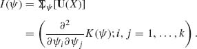
Thus, in the canonical exponential type family, I(![]() ) is the Hessian matrix of the cumulant generating function K(
) is the Hessian matrix of the cumulant generating function K(![]() ).
).
It is interesting to study the effect of reparametrization on the FIM. Suppose that the original parameter vector is θ. We reparametrize by defining the k functions
![]()
Let
![]()
and
![]()
Then,
![]()
It follows that the FIM, in terms of the parameters w, is
Notice that I(![]() (w)) is obtained from I(θ) by substituting
(w)) is obtained from I(θ) by substituting ![]() (w) for θ.
(w) for θ.
Partition θ into subvectors θ(1), …, θ(l) (2 ≤ l ≤ k). We say that θ(1), …, θ(l) are orthogonal subvectors if the FIM is block diagonal, with l blocks, each containing only the parameters in the corresponding subvector.
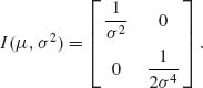
In Example 3.14, μ and σ2 are orthogonal parameters, while ![]() 1 and
1 and ![]() 2 are not orthogonal.
2 are not orthogonal.
3.9 SENSITIVITY TO CHANGES IN PARAMETERS
3.9.1 The Hellinger Distance
There are a variety of distance functions for probability functions. Following Pitman (1979), we apply here the Hellinger distance.
Let ![]() = {F(x; θ), θ
= {F(x; θ), θ ![]() Θ } be a family of distribution functions, dominated by a σ–finite measure μ, i.e., dF(x; θ ) = f(x; θ )dμ (x), for all θ
Θ } be a family of distribution functions, dominated by a σ–finite measure μ, i.e., dF(x; θ ) = f(x; θ )dμ (x), for all θ ![]() Θ. Let θ1, θ2 be two points in Θ. The Hellinger distance between f(x; θ1) and f(x;θ2) is
Θ. Let θ1, θ2 be two points in Θ. The Hellinger distance between f(x; θ1) and f(x;θ2) is
(3.9.1) ![]()
Obviously, ρ (θ1, θ2) = 0 if θ1 = θ2.
Notice that
(3.9.2) ![]()
Thus, ρ(θ1, θ2) ≤ ![]() , for all θ1, θ2
, for all θ1, θ2 ![]() Θ.
Θ.
The sensitivity of ρ(θ1, θ0) at θ0 is the derivative (if it exists) of ρ(θ, θ0), at θ = θ0.
Notice that
If one can introduce the limit, as θ → θ0, under the integral at the r.h.s. of (3.9.3), then
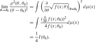
Thus, if the regularity conditions (3.7.2) are satisfied, then
Equation (3.9.5) expresses the sensitivity of ρ(θ, θ0), at θ0, as a function of the Fisher information I(θ0).
Families of densities that do not satisfy the regularity conditions (3.7.2) usually will not satisfy (3.9.5). For example, consider the family of rectangular distributions ![]() = {R(0, θ), 0 < θ < ∞ }.
= {R(0, θ), 0 < θ < ∞ }.
For θ > θ0 > 0,
Thus,
![]()
On the other hand, according to (3.7.1) with n = 1, ![]() .
.
The results of this section are generalizable to families depending on k parameters (θ1, …, θk). Under similar smoothness conditions, if λ = (λ1, …, λk)′ is such that λ′λ = 1, then
(3.9.6) ![]()
where I(θ0) is the FIM.
PART II: EXAMPLES
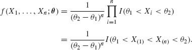
Example 3.1. Let X1, …, Xn be i.i.d. random variables having an absolutely continuous distribution with a p.d.f. f(x). Here we consider the family ![]() of all absolutely continuous distributions. Let T(X) = (X(1), …, X(n)), where X(1) ≤ ··· ≤ X(n), be the order statistic. It is immediately shown that
of all absolutely continuous distributions. Let T(X) = (X(1), …, X(n)), where X(1) ≤ ··· ≤ X(n), be the order statistic. It is immediately shown that
![]()
Thus, the order statistic is a sufficient statistic. This result is obvious because the order at which the observations are obtained is irrelevant to the model. The order statistic is always a sufficient statistic, when the random variables are i.i.d. On the other hand, as will be shown in the sequel, any statistic that further reduces the data is insufficient for ![]() and causes some loss of information.
and causes some loss of information. ![]()
Example 3.2. Let X1, …, Xn be i.i.d. random variables having a Poisson distribution, P(λ). The family under consideration is ![]() = {P(λ); 0 < λ < ∞ }. Let T(X) =
= {P(λ); 0 < λ < ∞ }. Let T(X) = ![]() . We know that T(X) ∼ P(n λ). Furthermore, the joint p.d.f. of X and T(X) is
. We know that T(X) ∼ P(n λ). Furthermore, the joint p.d.f. of X and T(X) is
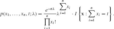
Hence, the conditional p.d.f. of X given T(X) = t is
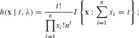
where x1, …, xn are nonnegative integers and t = 0, 1, …. We see that the conditional p.d.f. of X given T(X) = t is independent of λ. Hence T(X) is a sufficient statistic. Notice that X1, …, Xn have a conditional multinomial distribution given Σ Xi = t. ![]()
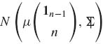
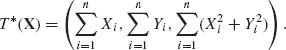
Example 3.3. Let X = (X1, …, Xn)′ have a multinormal distribution N(μ 1n, In), where 1n = (1, 1, …, 1)′. Let ![]() . We set X* = (X2, …, Xn) and derive the joint distribution of (X*, T). According to Section 2.9, (X*, T) has the multinormal distribution
. We set X* = (X2, …, Xn) and derive the joint distribution of (X*, T). According to Section 2.9, (X*, T) has the multinormal distribution
where
Hence, the conditional distribution of X* given T is the multinormal
![]()
where ![]() is the sample mean and Vn−1 = In−1 −
is the sample mean and Vn−1 = In−1 − ![]() Jn−1. It is easy to verify that Vn−1 is nonsingular. This conditional distribution is independent of μ. Finally, the conditional p.d.f. of X1 given (X*, T) is that of a one–point distribution
Jn−1. It is easy to verify that Vn−1 is nonsingular. This conditional distribution is independent of μ. Finally, the conditional p.d.f. of X1 given (X*, T) is that of a one–point distribution
![]()
We notice that it is independent of μ. Hence the p.d.f. of X given T is independent of μ and T is a sufficient statistic. ![]()
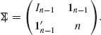
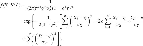
Example 3.4. Let (X1, Y1), …, (Xn, Yn) be i.i.d. random vectors having a bivariate normal distribution. The joint p.d.f. of the n vectors is
where −-∞ < ξ, η < ∞; 0 < σ1, σ2 < ∞; −1 ≤ ρ ≤ 1. This joint p.d.f. can be written in the form
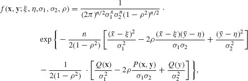
where ![]() ,
, ![]() ,
, ![]() ,
, ![]() , P(x, y) =
, P(x, y) = ![]() (xi −
(xi − ![]() )(yi −
)(yi − ![]() ).
).
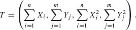
According to the Factorization Theorem, a sufficient statistic for ![]() is
is
![]()
It is interesting that even if σ1 and σ2 are known, the sufficient statistic is still T(X, Y). On the other hand, if ρ = 0 then the sufficient statistic is T*(X, Y) = (![]() ,
, ![]() , Q(X), Q(Y)).
, Q(X), Q(Y)). ![]()
Example 3.5.
A. Binomial Distributions
![]() = {B(n, θ), 0 < θ < 1}, n is known. X1, …, Xn is a sample of i.i.d. random variables. For every point x0, at which f(x0, θ) > 0, we have
= {B(n, θ), 0 < θ < 1}, n is known. X1, …, Xn is a sample of i.i.d. random variables. For every point x0, at which f(x0, θ) > 0, we have
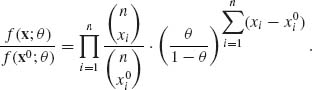
Accordingly, this likelihood ratio can be independent of θ if and only if ![]() . Thus, the m.s.s. is T(X) =
. Thus, the m.s.s. is T(X) = ![]() .
.
B. Hypergeometric Distributions
Xi ∼ H(N, M, S), i = 1, …, n. The joint p.d.f. of the sample is
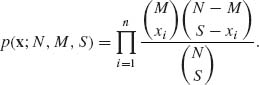
The unknown parameter here is M, M = 0, …, N. N and S are fixed known values. The minimal sufficient statistic is the order statistic Tn = (X(1), …, X(n)). To realize it, we consider the likelihood ratio
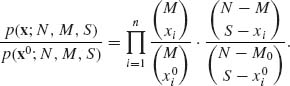
This ratio is independent of (M) if and only if x(i) = ![]() , for all i = 1, 2, …, n.
, for all i = 1, 2, …, n.
C. Negative–Binomial Distributions
Xi ∼ NB(![]() , ν), i = 1, …, n; 0 <
, ν), i = 1, …, n; 0 < ![]() < 1, 0 < ν < ∞.
< 1, 0 < ν < ∞.
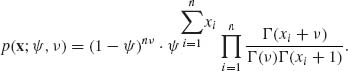
Therefore, the m.s.s. is ![]() .
.
![]()
Hence, the minimal sufficient statistic is the order statistic.
D. Multinomial Distributions
We have a sample of n i.i.d. random vectors![]() , i = 1, …, n. Each X(i) is distributed like the multinomial M(s, θ). The joint p.d.f. of the sample is
, i = 1, …, n. Each X(i) is distributed like the multinomial M(s, θ). The joint p.d.f. of the sample is
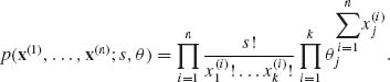
Accordingly, an m.s.s. is ![]() , where
, where ![]() , j = 1, …, k − 1. Notice that
, j = 1, …, k − 1. Notice that 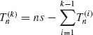 .
.
E. Beta Distributions
![]()
The joint p.d.f. of the sample is
![]()
0 ≤ xi ≤ 1 for all i = 1, …, n. Hence, an m.s.s. is 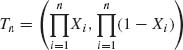 . In cases where either p or q are known, the m.s.s. reduces to the component of Tn that corresponds to the unknown parameter.
F. Gamma Distributions
![]()
The joint distribution of the sample is
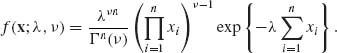
Thus, if both λ and ν are unknown, then an m.s.s. is  . If only ν is unknown, the m.s.s. is
 ![]() . If only λ is unknown, the corresponding statistic
. If only λ is unknown, the corresponding statistic ![]() is minimal sufficient.
is minimal sufficient.
G. Weibull Distributions
X has a Weibull distribution if (X −ξ)α ∼ E(λ). This is a three–parameter family, θ = (ξ, λ, α); where ξ is a location parameter (the density is zero for all x < ξ); λ−1 is a scale parameter; and α is a shape parameter. We distinguish among three cases.
Let Yi = Xi − ξ, i = 1, …, n. Since ![]() ∼ E(λ), we immediately obtain from that an m.s.s., which is,
∼ E(λ), we immediately obtain from that an m.s.s., which is,
![]()
The joint p.d.f. of the sample is
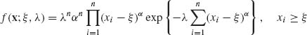
for all i = 1, …, n. By examining this joint p.d.f., we realize that a minimal sufficient statistic is the order statistic, i.e., Tn = (X(1), …, X(n)).
H. Extreme Value Distributions
The joint p.d.f. of the sample is
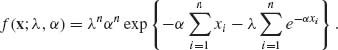
Hence, if α is known then ![]() is a minimal sufficient statistic; otherwise, a minimal sufficient statistic is the order statistic.
is a minimal sufficient statistic; otherwise, a minimal sufficient statistic is the order statistic.
Normal Distributions
![]()
The m.s.s. is 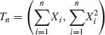 . If ξ is known, then an m.s.s. is
 ![]() ; if σ is known, then the first component of Tn is sufficient.
; if σ is known, then the first component of Tn is sufficient.
We consider a two–sample model according to which X1, …, Xn are i.i.d. having a N(ξ, ![]() ) distribution and Y1, …, Ym are i.i.d. having a N(η,
) distribution and Y1, …, Ym are i.i.d. having a N(η, ![]() ) distribution. The X–sample is independent of the Y–sample. In the general case, an m.s.s. is
) distribution. The X–sample is independent of the Y–sample. In the general case, an m.s.s. is
If ![]() =
= ![]() then the m.s.s. reduces to
then the m.s.s. reduces to 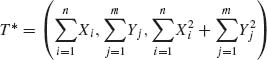 . On the other hand, if ξ = η but σ1 ≠ σ2 then the minimal statistic is T.
 ![]()
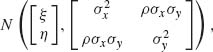
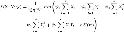
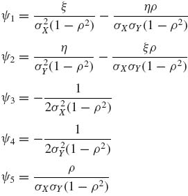
Example 3.6. Let (X, Y) have a bivariate distribution ![]() ,
, ![]() with −∞ < ξ1, ξ2 < ∞; 0 < σ1, σ2 < ∞. The p.d.f. of (X, Y) is
with −∞ < ξ1, ξ2 < ∞; 0 < σ1, σ2 < ∞. The p.d.f. of (X, Y) is
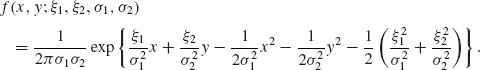
This bivariate p.d.f. can be written in the canonical form
![]()
where
![]()
and
![]()
Thus, if ![]() 1,
1, ![]() 2,
2, ![]() 3, and
3, and ![]() 4 are independent, then an m.s.s. is T(X) =
4 are independent, then an m.s.s. is T(X) = 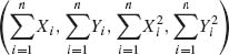 . This is obviously the case when ξ1, ξ2, σ1, σ2 can assume arbitrary values. Notice that if ξ1 = ξ2 but σ1 ≠ σ2 then
 ![]() 1, …,
1, …, ![]() 4 are still independent and T(X) is an m.s.s. On the other hand, if ξ1 ≠ ξ2 but σ1 = σ2 then an m.s.s. is
4 are still independent and T(X) is an m.s.s. On the other hand, if ξ1 ≠ ξ2 but σ1 = σ2 then an m.s.s. is
The case of ξ1 =ξ2, σ1 ≠ σ2, is a case of four–dimensional m.s.s., when the parameter space is three–dimensional. This is a case of a curved exponential family. ![]()
Example 3.7. Binomial Distributions
![]() = {B(n, θ); 0 < θ < 1}, n fixed. Suppose that Eθ {h(X)} = 0 for all 0 < θ < 1. This implies that
= {B(n, θ); 0 < θ < 1}, n fixed. Suppose that Eθ {h(X)} = 0 for all 0 < θ < 1. This implies that
0 < ![]() < ∞, where
< ∞, where ![]() = θ/(1 − θ) is the odds ratio. Let an, j =
= θ/(1 − θ) is the odds ratio. Let an, j = ![]() , j = 0, …, n. The expected value of h(X) is a polynomial of order n in
, j = 0, …, n. The expected value of h(X) is a polynomial of order n in ![]() . According to the fundamental theorem of algebra, such a polynomial can have at most n roots. However, the hypothesis is that the expected value is zero for all
. According to the fundamental theorem of algebra, such a polynomial can have at most n roots. However, the hypothesis is that the expected value is zero for all ![]() in (0, ∞ ). Hence an, j = 0 for all j = 0, …, n, independently of
in (0, ∞ ). Hence an, j = 0 for all j = 0, …, n, independently of ![]() . Or,
. Or,
![]()
![]()
Example 3.8. Rectangular Distributions
Suppose that ![]() = {R(0, θ); 0 < θ < ∞ }. Let X1, …, Xn be i.i.d. random variables having a common distribution from
= {R(0, θ); 0 < θ < ∞ }. Let X1, …, Xn be i.i.d. random variables having a common distribution from ![]() . Let X(n) be the sample maximum. We show that the family of distributions of X(n),
. Let X(n) be the sample maximum. We show that the family of distributions of X(n), ![]() , is complete. The p.d.f. of X(n) is
, is complete. The p.d.f. of X(n) is
![]()
Suppose that Eθ {h(X(n))} = 0 for all 0 < θ < ∞. That is
![]()
Consider this integral as a Lebesque integral. Differentiating with respect to θ yields
![]()
θ ![]() (0, ∞ ).
(0, ∞ ). ![]()
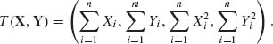
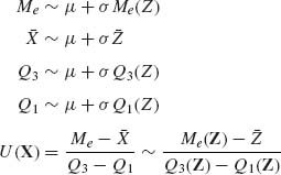
Example 3.9. In Example 2.15, we considered the Model II of analysis of variance. The complete sufficient statistic for that model is
![]()
where ![]() is the grand mean;
is the grand mean; 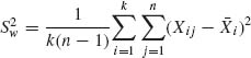 is the “within” sample variance; and
 ![]() is the “between” sample variance. Employing Basu’s Theorem we can immediately conclude that
is the “between” sample variance. Employing Basu’s Theorem we can immediately conclude that ![]() is independent of (
is independent of (![]() ,
, ![]() ). Indeed, if we consider the subfamily
). Indeed, if we consider the subfamily ![]() σ, ρ for a fixed σ and ρ, then
σ, ρ for a fixed σ and ρ, then ![]() is a complete sufficient statistic. The distributions of
is a complete sufficient statistic. The distributions of ![]() and
and ![]() , however, do not depend on μ. Hence, they are independent of
, however, do not depend on μ. Hence, they are independent of ![]() . Since this holds for any σ and ρ, we obtain the result.
. Since this holds for any σ and ρ, we obtain the result. ![]()
Example 3.10. This example follows Example 2.23 of Barndorff–Nielsen and Cox (1994, p. 42). Consider the random vector N = (N1, N2, N3, N4) having a multinomial distribution M(n, p) where p = (p1, …, p4)′ and, for 0 < θ < 1,
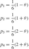
The distribution of N is a curved exponential type. N is an m.s.s., but N is incomplete. Indeed, ![]() for all 0 < θ < 1, but
for all 0 < θ < 1, but ![]() < 1 for all θ. Consider the statistic A1 = N1 + N2. A1 ∼ B
< 1 for all θ. Consider the statistic A1 = N1 + N2. A1 ∼ B ![]() . Thus, A1 is ancillary. The conditional p.d.f. of N, given A1 = a is
. Thus, A1 is ancillary. The conditional p.d.f. of N, given A1 = a is
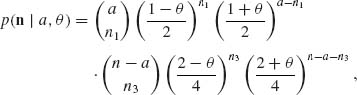
for n1 = 0, 1, …, a; n3 = 0, 1, …, n − a; n2 = a − n1 and n4 = n − a − n3. Thus, N1 is conditionally independent of N3 given A1 = a. ![]()
Example 3.11. A. Let X ∼ B(n, θ), n known, 0 < θ < 1; f(x; θ) = ![]() (1 − θ)n − x satisfies the regularity conditions (3.7.2). Furthermore,
(1 − θ)n − x satisfies the regularity conditions (3.7.2). Furthermore,
![]()
Hence, the Fisher information function is
B. Let X1, …, Xn be i.i.d. random variables having a rectangular distribution R(0, θ), 0 < θ < ∞. The joint p.d.f. is
![]()
where ![]() . Accordingly,
. Accordingly,
![]()
and the Fisher information in the whole sample is
![]()
C. Let X ∼ μ + G(1, 2), −∞ < μ < ∞. In this case,
![]()
Thus,
![]()
But
![]()
Hence, I(μ ) does not exist. ![]()
Example 3.12. In Example 3.10, we considered a four–nomial distribution with parameters pi(θ ), i = 1, …, 4, which depend on a real parameter θ, 0 < θ < 1. We considered two alternative ancillary statistics A = N1 + N2 and A′ = N1 + N4. The question was, which ancillary statistic should be used for conditional inference. Barndorff–Nielsen and Cox (1994, p. 43) recommend to use the ancillary statistic which maximizes the variance of the conditional Fisher information.
A version of the log–likelihood function, conditional on {A = a} is
![]()
This yields the conditional score function
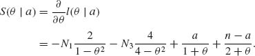
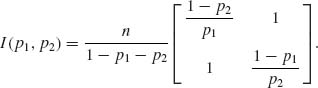
The corresponding conditional Fisher information is
![]()
Finally, since A∼ ![]()
![]() , the Fisher information is
, the Fisher information is
In addition,
![]()
In a similar fashion, we can show that
![]()
and
![]()
Thus, V{I(θ | A)} > V{I(θ | A′)} for all 0 < θ < 1. Ancillary A is preferred. ![]()
Example 3.13. We provide here a few examples of the Kullback–Leibler information function.
A. Normal Distributions
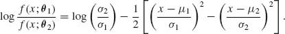
Let ![]() be the class of all the normal distributions {N(μ, σ2); −∞ < μ < ∞, 0 < σ < ∞ }. Let θ1 = (μ1, σ1) and θ2 = (μ2, σ2). We compute I(θ1, θ2). The likelihood ratio is
be the class of all the normal distributions {N(μ, σ2); −∞ < μ < ∞, 0 < σ < ∞ }. Let θ1 = (μ1, σ1) and θ2 = (μ2, σ2). We compute I(θ1, θ2). The likelihood ratio is
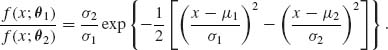
Thus,
Obviously, ![]() . On the other hand
. On the other hand

where U ∼ N (0, 1). Hence, we obtain that
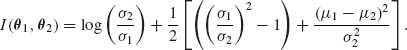
We see that the distance between the means contributes to the K–L information function quadratically while the contribution of the variances is through the ratio ρ = σ2/σ1.
B. Gamma Distributions
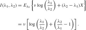
Let θi = (λi, νi), i = 1, 2, and consider the ratio
![]()
We consider here two cases.
Case I: ν1 = ν2 = ν. Since the νs are the same, we simplify by setting θi = λi (i = 1, 2). Accordingly,
This information function depends on the scale parameters λi (i = 1, 2), through their ratio ρ = λ2/λ1.
Case II: λ1 = λ2 = λ. In this case, we write
![]()
Furthermore,
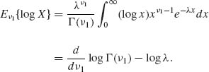
The derivative of the log–gamma function is tabulated (Abramowitz and Stegun, 1968). ![]()
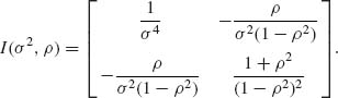
Example 3.14. Consider the normal distribution N(μ, σ2); −∞ < μ < ∞, 0 < σ2 < ∞. The score vector, with respect to θ = (μ, σ2), is
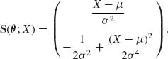
Thus, the FIM is
We have seen in Example 2.16 that this distribution is a two–parameter exponential type, with canonical parameters ![]() 1 =
1 = ![]() and
and ![]() 2 =
2 = ![]() . Making the reparametrization in terms of
. Making the reparametrization in terms of ![]() 1 and
1 and ![]() 2, we compute the FIM as a function of
2, we compute the FIM as a function of ![]() 1,
1, ![]() 2.
2.
The inverse transformation is

Thus,
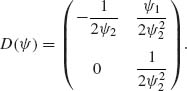
Substituting (3.8.9) into (3.8.8) and applying (3.8.7) we obtain
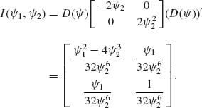
Notice that ![]() .
. ![]()
Example 3.15. Let (X, Y) have the bivariate normal distribution ![]() , 0 < σ2 < ∞, −1 < ρ < 1. This is a two–parameter exponential type family with
, 0 < σ2 < ∞, −1 < ρ < 1. This is a two–parameter exponential type family with
![]()
where U1(x, y) = x2 + y2, U2(x, y) = xy and
![]()
The Hessian of K(![]() 1,
1, ![]() 2) is the FIM, with respect to the canonical parameters. We obtain
2) is the FIM, with respect to the canonical parameters. We obtain
![]()
Using the reparametrization formula, we get
Notice that in this example neither ![]() 1,
1, ![]() 2 nor σ2, ρ are orthogonal parameters.
2 nor σ2, ρ are orthogonal parameters. ![]()
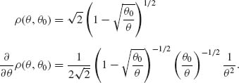
Example 3.16. Let ![]() = {E(λ), 0 < λ < ∞ }. ρ2(λ1, λ2) =
= {E(λ), 0 < λ < ∞ }. ρ2(λ1, λ2) = ![]() . Notice that
. Notice that ![]() for all 0 < λ1, λ2 < ∞. If λ1 = λ2 then ρ (λ1, λ2) = 0. On the other hand, 0 < ρ2 (λ1, λ2) < 2 for all 0 < λ1, λ2 < ∞. However, for λ1 fixed
for all 0 < λ1, λ2 < ∞. If λ1 = λ2 then ρ (λ1, λ2) = 0. On the other hand, 0 < ρ2 (λ1, λ2) < 2 for all 0 < λ1, λ2 < ∞. However, for λ1 fixed
![]()
![]()
PART III: PROBLEMS
Section 3.2
3.2.1 Let X1, …, Xn be i.i.d. random variables having a common rectangular distribution R(θ1, θ2), −∞ < θ1 < θ2 < ∞.
3.2.2 Let X1, X2, …, Xn be i.i.d. random variables having a two–parameter exponential distribution, i.e., X ∼ μ + E(λ), −∞ < μ < ∞, 0 < λ < ∞. Let X(1) ≤ ··· ≤ Xn be the order statistic.
3.2.3 Consider the linear regression model (Problem 3, Section 2.9). The unknown parameters are (α, β, σ). What is a sufficient statistic for ![]() ?
?
3.2.4 Let X1, …, Xn be i.i.d. random variables having a Laplace distribution with p.d.f.
![]()
0 < σ < ∞. What is a sufficient statistic for ![]()
Section 3.3
3.3.1 Let X1, …, Xn be i.i.d. random variables having a common Cauchy distribution with p.d.f.
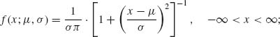
−∞ < μ < ∞, 0 < σ < ∞. What is an m.s.s. for ![]() ?
?
3.3.2 Let X1, …, Xn be i.i.d. random variables with a distribution belonging to a family ![]() of contaminated normal distributions, having p.d.f.s,
of contaminated normal distributions, having p.d.f.s,
−∞ < μ < ∞; 0 < σ < ∞; 0 < α < 10−2. What is an m.s.s. for ![]() ?
?
3.3.3 Let X1, …, Xn be i.i.d. having a common distribution belonging to the family ![]() of all location and scale parameter beta distributions, having the p.d.f.s
of all location and scale parameter beta distributions, having the p.d.f.s
![]()
−μ ≤ x ≤ μ + σ; −∞ < μ < ∞; 0 < σ < ∞; 0 < p, q < ∞.
3.3.4 Let X1, …, Xn be i.i.d. random variables having a rectangular R(θ1, θ2), −∞ < θ1 < θ2 < ∞. What is an m.s.s.?
3.3.5 ![]() is a family of joint distributions of (X, Y) with p.d.f.s
is a family of joint distributions of (X, Y) with p.d.f.s
![]()
Given a sample of n i.i.d. random vectors (Xi, Yi), i = 1, …, n, what is an m.s.s. for ![]() ?
?
3.3.6 The following is a model in population genetics, called the Hardy–Weinberg model. The frequencies N1, N2, N3, ![]() = n, of three genotypes among n individuals have a distribution belonging to the family
= n, of three genotypes among n individuals have a distribution belonging to the family ![]() of trinomial distributions with parameters (n, p1(θ), p2(θ ), p3(θ)), where
of trinomial distributions with parameters (n, p1(θ), p2(θ ), p3(θ)), where
(3.3.1) ![]()
0 < θ < 1. What is an m.s.s. for ![]() ?
?
Section 3.4
3.4.1 Let X1, …, Xn be i.i.d. random variables having a common distribution with p.d.f.
![]()
−∞ < ![]() 1 <
1 < ![]() 2 < ∞. Prove that T(X) =
2 < ∞. Prove that T(X) = 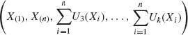 is an m.s.s.
3.4.2 Let {(Xk, Yi), i = 1, …, n} be i.i.d. random vectors having a common bivariate normal distribution
where −∞ < ξ, η < ∞; 0 < ![]() ,
, ![]() < ∞; −1 < ρ < 1.
< ∞; −1 < ρ < 1.
3.4.3 In continuation of the previous problem, what is the m.s.s.
Section 3.5
3.5.1 Let ![]() = {Gα (λ, 1); 0 < α < ∞, 0 < λ < ∞ } be the family of Weibull distributions. Is
= {Gα (λ, 1); 0 < α < ∞, 0 < λ < ∞ } be the family of Weibull distributions. Is ![]() complete?
complete?
3.5.2 Let ![]() be the family of extreme–values distributions. Is
be the family of extreme–values distributions. Is ![]() complete?
complete?
3.5.3 Let ![]() = {R(θ1, θ2); −∞ < θ1 < θ2 < ∞ }. Let X1, X2, …, Xn, n ≥ 2, be a random sample from a distribution of
= {R(θ1, θ2); −∞ < θ1 < θ2 < ∞ }. Let X1, X2, …, Xn, n ≥ 2, be a random sample from a distribution of ![]() . Is the m.s.s. complete?
. Is the m.s.s. complete?
3.5.4 Is the family of trinomial distributions complete?
3.5.5 Show that for the Hardy–Weinberg model the m.s.s. is complete.
Section 3.6
3.6.1 Let {(Xi, Yi), i = 1, …, n} be i.i.d. random vectors distributed like ![]() , −1 < ρ < 1.
, −1 < ρ < 1.
3.6.2 Let X1, …, Xn be i.i.d. random variables having a normal distribution N(μ, σ2), where both μ and σ are unknown.
Section 3.7
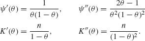
3.7.1 Consider the one–parameter exponential family with p.d.f.s
![]()
Show that the Fisher information function for θ is
![]()
Check this result specifically for the Binomial, Poisson, and Negative–Binomial distributions.
3.7.2 Let (Xi, Yi), i = 1, …, n be i.i.d. vectors having the bivariate standard normal distribution with unknown coefficient of correlation ρ, −1 ≤ ρ ≤ 1. Derive the Fisher information function In(ρ).
3.7.3 Let ![]() (x) denote the p.d.f. of N(0, 1). Define the family of mixtures
(x) denote the p.d.f. of N(0, 1). Define the family of mixtures
![]()
Derive the Fisher information function I(α).
3.7.4 Let ![]() = {f(x;
= {f(x; ![]() ), −∞ <
), −∞ < ![]() < ∞ } be a one–parameter exponential family, where the canonical p.d.f. is
< ∞ } be a one–parameter exponential family, where the canonical p.d.f. is
![]()
![]()
3.7.5 Let X1, …, Xn be i.i.d. N(0, σ2), 0 < σ2 < ∞.
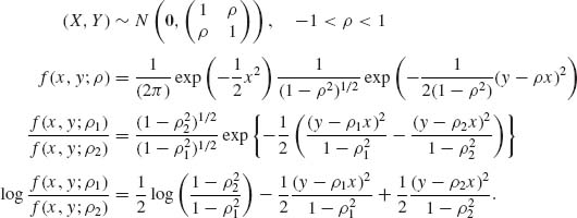
3.7.6 Let (X, Y) have the bivariate standard normal distribution ![]() , −1 < ρ < 1. X is an ancillary statistic. Derive the conditional Fisher information I(ρ | X) and then the Fisher information I(ρ ).
, −1 < ρ < 1. X is an ancillary statistic. Derive the conditional Fisher information I(ρ | X) and then the Fisher information I(ρ ).
3.7.7 Consider the model of Problem 6. What is the Kullback–Leibler information function I(ρ1, ρ2) for discriminating between ρ1 and ρ2 where −1 ≤ ρ1 < ρ2 ≤ 1.
3.7.8 Let X ∼ P(λ). Derive the Kullback–Leibler information I(λ1, λ2) for 0 < λ1, λ2 < ∞.
3.7.9 Let X ∼ B(n, θ). Derive the Kullback–Liebler information function I(θ1, θ2), 0 < θ1, θ2 < 1.
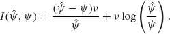
3.7.10 Let X ∼ G(λ, ν), 0 < λ < ∞, ν known.
Section 3.8
3.8.1 Consider the trinomial distribution M(n, p1, p2), 0 < p1, p2, p1 + p2 < 1.
![]()
3.8.2 Consider the bivariate normal distribution. Derive the FIM I(ξ, η, σ1, σ2, ρ).
3.8.3 Consider the gamma distribution G(λ, ν). Derive the FIM I(λ, ν).
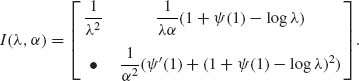
3.8.4 Consider the Weibull distribution W(λ, α) ∼ (G(λ, 1))1/2; 0 < α, λ < ∞. Derive the Fisher informaton matrix I(λ, α).
Section 3.9
3.9.1 Find the Hellinger distance between two Poisson distributions with parameters λ1 and λ2.
3.9.2 Find the Hellinger distance between two Binomial distributions with parameters p1≠ p2 and the same parameter n.
3.9.3 Show that for the Poisson and the Binomial distributions Equation (3.9.4) holds.
PART IV: SOLUTIONS TO SELECTED PROBLEMS
3.2.1 X1, …, Xn are i.i.d. ∼ R(θ1, θ2), 0 < θ1 < θ2 < ∞.
Thus, f(X1, …, Xn; θ) = A(x)g(T(x), θ), where A(x) = 1 ![]() x and
x and
![]()
T(X) = (X(1), X(n)) is a likelihood statistic and thus minimal sufficient.
![]()
Let (X(1), …, X(n)) be the order statistic. The p.d.f. of (X(1), …, X(n)) is
![]()
The conditional p.d.f. of (X(1), …, X(n)) given (X(1), X(n)) is
![]()
That is, (X(2), …, X(n−1)) given (X(1), X(n)) are distributed like the (n − 2) order statistic of (n − 2) i.i.d. from R(X(1), X(n)).
3.3.6 The likelihood function of θ, 0 < θ < 1, is
![]()
Since N3 = n − N1 − N2, 2N3 + N2 = 2n − 2N1 − N2. Hence,
![]()
The sample size n is known. Thus, the m.s.s. is Tn = 2N1 + N2.
3.4.1
The likelihood function of ![]() is
is
Thus 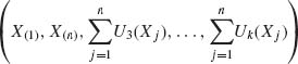 is a likelihood statistic, i.e., minimal sufficient.
3.4.2 The joint p.d.f. of (Xi, Yi), i = 1, …, n is
In canonical form, the joint density is
where
and
![]()
The m.s.s. for ![]() is T(X, Y) = (Σ Xi, Σ Yi, Σ
is T(X, Y) = (Σ Xi, Σ Yi, Σ ![]() , Σ
, Σ ![]() , Σ XiYi).
, Σ XiYi).
3.5.5 We have seen that the likelihood of θ is L(θ) ![]() θT(N)(1 − θ)2n − T(N) where T(N) = 2N1 + N2. This is the m.s.s. Thus, the distribution of T(N) is B(2n, θ). Finally
θT(N)(1 − θ)2n − T(N) where T(N) = 2N1 + N2. This is the m.s.s. Thus, the distribution of T(N) is B(2n, θ). Finally ![]() = B(2n, θ), 0 < θ < 1} is complete.
= B(2n, θ), 0 < θ < 1} is complete.
3.6.2
independent of μ and σ.
3.7.1 The score function is
![]()
Hence, the Fisher information is
![]()
Consider the equation
![]()
Differentiating both sides of this equation with respect to θ, we obtain that
![]()
Differentiating the above equations twice with respect to θ, yields
![]()
Thus, we get
![]()
Therefore
![]()
In the Binomial case,
![]()
Thus, ![]() (θ) = log
(θ) = log ![]() , K(θ) = −n log (1 − θ)
, K(θ) = −n log (1 − θ)
Hence, I(θ) = ![]() .
.
In the Poisson case,
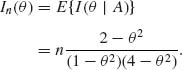
8 In the Negative–Binomial case, ν known,
![]()
3.7.2 Let ![]() .
.
Let l(ρ) denote the log–likelihood function of ρ, −1 < ρ < 1. This is
![]()
Furthermore,
![]()
Recall that I(ρ) = E{−l″(ρ)}. Moreover,
![]()
Thus,
![]()
3.7.7
Thus, the Kullback–Leibler information is
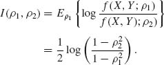
The formula is good also for ρ1 > ρ2.
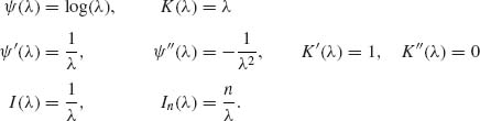
3.7.10 The p.d.f. of G(λ, ν) is
![]()
When ν is known, we can write the p.d.f. as g(x; ![]() ) = h(x) exp (
) = h(x) exp (![]() x + ν log (−
x + ν log (−![]() )), where h(x) =
)), where h(x) = ![]() ,
, ![]() = −λ. The value of
= −λ. The value of ![]() maximizing g(x,
maximizing g(x, ![]() ) is
) is ![]() = −
= −![]() . The K–L information I(
. The K–L information I(![]() 1,
1, ![]() ) is
) is
![]()
Substituting ![]() 1 =
1 = ![]() , we have
, we have
Thus,

3.8.2 The log–likelihood function is
The score coefficients are
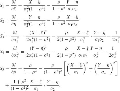
The FIM
![]()
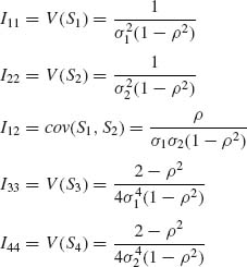
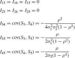
and
![]()
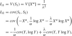
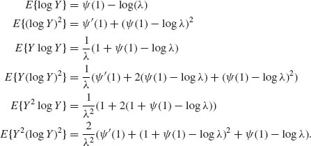
3.8.4 The FIM for the Weibull parameters. The likelihood function is
![]()
Thus,
![]()
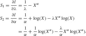
Recall that Xα ∼ E(λ). Thus, E{Xα} = ![]() and E{S1} = 0. Let
and E{S1} = 0. Let ![]() (1) denote the di-gamma function at 1 (see Abramowitz and Stegun, 1965, pp. 259). Then,
(1) denote the di-gamma function at 1 (see Abramowitz and Stegun, 1965, pp. 259). Then,
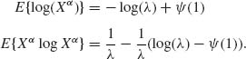
Thus,
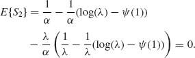
where Y ∼ Xα ∼ E(λ).
Accordingly,
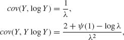
and
![]()
Finally,
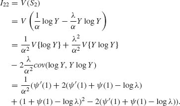
Thus,
![]()
The Fisher Information Matix is