
CHAPTER 4
Testing Statistical Hypotheses
PART I: THEORY
4.1 THE GENERAL FRAMEWORK
Statistical hypotheses are statements about the unknown characteristics of the distributions of observed random variables. The first step in testing statistical hypotheses is to formulate a statistical model that can represent the empirical phenomenon being studied and identify the subfamily of distributions corresponding to the hypothesis under consideration. The statistical model specifies the family of distributions relevant to the problem. Classical tests of significance, of the type that will be presented in the following sections, test whether the deviations of observed sample statistics from the values of the corresponding parameters, as specified by the hypotheses, cannot be ascribed just to randomness. Significant deviations lead to weakening of the hypotheses or to their rejection. This testing of the significance of deviations is generally done by constructing a test statistic based on the sample values, deriving the sampling distribution of the test statistic according to the model and the values of the parameters specified by the hypothesis, and rejecting the hypothesis if the observed value of the test statistic lies in an improbable region under the hypothesis. For example, if deviations from the hypothesis lead to large values of a nonnegative test statistic T(X), we compute the probability that future samples of the type drawn will yield values of T(X) at least as large as the presently observed one. Thus, if we observe the value t0 of T(X), we compute the tail probability
![]()
This value is called the observed significance level or the P–value of the test. A small value of the observed significant level means either that an improbable event has occurred or that the sample data are incompatible with the hypothesis being tested. If α (t0) is very small, it is customary to reject the hypothesis.
One of the theoretical difficulties with this testing approach is that it does not provide a framework for choosing the test statistic. Generally, our intuition and knowledge of the problem will yield a reasonable test statistic. However, the formulation of one hypothesis is insufficient for answering the question whether the proposed test is a good one and how large should the sample be. In order to construct an optimal test, in a sense that will be discussed later, we have to formulate an alternative hypothesis, against the hypothesis under consideration. For distinguishing between the hypothesis and its alternative (which is also a hypothesis), we call the first one a null hypothesis (denoted by H0) and the other one an alternative hypothesis H1. The alternative hypothesis can also be formulated in terms of a subfamily of distributions according to the specified model. We denote this subfamily by ![]() 1. If the family
1. If the family ![]() 0 or
0 or ![]() 1 contains only one element, the corresponding null or alternative hypothesis is called simple, otherwise it is called composite. The null hypothesis and the alternative one enable us to determine not only the optimal test, but also the sample size required to obtain a test having a certain strength. We distinguish between two kinds of errors. An error of Type I is the error due to rejection of the null hypothesis when it is true. An error of Type II is the one committed when the null hypothesis is not rejected when it is false. It is generally impossible to guarantee that a test will never commit either one of the two kinds of errors. A trivial test that always accepts the null hypothesis never commits an error of the first kind but commits an error of the second kind whenever the alternative hypothesis is true. Such a test is powerless. The theoretical framework developed here measures the risk in these two kinds of errors by the probabilities that a certain test will commit these errors. Ideally, the probabilities of the two kinds of errors should be kept low. This can be done by choosing the proper test and by observing a sufficiently large sample. In order to further develop these ideas we introduce now the notion of a test function.
1 contains only one element, the corresponding null or alternative hypothesis is called simple, otherwise it is called composite. The null hypothesis and the alternative one enable us to determine not only the optimal test, but also the sample size required to obtain a test having a certain strength. We distinguish between two kinds of errors. An error of Type I is the error due to rejection of the null hypothesis when it is true. An error of Type II is the one committed when the null hypothesis is not rejected when it is false. It is generally impossible to guarantee that a test will never commit either one of the two kinds of errors. A trivial test that always accepts the null hypothesis never commits an error of the first kind but commits an error of the second kind whenever the alternative hypothesis is true. Such a test is powerless. The theoretical framework developed here measures the risk in these two kinds of errors by the probabilities that a certain test will commit these errors. Ideally, the probabilities of the two kinds of errors should be kept low. This can be done by choosing the proper test and by observing a sufficiently large sample. In order to further develop these ideas we introduce now the notion of a test function.
Let X = (X1, …, Xn) be a vector of random variables observable for the purpose of testing the hypothesis H0 against H1. A function ![]() (X) that assumes values in the interval [0, 1] and is a sample statistic is called a test function. Using a test function
(X) that assumes values in the interval [0, 1] and is a sample statistic is called a test function. Using a test function ![]() (X) and observing X = x, the null hypothesis H0 is rejected with probability
(X) and observing X = x, the null hypothesis H0 is rejected with probability ![]() (x). This is actually a conditional probability of rejecting H0, given {X = x}. For a given value of
(x). This is actually a conditional probability of rejecting H0, given {X = x}. For a given value of ![]() (x), we draw a value R from a table of random numbers, having a rectangular distribution R(0, 1) and reject H0 if R ≤
(x), we draw a value R from a table of random numbers, having a rectangular distribution R(0, 1) and reject H0 if R ≤ ![]() (x). Such a procedure is called a randomized test. If
(x). Such a procedure is called a randomized test. If ![]() (x) is either 0 or 1, for all x, we call the procedure a nonrandomized test. The set of x values in the sample space
(x) is either 0 or 1, for all x, we call the procedure a nonrandomized test. The set of x values in the sample space ![]() for which
for which ![]() (x) = 1 is called the rejection region corresponding to
(x) = 1 is called the rejection region corresponding to ![]() (x).
(x).
We distinguish between test functions according to their size and power. The size of a test function ![]() (x) is the maximal probability of error of the first kind, over all the distribution functions F in
(x) is the maximal probability of error of the first kind, over all the distribution functions F in ![]() 0, i. e., α = sup {E{
0, i. e., α = sup {E{![]() (x)| F }: F
(x)| F }: F ![]()
![]() 0} where E{
0} where E{![]() (x)| F} denotes the expected value of
(x)| F} denotes the expected value of ![]() (x) (the total probability of rejecting H0) under the distribution F. We denote the size of the test by α. The power of a test is the probability of rejecting H0 when the parent distribution F belongs to
(x) (the total probability of rejecting H0) under the distribution F. We denote the size of the test by α. The power of a test is the probability of rejecting H0 when the parent distribution F belongs to ![]() 1. As we vary F over
1. As we vary F over ![]() 1, we can consider the power of a test as a functional
1, we can consider the power of a test as a functional ![]() (F;
(F; ![]() ) over
) over ![]() 1. In parametric cases, where each F can be represented by a real or vector valued parameter θ, we speak about a power function
1. In parametric cases, where each F can be represented by a real or vector valued parameter θ, we speak about a power function ![]() (θ ;
(θ ;![]() ), θ
), θ ![]() Θ1, where Θ1 is the set of all parameter points corresponding to
Θ1, where Θ1 is the set of all parameter points corresponding to ![]() 1. A test function
1. A test function ![]() 0(x) that maximizes the power, with respect to all test functions
0(x) that maximizes the power, with respect to all test functions ![]() (x) having the same size, at every point θ, is called uniformly most powerful (UMP) of size α. Such a test function is optimal. As will be shown, uniformly most powerful tests exist only in special situations. Generally we need to seek tests with some other good properties. Notice that if the model specifies a family of distributions
(x) having the same size, at every point θ, is called uniformly most powerful (UMP) of size α. Such a test function is optimal. As will be shown, uniformly most powerful tests exist only in special situations. Generally we need to seek tests with some other good properties. Notice that if the model specifies a family of distributions ![]() that admits a (nontrivial) sufficient statistic, T(X), then for any specified test function,
that admits a (nontrivial) sufficient statistic, T(X), then for any specified test function, ![]() (x) say, the test function
(x) say, the test function ![]() (T) = E{
(T) = E{![]() (x)| T} is equivalent, in the sense that it has the same size and the same power function. Thus, one can restrict attention only to test functions that depend on minimal sufficient statistics.
(x)| T} is equivalent, in the sense that it has the same size and the same power function. Thus, one can restrict attention only to test functions that depend on minimal sufficient statistics.
The literature on testing statistical hypotheses is so rich that there is no point to try and list here even the important papers. The exposition of the basic theory on various levels of sophistication can be found in almost all the textbooks available on Probability and Mathematical Statistics. For an introduction to the asymptotic (large sample) theory of testing hypotheses, see Cox and Hinkley (1974). More sophisticated discussion of the theory is given in Chapter III of Schmetterer (1974). In the following sections we present an exposition of important techniques. A comprehensive treatment of the theory of optimal tests is given in Lehmann (1997).
4.2 THE NEYMAN–PEARSON FUNDAMENTAL LEMMA
In this section we develop the most powerful test of two simple hypotheses. Thus, let ![]() = {F0, F1} be a family of two specified distribution functions. Let f0(x) and f1(x) be the probability density functions (p. d. f. s) corresponding to the elements of
= {F0, F1} be a family of two specified distribution functions. Let f0(x) and f1(x) be the probability density functions (p. d. f. s) corresponding to the elements of ![]() . The null hypothesis H0 is that the parent distribution is F0. The alternative hypothesis H1 is that the parent distribution is F1. We exclude the problem of testing H0 at size α = 0 since this is obtained by the trivial test function that accepts H0 with probability one (according to F0). The following lemma, which is the basic result of the whole theory, was given by Neyman and Pearson (1933).
. The null hypothesis H0 is that the parent distribution is F0. The alternative hypothesis H1 is that the parent distribution is F1. We exclude the problem of testing H0 at size α = 0 since this is obtained by the trivial test function that accepts H0 with probability one (according to F0). The following lemma, which is the basic result of the whole theory, was given by Neyman and Pearson (1933).
Theorem 4.2.1 (The Neyman–Pearson Lemma) For testing H0 against H1,
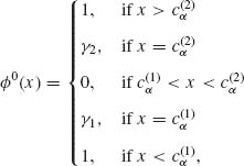
(a) Any test function of the form
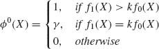
for some 0 ≤ k < ∞ and 0 ≤ γ ≤ 1 is most powerful relative to all tests of its size.
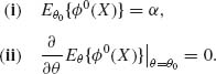
(b) (Existence) For testing H0 against H1, at a level of significance α there exist constants kα, 0 ≤ kα < ∞ and γα, 0 ≤ γα ≤ 1 such that the corresponding test function of the form (4.2.1) is most powerful of size α.
(c) (Uniqueness) If a test ![]() ′ is most powerful of size α, then it is of the form (4.2.1), except perhaps on the set {x;f1(x) = kf0(x)}, unless there exists a test of size smaller than α and power 1.
′ is most powerful of size α, then it is of the form (4.2.1), except perhaps on the set {x;f1(x) = kf0(x)}, unless there exists a test of size smaller than α and power 1.
Proof. (a) Let α be the size of the test function ![]() 0(X) given by (4.2.1). Let
0(X) given by (4.2.1). Let ![]() 1(x) be any other test function whose size does not exceed α, i. e.,
1(x) be any other test function whose size does not exceed α, i. e.,
The expectation in (4.2.2) is with respect to the distribution F0. We show now that the power of ![]() 1(X) cannot exceed that of
1(X) cannot exceed that of ![]() 0(X). Define the sets
0(X). Define the sets
(4.2.3) 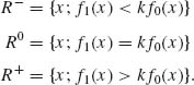
We notice that {R−, R0, R+} is a partition of χ. We prove now that
(4.2.4) ![]()
Indeed,
(4.2.5) 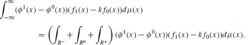
Moreover, since on R− the inequality f1(x) − kf0(x) < 0 is satisfied and ![]() 0(x) = 0, we have
0(x) = 0, we have
Similarly,
(4.2.7) ![]()
and since on R+ ![]() 0(x) = 1,
0(x) = 1,
Hence, from (4.2.6)–(4.2.8) we obtain
The inequality on the RHS of (4.2.9) follows from the assumption that the size of ![]() 0(x) is exactly α and that of
0(x) is exactly α and that of ![]() 1(x) does not exceed α. Hence, from (4.2.9),
1(x) does not exceed α. Hence, from (4.2.9),
(4.2.10) ![]()
This proves (a).
(b) (Existence). Consider the distribution W(ξ) of the random variable f1(X)/f0(X), which is induced by the distribution F0, i. e.,
(4.2.11) ![]()
We notice that P0{f0(X) = 0} = 0. Accordingly W(ξ) is a c. d. f. The γ–quantile of W(ξ) is defined as
(4.2.12) ![]()
For a given value of α, 0 < α < 1, we should determine 0 ≤ kα < ∞ and 0 ≤ γα ≤ 1 so that, according to (4.2.1),
where W(kα) − W(kα −0) is the height of the jump of W(ξ) at kα. Thus, let
(4.2.14) ![]()
Obviously, 0 < kα < ∞, since W(ξ) is a c. d. f. of a nonnegative random variable. Notice that, for a given 0 < α < 1, kα = 0 whenever
![]()
If W(kα) − W(kα − 0) = 0 then define γα = 0. Otherwise, let γα be the unique solution of (4.2.13), i. e.,
Obviously, 0 ≤ γα ≤ 1.
(c) (Uniqueness). For a given α, let ![]() 0(X) be a test function of the form (4.2.1) with kα and γα as in (4.2.15). Suppose that
0(X) be a test function of the form (4.2.1) with kα and γα as in (4.2.15). Suppose that ![]() 1(X) is the most powerful test function of size α. From (4.2.9), we have
1(X) is the most powerful test function of size α. From (4.2.9), we have
But,
(4.2.17) ![]()
and since ![]() 0 is most powerful,
0 is most powerful,
![]()
Hence, (4.2.16) equals to zero. Moreover, the integrand on the LHS of (4.2.16) is nonnegative. Therefore, it must be zero for all x except perhaps on the union of R0 and a set N of probability zero. It follows that on (R+ − N) ![]() (R− − N),
(R− − N), ![]() 0(x) =
0(x) = ![]() 1(x). On the other hand, if
1(x). On the other hand, if ![]() 1(x) has size less than α and power 1, then the above argument is invalid. QED
1(x) has size less than α and power 1, then the above argument is invalid. QED
An extension of the Neyman–Pearson Fundamental Lemma to cases of testing m hypotheses H1, …, Hm against an alternative Hm+1 was provided by Chernoff and Scheffé (1952). This generalization provides a most powerful test of Hm+1 under the constraint that the Type I error probabilities of H1, …, Hm do not exceed α1, …, αm, correspondingly where 0 < αi < 1, i = 1, …, m. See also Dantzig and Wald (1951).
4.3 TESTING ONE–SIDED COMPOSITE HYPOTHESES IN MLR MODELS
In this section we show that the most powerful tests, which are derived according to the Neyman–Pearson Lemma, can be uniformly most powerful for testing composite hypotheses in certain models. In the following example we illustrate such a case.
A family of distributions ![]() = {F(x;θ), θ
= {F(x;θ), θ ![]() Θ }, where Θ is an interval on the real line, is said to have the monotone likelihood ratio property (MLR) if, for every θ1 < θ2 in Θ, the likelihood ratio
Θ }, where Θ is an interval on the real line, is said to have the monotone likelihood ratio property (MLR) if, for every θ1 < θ2 in Θ, the likelihood ratio
![]()
is a nondecreasing function of x. We also say that ![]() is an MLR family with respect to X. For example, consider the one–parameter exponential type family with p. d. f.
is an MLR family with respect to X. For example, consider the one–parameter exponential type family with p. d. f.
![]()
This family is MLR with respect to U(X).
The following important lemma was proven by Karlin (1956).
Theorem 4.3.1 (Karlin’s Lemma) Suppose that ![]() = {F(x;θ);−∞ < θ < ∞ } is an MLR family w. r. t. x. If g(x) is a nondecreasing function of x, then Eθ {g(X)} is a nondecreasing function of θ. Furthermore, for any θ < θ′, F(x;θ) ≥ F(x;θ′) for all x.
= {F(x;θ);−∞ < θ < ∞ } is an MLR family w. r. t. x. If g(x) is a nondecreasing function of x, then Eθ {g(X)} is a nondecreasing function of θ. Furthermore, for any θ < θ′, F(x;θ) ≥ F(x;θ′) for all x.
Proof. (i) Consider two points θ, θ′ such that θ < θ′. Define the sets
(4.3.1) ![]()
where f(x;θ) are the corresponding p. d. f. s. Since f(x;θ′) /f(x;θ) is a nondecreasing function of x, if x ![]() A and x ′
A and x ′ ![]() B then x < x′. Therefore,
B then x < x′. Therefore,
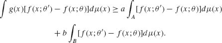
We wish to show that Eθ′{g(X)} ≥ Eθ {g(X)}. Consider,
(4.3.3) 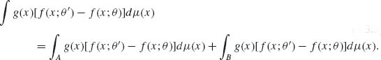
Furthermore, since on the set A f(x;θ′) − f(x;θ) < 0, we have
(4.3.4) ![]()
Hence,
Moreover, for each ![]() ,
,
![]()
In particular,
(4.3.6) 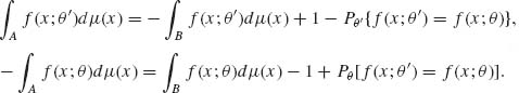
This implies that
Moreover, from (4.3.5) and (4.3.7), we obtain that
(4.3.8) ![]()
Indeed, from (4.3.2), (b−a) ≥ 0 and according to the definition of B, ![]() [f(x;θ′) − f(x;θ)]dμ (x) ≥ 0. This completes the proof of part (i).
[f(x;θ′) − f(x;θ)]dμ (x) ≥ 0. This completes the proof of part (i).
(ii) For any given x, define ![]() x(y) = I{y;y > x}.
x(y) = I{y;y > x}. ![]() x(y) is a nondecreasing function of y. According to part (i) if θ′ > θ then Eθ {
x(y) is a nondecreasing function of y. According to part (i) if θ′ > θ then Eθ {![]() x(Y)} ≤ Eθ′{
x(Y)} ≤ Eθ′{![]() x(Y)}. We notice that Eθ {
x(Y)}. We notice that Eθ {![]() x(Y)} = Pθ {Y > x} = 1 − F(x;θ). Thus, if θ < θ′ then F(x;θ) ≥ F(x;θ′) for all x. QED
x(Y)} = Pθ {Y > x} = 1 − F(x;θ). Thus, if θ < θ′ then F(x;θ) ≥ F(x;θ′) for all x. QED
Theorem 4.3.2 If a one–parameter family ![]() = {Fθ (x); −∞ < θ < ∞ } admits a sufficient statistic T(X) and if the corresponding family of distributions of T(X),
= {Fθ (x); −∞ < θ < ∞ } admits a sufficient statistic T(X) and if the corresponding family of distributions of T(X), ![]() T, is MLR with respect to T(X), then the test function
T, is MLR with respect to T(X), then the test function
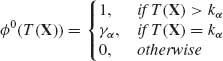
has the following properties.
Proof. For simplicity of notation we let T(x) = x (real).
(i) From the Neyman–Pearson Lemma, a most powerful test of ![]() : θ = θ0 against
: θ = θ0 against ![]() : θ = θ1, θ1 > θ0 is of the form
: θ = θ1, θ1 > θ0 is of the form
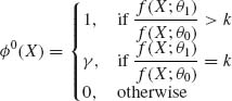
provided 0 ≤ k < ∞. Hence, since ![]() is an MLR w. r. t. X, f(X;θ1)/f(X;θ0) > k implies that X > x0. x0 is determined from the equation f(x0;θ1)/f(x0;θ0) = k. Thus, (4.3.9) is also most powerful for testing
is an MLR w. r. t. X, f(X;θ1)/f(X;θ0) > k implies that X > x0. x0 is determined from the equation f(x0;θ1)/f(x0;θ0) = k. Thus, (4.3.9) is also most powerful for testing ![]() against
against ![]() at the same size as (4.3.10). The constants x0 and γ are determined so that (4.3.9) and (4.3.10) will have the same size. Thus, if α is the size of (4.3.10) then x0 and γ should satisfy the equation
at the same size as (4.3.10). The constants x0 and γ are determined so that (4.3.9) and (4.3.10) will have the same size. Thus, if α is the size of (4.3.10) then x0 and γ should satisfy the equation
(4.3.11) ![]()
Hence, x0 and γ may depend only on θ0, but are independent of θ1. Therefore, the test function ![]() 0(X) given by (4.3.9) is uniformly most powerful for testing
0(X) given by (4.3.9) is uniformly most powerful for testing ![]() against H0. Moreover, since
against H0. Moreover, since ![]() 0(X) is a nondecreasing function of X, the size of the test
0(X) is a nondecreasing function of X, the size of the test ![]() 0 (for testing H0 against H1) is α. Indeed, from Karlin’s Lemma the power function
0 (for testing H0 against H1) is α. Indeed, from Karlin’s Lemma the power function ![]() (θ ;
(θ ;![]() 0) = Eθ {
0) = Eθ {![]() 0(X)} is a nondecreasing function of θ (which proves (iii)). Hence,
0(X)} is a nondecreasing function of θ (which proves (iii)). Hence, ![]() Eθ {
Eθ {![]() 0(X)} = α. Thus,
0(X)} = α. Thus, ![]() 0(X) is uniformly most powerful for testing H0 against H1.
0(X) is uniformly most powerful for testing H0 against H1.
(ii) The proof of this part is simple. Given any α, 0 < α < 1, we set x0 = F−1(1 − α;θ0) where F−1(γ, θ) denotes the γ–quantile of F(x;θ). If F(x;θ0) is continuous at x0, we set γ = 0, otherwise
(4.3.12) ![]() QED
QED
4.4 TESTING TWO–SIDED HYPOTHESES IN ONE–PARAMETER EXPONENTIAL FAMILIES
Consider again the one–parameter exponential type family with p. d. f. s
![]()
A two–sided simple hypothesis is H0: θ = θ0, −∞ < θ0 < ∞. We consider H0 against a composite alternative H1: θ ≠ θ0.
If X = (X1, …, Xn)′ is a vector of independent and identically distributed (i. i. d.) random variables, then the test is based on the minimal sufficient statistic (m. s. s.) T(X) = ![]() U(Xi). The distribution of T(X), for any θ, is also a one–parameter exponential type. Hence, without loss of generality, we present the theory of this section under the simplified notation T(X) = X. We are seeking a test function
U(Xi). The distribution of T(X), for any θ, is also a one–parameter exponential type. Hence, without loss of generality, we present the theory of this section under the simplified notation T(X) = X. We are seeking a test function ![]() 0(X) that will have a power function, which is attaining its minimum at θ = θ0 and Eθ0{
0(X) that will have a power function, which is attaining its minimum at θ = θ0 and Eθ0{![]() 0 (X)} = α, for some preassigned level of significance α, 0 < α < 1. We consider the class of two–sided test functions
0 (X)} = α, for some preassigned level of significance α, 0 < α < 1. We consider the class of two–sided test functions
where ![]() <
< ![]() . Moreover, we determine the values of
. Moreover, we determine the values of ![]() , γ1,
, γ1, ![]() , γ2 by considering the requirement
, γ2 by considering the requirement
Assume that γ1 = γ2 = 0. Then
(4.4.3) ![]()
Moreover,
(4.4.4) ![]()
Thus,
(4.4.5) ![]()
It follows that condition (ii) of (4.4.2) is equivalent to
It is easy also to check that
(4.4.7) ![]()
Since this is a positive quantity, the power function assumes its minimum value at θ = θ0, provided ![]() 0(X) is determined so that (4.4.2) (i) and (4.4.6) are satisfied. As will be discussed in the next section, the two–sided test functions developed in this section are called unbiased.
0(X) is determined so that (4.4.2) (i) and (4.4.6) are satisfied. As will be discussed in the next section, the two–sided test functions developed in this section are called unbiased.
When the family ![]() is not of the one–parameter exponential type, UMP unbiased tests may not exist. For examples of such cases, see Jogdio and Bohrer (1973).
is not of the one–parameter exponential type, UMP unbiased tests may not exist. For examples of such cases, see Jogdio and Bohrer (1973).
4.5 TESTING COMPOSITE HYPOTHESES WITH NUISANCE PARAMETERS—UNBIASED TESTS
In the previous section, we discussed the theory of testing composite hypotheses when the distributions in the family under consideration depend on one real parameter. In this section, we develop the theory of most powerful unbiased tests of composite hypotheses. The distributions under consideration depend on several real parameters and the hypotheses state certain conditions on some of the parameters. The theory that is developed in this section is applicable only if the families of distributions under consideration have certain structural properties that are connected with sufficiency. The multiparameter exponential type families possess this property and, therefore, the theory is quite useful. First development of the theory was attained by Neyman and Pearson (1933, 1936a, 1936b). See also Lehmann and Scheffé (1950, 1955) and Sverdrup (1953).
Definition 4.5.1. Consider a family of distributions, ![]() = {F(x;θ);θ
= {F(x;θ);θ ![]() Θ}, where θ is either real or vector valued. Suppose that the null hypothesis is H0: θ
Θ}, where θ is either real or vector valued. Suppose that the null hypothesis is H0: θ ![]() Θ0 and the alternative hypothesis is H1: θ
Θ0 and the alternative hypothesis is H1: θ ![]() Θ1. A test function
Θ1. A test function ![]() (X) is called unbiased of sizeα if
(X) is called unbiased of sizeα if
![]()
and
(4.5.1) ![]()
In other words, a test function of size α is unbiased if the power of the test is not smaller than α whenever the parent distribution belongs to the family corresponding to the alternative hypothesis. Obviously, the trivial test ![]() (X) = α with probability one is unbiased, since Eθ {
(X) = α with probability one is unbiased, since Eθ {![]() (X)} = α for all θ
(X)} = α for all θ ![]() Θ1. Thus, unbiasedness in itself is insufficient. However, under certain conditions we can determine uniformly most powerful tests among the unbiased ones. Let Θ* be the common boundary of the parametric sets Θ0 and Θ1 corresponding to H0 and H1 respectively. More formally, if
Θ1. Thus, unbiasedness in itself is insufficient. However, under certain conditions we can determine uniformly most powerful tests among the unbiased ones. Let Θ* be the common boundary of the parametric sets Θ0 and Θ1 corresponding to H0 and H1 respectively. More formally, if ![]() 0 is the closure of Θ0 (the union of the set with its limit points) and
0 is the closure of Θ0 (the union of the set with its limit points) and ![]() 1 is the closure of Θ1, then Θ* =
1 is the closure of Θ1, then Θ* = ![]() 0
0 ![]()
![]() 1. For example, if θ = (θ1, θ2), Θ0 = {θ ;θ1 ≤ 0} and Θ1 = {θ ;θ1 > 0}, then Θ* = { θ ;θ1 = 0}. This is the θ2–axis. In testing two–sided hypotheses, H0:
1. For example, if θ = (θ1, θ2), Θ0 = {θ ;θ1 ≤ 0} and Θ1 = {θ ;θ1 > 0}, then Θ* = { θ ;θ1 = 0}. This is the θ2–axis. In testing two–sided hypotheses, H0: ![]() ≤ θ1 ≤
≤ θ1 ≤ ![]() (θ2 arbitrary) against H1: θ1 <
(θ2 arbitrary) against H1: θ1 < ![]() or θ1 >
or θ1 > ![]() (θ2 arbitrary), the boundary consists of the two parallel lines Θ = {θ: θ1 =
(θ2 arbitrary), the boundary consists of the two parallel lines Θ = {θ: θ1 = ![]() or θ1 =
or θ1 = ![]() }.
}.
Definition 4.5.2. For testing H0: θ ![]() Θ0 against H1: θ
Θ0 against H1: θ ![]() Θ1, a test
Θ1, a test ![]() (x) is called α–similar if Eθ {θ (X)} = α for all θ
(x) is called α–similar if Eθ {θ (X)} = α for all θ ![]() Θ0. It is called α– similar on the boundary1 if Eθ {
Θ0. It is called α– similar on the boundary1 if Eθ {![]() (X)} = α for all θ
(X)} = α for all θ ![]() Θ .
Θ .
Let ![]() * denote the subfamily of
* denote the subfamily of ![]() , which consists of all the distributions F(x;θ) where θ belongs to the boundary Θ*, between Θ0 and Θ1. Suppose that
, which consists of all the distributions F(x;θ) where θ belongs to the boundary Θ*, between Θ0 and Θ1. Suppose that ![]() * is such that a nontrivial sufficient statistic T(X) with respect to
* is such that a nontrivial sufficient statistic T(X) with respect to ![]() * exists. In this case, E{
* exists. In this case, E{![]() (X| T(X)} is independent of those θ that belong to the boundary Θ* . That is, this conditional expectation may depend on the boundary, but does not change its value when θ changes over Θ*. If a test
(X| T(X)} is independent of those θ that belong to the boundary Θ* . That is, this conditional expectation may depend on the boundary, but does not change its value when θ changes over Θ*. If a test ![]() (X) has the property that
(X) has the property that
then ![]() (X) is a boundary α–similar test. If a test
(X) is a boundary α–similar test. If a test ![]() (x) satisfies (4.5.2), we say that it has the Neyman structure. If the power function of an unbiased test function
(x) satisfies (4.5.2), we say that it has the Neyman structure. If the power function of an unbiased test function ![]() (x) of size α is a continuous function of θ (θ may be vector valued), then
(x) of size α is a continuous function of θ (θ may be vector valued), then ![]() (x) is a boundary α–similar test function. Furthermore, if the family of distribution of T(X) on the boundary is boundedly complete, then every boundary α–similar test function has the Neyman structure. Indeed, since
(x) is a boundary α–similar test function. Furthermore, if the family of distribution of T(X) on the boundary is boundedly complete, then every boundary α–similar test function has the Neyman structure. Indeed, since ![]() is boundedly complete and since every test function is bounded, Eθ {
is boundedly complete and since every test function is bounded, Eθ {![]() (X)} = α for all θ
(X)} = α for all θ ![]() Θ implies that E{
Θ implies that E{![]() (X)| T(X)} = α with probability 1 for all θ in Θ*. It follows that if the power function of every unbiased test is continuous in θ, then the class of all test functions having the Neyman structure with some α, 0 < α < 1, contains all the unbiased tests of size α. Thus, if we can find a UMP test among those having the Neyman structure and if the test is unbiased, then it is UMP unbiased. This result can be applied immediately in cases of the k–parameter exponential type families. Express the joint p. d. f. of X in the form
(X)| T(X)} = α with probability 1 for all θ in Θ*. It follows that if the power function of every unbiased test is continuous in θ, then the class of all test functions having the Neyman structure with some α, 0 < α < 1, contains all the unbiased tests of size α. Thus, if we can find a UMP test among those having the Neyman structure and if the test is unbiased, then it is UMP unbiased. This result can be applied immediately in cases of the k–parameter exponential type families. Express the joint p. d. f. of X in the form
(4.5.3) 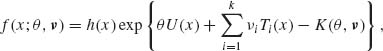
where ν = (ν1, …, νk)′ is a vector of nuisance parameters and θ is real valued. We consider the following composite hypotheses.
![]()
against
![]()
![]()
against
![]()
For the one–sided hypotheses, the boundary is
![]()
For the two–sided hypotheses, the boundary is
![]()
In both cases, the sufficient statistic w. r. t. ![]() * is
* is
![]()
We can restrict attention to test functions ![]() (U, T) since (U, T) is a sufficient statistic for
(U, T) since (U, T) is a sufficient statistic for ![]() . The marginal p. d. f. of T is of the exponential type and is given by
. The marginal p. d. f. of T is of the exponential type and is given by
(4.5.4) 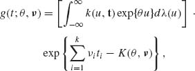
where k(u, t) = ∫ I{x: U(x) = u, I(x) = t} h(x)dμ (x). Hence, the conditional p. d. f. of U given T is a one–parameter exponential type of the form
According to the results of the previous section, we construct uniformly most powerful test functions based on the family of conditional distributions, with p. d. f. s (4.5.5). Accordingly, if the hypotheses are one–sided, we construct the conditional test function
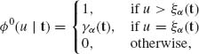
where ξα (t) and γα (t) are determined so that
(4.5.7) ![]()
for all t. We notice that since T(X) is sufficient for ![]() *, γα (t) and ξα (t) can be determined independently of ν. Thus, the test function
*, γα (t) and ξα (t) can be determined independently of ν. Thus, the test function ![]() 0(U| T) has the Neyman structure. It is a uniformly most powerful test among all tests having the Neyman structure.
0(U| T) has the Neyman structure. It is a uniformly most powerful test among all tests having the Neyman structure.
In the two–sided case, we construct the conditional test function
(4.5.8) 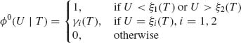
where ξ1(T), ξ2(T), γ1(T), and γ2(T) are determined so that
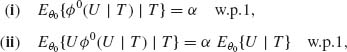
![]()
with probability one. As shown in the previous section, if in the two–sided case θ1 = θ2 = θ0, then we determine γi(T) and ξi(T) (i = 1, 2) so that
where w. p. 1 means “with probability one. ” The test functions ![]() 0(U | T) are uniformly most powerful unbiased ones.
0(U | T) are uniformly most powerful unbiased ones.
The theory of optimal unbiased test functions is strongly reinforced with the following results. Consider first the one–sided hypotheses H0: θ < θ0, ν arbitrary; against H1: θ > θ0, ν arbitrary. We show that if there exists function W(U, T) that is increasing in U for each T (U is real valued) and such that W(U, T) and T are independent under H0, then the test function
(4.5.10) 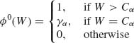
is uniformly most powerful unbiased, where Cα and γα are determined so that the size of ![]() 0(W) is α. Indeed, the power of
0(W) is α. Indeed, the power of ![]() 0(W) at (θ0, ν) is α by construction. Thus,
0(W) at (θ0, ν) is α by construction. Thus,
(4.5.11) ![]()
Since W(U, T) is independent of T at (θ0, ν), Cα and γα are independent of T. Furthermore, since W(U, T) is an increasing function of U for each T, the test function ![]() 0 is equivalent to the conditional test function (4.5.6). Similarly, for testing the two–sided hypotheses H0: θ1 ≤ θ ≤ θ2, ν arbitrary, we can employ the equivalent test function
0 is equivalent to the conditional test function (4.5.6). Similarly, for testing the two–sided hypotheses H0: θ1 ≤ θ ≤ θ2, ν arbitrary, we can employ the equivalent test function
(4.5.12) 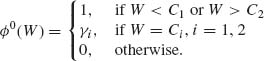
Here, we require that W(U, T) is independent of T at all the points (θ1, ν) and (θ2, ν). When θ1 = θ2 = θ0, we require that W(U, T) = a(T)U + b(T), where a(T) > 0 with probability one. This linear function of U for each T implies that condition (4.5.9) and the condition
(4.5.13) ![]()
are equivalent.
4.6 LIKELIHOOD RATIO TESTS
As defined in Section 3.3, the likelihood function L(θ | x) is a nonnegative function on the parameter space Θ, proportional to the joint p. d. f. f(x;θ). We discuss here tests of composite hypotheses analogous to the Neyman–Pearson likelihood ratio tests. If H0 is a specified null hypothesis, corresponding to the parametric set Θ0 and if Θ is the whole sample space, we define the likelihood ratio statistic as
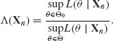
Obviously, 0 ≤ Λ (xn) ≤ 1. A likelihood ratio test is defined as
(4.6.2) ![]()
where Cα is determined so that
(4.6.3) ![]()
Due to the nature of the statistic Λ (Xn), its distribution may be discontinuous at Λ = 1 even if the distribution of Xn is continuous. For this reason, the test may not exist for every α.
Generally, even if a generalized likelihood ratio test of size α exists, it is difficult to determine the critical level Cα. In Example 4.14 we demonstrate such a case. Generally, for parametric models, the sampling distribution of Λ (X), under H0, can be approximated by simulation. In addition, under certain regularity conditions, if H0 is a simple hypotheses and θ is a k–dimensional vector, then the asymptotic distribution of −2 log Λ (Xn) as n→ ∞ is like that of χ2[m], where m = dim (Θ)− dim (Θ0), (Wilks, 1962, Chapter 13, Section 13.4). Thus, if the sample is not too small, the (1−α)–quantile of χ2[m] can provide a good approximation to −2 log Cα. In cases of a composite null hypothesis we have a similar result. However, the asymptotic distribution may not be unique.
4.6.1 Testing in Normal Regression Theory
A normal regression model is one in which n random variables Y1, …, Yn are observed at n different experimental setups (treatment combinations). The vector Yn = (Y1, …, Yn)′ is assumed to have a multinormal distribution N(Xβ, σ2I), where X is an n× p matrix of constants with rank = p and β′ = (β1, …, βp) is a vector of unknown parameters, 1 ≤ p ≤ n. The parameter space is Θ = {(β1, …, βp, σ); −∞ < βi < ∞ for all i = 1, …, p and 0 < σ < ∞ }. Consider the null hypothesis
![]()
where 1 ≤ r < p. Thus, Θ0 = {(β1, …, βr, 0, …, 0, σ); −∞ < βi < ∞ for all i = 1, …, r; 0 < σ < ∞ }. This is the null hypothesis that tests the significance of the (p−r) β–values βj (j = r + 1, …, p). The likelihood function is
![]()
We determine now the values of β and σ for which the likelihood function is maximized, for the given X and Y. Starting with β, we see that the likelihood function is maximized when Q(β) = (Y−Xβ)′(Y −Xβ) is minimized irrespective of σ. The vector β that minimizes Q(β) is called the least–squares estimator of β. Differentiation of Q(β) with respect to the vector β yields
(4.6.4) ![]()
Equating this gradient vector to zero yields the vector
(4.6.5) ![]()
We recall that X′X is nonsingular since X is assumed to be of full rank p. Substituting Q(![]() ) in the likelihood function, we obtain
) in the likelihood function, we obtain
(4.6.6) ![]()
where
(4.6.7) ![]()
and A = I−X(X′X)−1X′ is a symmetric idempotent matrix. Differentiating L(![]() , σ) with respect to σ and equating to zero, we obtain that the value σ2 that maximizes the likelihood function is
, σ) with respect to σ and equating to zero, we obtain that the value σ2 that maximizes the likelihood function is
(4.6.8) ![]()
Thus, the denominator of (4.6.1) is
(4.6.9) ![]()
We determine now the numerator of (4.6.1). Let K = (0:Ip−r) be a (p−r)× p matrix, which is partitioned to a zero matrix of order (p−r)× r and the identity matrix of order (p−r) × (p−r). K is of full rank, and KK′ = Ip−r. The null hypothesis H0 imposes on the linear model the constraint that Kβ = 0. Let β* and ![]() 2 denote the values of β and σ2, which maximize the likelihood function under the constraint Kβ = 0. To determine the value of β*, we differentiate first the Lagrangian
2 denote the values of β and σ2, which maximize the likelihood function under the constraint Kβ = 0. To determine the value of β*, we differentiate first the Lagrangian
(4.6.10) ![]()
where λ is a (p−r) × 1 vector of constants. Differentiating with respect to β, we obtain the simultaneous equations
From (i), we obtain that the constrained least–squares estimator β* is given by
(4.6.12) ![]()
Substituting β* in (4.6.11) (ii), we obtain
(4.6.13) ![]()
Since K is of full rank p−r, K(X′X)−1K′ is nonsingular. Hence,
![]()
and the constrained least–squares estimator is
(4.6.14) ![]()
To obtain σ2, we employ the derivation presented before and find that
(4.6.15) 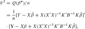
where B = K(X′X)−1K′. Simple algebraic manipulations yield that
(4.6.16) ![]()
Hence, the numerator of (4.6.1) is
(4.6.17) 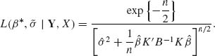
The likelihood ratio is then
(4.6.18) ![]()
This likelihood ratio is smaller than a constant Cα if
is greater than an appropriate constant kα. In this case, we can easily find the exact distribution of the F–ratio (4.6.19). Indeed, according to the results of Section 2.10, Q(![]() ) = Y′AY ~ σ2χ2[n−p] since A = I − X(X′X)−1X′ is an idempotent matrix of rank n−p and since the parameter of noncentrality is
) = Y′AY ~ σ2χ2[n−p] since A = I − X(X′X)−1X′ is an idempotent matrix of rank n−p and since the parameter of noncentrality is
![]()
Furthermore,
(4.6.20) ![]()
Let C = X(X′X)−1K′B−1K(X′X)−1X′. It is easy to verify that C is an idempotent matrix of rank p−r. Hence,
(4.6.21) ![]()
where
(4.6.22) ![]()
We notice that Kβ = (βr+1, …, βp)′, which is equal to zero if the null hypothesis is true. Thus, under H0, λ* = 0 and otherwise, λ* > 0. Finally,
(4.6.23) ![]()
Hence, the two quadratic forms Y′AY and Y′C Y are independent. It follows that under H0, the F ratio (4.6.19) is distributed like a central F[p−r, n−p] statistic, and the critical level kα is the (1−α)–quantile F1−α [p−r, n−p]. The power function of the test is
(4.6.24) ![]()
A special case of testing in normal regression theory is the analysis of variance (ANOVA). We present this analysis in the following section.
4.6.2 Comparison of Normal Means: The Analysis of Variance
Consider an experiment in which r independent samples from normal distributions are observed. The basic assumption is that all the r variances are equal, i. e., σ![]() = ··· =
= ··· = ![]() = σ2 (r ≥ 2). We test the hypothesis H0: μ1 = ··· = μr, σ2 arbitrary. The sample m. s. s. is (
= σ2 (r ≥ 2). We test the hypothesis H0: μ1 = ··· = μr, σ2 arbitrary. The sample m. s. s. is (![]() 1, …,
1, …, ![]() r,
r, ![]() ), where
), where ![]() i is the mean of the ith sample and
i is the mean of the ith sample and ![]() is the pooled “within” variance defined in the following manner. Let ni be the size of the ith sample, νi = ni−1;
is the pooled “within” variance defined in the following manner. Let ni be the size of the ith sample, νi = ni−1; ![]() , the variance of the ith sample; and let ν =
, the variance of the ith sample; and let ν = ![]() νi. Then
νi. Then
(4.6.25) ![]()
Since the sample means are independent of the sample variances in normal distributions, ![]() is independent of
is independent of ![]() 1, …,
1, …, ![]() r. The variance “between” samples is
r. The variance “between” samples is
(4.6.26) ![]()
where ![]() is the grand mean. Obviously
is the grand mean. Obviously ![]() and
and ![]() are independent. Moreover, under H0,
are independent. Moreover, under H0, ![]() ~
~ ![]() and
and ![]() ~
~ ![]() . Hence, the variance ratio
. Hence, the variance ratio
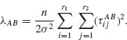
is distributed, under H0, like a central F[r−1, ν] statistic. The hypothesis H0 is rejected if F ≥ F1−α [r−1, ν]. If the null hypothesis H0 is not true, the distribution of ![]() is like that of
is like that of ![]() χ2 [r−1;λ], where the noncentrality parameter is given by
χ2 [r−1;λ], where the noncentrality parameter is given by
and ![]() is a weighted average of the true means. Accordingly, the power of the test, as a function of λ, is
is a weighted average of the true means. Accordingly, the power of the test, as a function of λ, is
This power function can be expressed according to (2.12.22) as
where ξ = F1−α[r−1, ν] and ![]() .
.
4.6.2.1 One–Way Layout Experiments
The F–test given by (4.6.27) is a basic test statistic in the analysis of statistical experiments. The method of analysis is known as a one–way layout analysis of variance (ANOVA). Consider an experiment in which N = n· r experimental units are randomly assigned to r groups (blocks). Each group of n units is then subjected to a different treatment. More specifically, one constructs a statistical model assuming that the observed values in the various groups are samples of independent random variables having normal distributions. Furthermore, it is assumed that all the r normal distributions have the same variance σ2 (unknown). The r means are represented by the linear model
(4.6.31) ![]()
where ![]() = 0. The parameters τ1, …, τr represent the incremental effects of the treatments. μ is the (grand) average yield associated with the experiment. Testing whether the population means are the same is equivalent to testing whether all τi = 0, i = 1, …, r. Thus, the hypotheses are
= 0. The parameters τ1, …, τr represent the incremental effects of the treatments. μ is the (grand) average yield associated with the experiment. Testing whether the population means are the same is equivalent to testing whether all τi = 0, i = 1, …, r. Thus, the hypotheses are
![]()
against
![]()
We perform the F–test (4.6.27). The parameter of noncentrality (4.6.28) assumes the value
(4.6.32) ![]()
4.6.2.2 Two–Way Layout Experiments
If the experiment is designed to test the incremental effects of two factors (drug A and drug B) and their interaction, and if factor A is observed at r1 levels and factor B at r2 levels, there should be s = r1 × r2 groups (blocks) of size n. It is assumed that these s samples are mutually independent, and the observations within each sample represent i. i. d. random variables having N(μij, σ2) distributions, i = 1, …, r1; j = 1, …, r2. The variances are all the same. The linear model is expressed in the form
![]()
where ![]() , and
, and  for each i = 1, …, r1 and
 ![]() = 0 for each j = 1, …, r2. The parameters
= 0 for each j = 1, …, r2. The parameters ![]() are called the main effects of factor A;
are called the main effects of factor A; ![]() are called the main effects of factors B; and
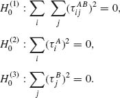
are called the main effects of factors B; and ![]() are the interaction parameters. The hypotheses that one may wish to test are whether the main effects are significant and whether the interaction is significant. Thus, we set up the null hypotheses:
are the interaction parameters. The hypotheses that one may wish to test are whether the main effects are significant and whether the interaction is significant. Thus, we set up the null hypotheses:
These hypotheses are tested by constructing F–tests in the following manner. Let Xijk, i = 1, …, r1; j = 1, …, r2; and k = 1, …, n designate the observed random variable (yield) of the kth unit at the (i, j)th group. Let ![]() ij denote the sample mean of the (i, j)th group;
ij denote the sample mean of the (i, j)th group; ![]() i., the overall mean of the groups subject to level i of factor A;
i., the overall mean of the groups subject to level i of factor A; ![]() · j, the overall mean of the groups subject to level j of factor B; and
· j, the overall mean of the groups subject to level j of factor B; and ![]() , the grand mean; i. e.,
, the grand mean; i. e.,
(4.6.34) 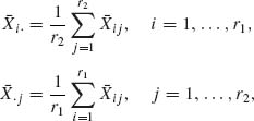
and
![]()
The sum of squares of deviations around ![]() is partitioned into four components in the following manner.
is partitioned into four components in the following manner.
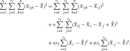
The four terms on the right–hand side of (4.6.35) are mutually independent quadratic forms having distributions proportional to those of central or noncentral chi–squared random variables. Let us denote by Qr the quadratic form on the left–hand side of (4.6.35) and the terms on the right–hand side (moving from left to right) by QW, QAB, QA, and QB, respectively. Then we can show that
(4.6.36) ![]()
Similarly,
(4.6.37) ![]()
and the parameter of noncentrality is
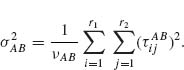
Let ![]() = QW/νW and
= QW/νW and ![]() = QAB/νAB. These are the pooled sample variance within groups and the variance between groups due to interaction. If the null hypothesis
= QAB/νAB. These are the pooled sample variance within groups and the variance between groups due to interaction. If the null hypothesis ![]() of zero interaction is correct, then the F–ratio,
of zero interaction is correct, then the F–ratio,
(4.6.39) ![]()
is distributed like a central F[νAB, νW]. Otherwise, it has a noncentral F–distribution as F[νAB, νW; λAB]. Notice also that
(4.6.40) ![]()
and
(4.6.41) ![]()
where
Formula (4.6.42) can be easily derived from (4.6.38) by employing the mixing relationship (2.8.6), χ2 [νAB;λAB] ~ χ2[νAB + 2J], where J is a Poisson random variable, P(λAB). To test the hypotheses ![]() and
and ![]() , concerning the main effects of A and B, we construct the F–statistics
, concerning the main effects of A and B, we construct the F–statistics
(4.6.43) 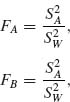
where ![]() = QA/νA, νA = r1 − 1 and
= QA/νA, νA = r1 − 1 and ![]() = QB/νB, νB = r2 − 1. Under the null hypotheses these statistics have central F[νA, νW] and F[νB, νW] distributions. Indeed, for each i = 1, …, r1,
= QB/νB, νB = r2 − 1. Under the null hypotheses these statistics have central F[νA, νW] and F[νB, νW] distributions. Indeed, for each i = 1, …, r1, ![]() i· ~ N(μ +
i· ~ N(μ + ![]() , σ2/nr2). Hence,
, σ2/nr2). Hence,
(4.6.44) ![]()
with
(4.6.45) ![]()
Similarly,
(4.6.46) ![]()
with
(4.6.47) 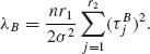
Under the null hypotheses ![]() and
and ![]() both λA and λB are zero. Thus, the (1−α)–quantiles of the central F–distributions mentioned above provide critical values of the test statistics FA and FB. We also remark that
both λA and λB are zero. Thus, the (1−α)–quantiles of the central F–distributions mentioned above provide critical values of the test statistics FA and FB. We also remark that
(4.6.48) 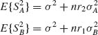
where
(4.6.49) 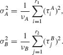
These results are customarily summarized in the following table of ANOVA.
Table 4.1 A Two–Way Scheme for Analysis of Variance
Finally, we would like to remark that the three tests of significance provided by FAB, FA, and FB are not independent, since the within variance estimator ![]() is used by all the three test statistics. Moreover, if we wish that the level of significance of all the three tests simultaneously will not exceed α, we should reduce that of each test to α /3. In other words, suppose that
is used by all the three test statistics. Moreover, if we wish that the level of significance of all the three tests simultaneously will not exceed α, we should reduce that of each test to α /3. In other words, suppose that ![]() ,
, ![]() , and
, and ![]() are true and we wish not to reject either one of these. We accept simultaneously the three hypotheses in the event of {FAB ≤ F1−α /3[νAB, νW], FA ≤ F1−α /3[νA, νB], FB ≤ F1−α /3[νB, νW]}. According to the Bonferroni inequality, if E1, E2, and E3 are any three events
are true and we wish not to reject either one of these. We accept simultaneously the three hypotheses in the event of {FAB ≤ F1−α /3[νAB, νW], FA ≤ F1−α /3[νA, νB], FB ≤ F1−α /3[νB, νW]}. According to the Bonferroni inequality, if E1, E2, and E3 are any three events
(4.6.50) ![]()
where ![]() i (i = 1, 2, 3) designates the complement of Ei. Thus, the probability that all the three hypotheses will be simultaneously accepted, given that they are all true, is at least 1−α. Generally, a scientist will find the result of the analysis very frustrating if all the null hypotheses are accepted. However, by choosing the overall α as sufficiently small, the rejection of any of these hypotheses becomes very meaningful. For further reading on testing in linear models, see Lehmann (1997, Chapter 7), Anderson (1958), Graybill (1961, 1976), Searle (1971) and others.
i (i = 1, 2, 3) designates the complement of Ei. Thus, the probability that all the three hypotheses will be simultaneously accepted, given that they are all true, is at least 1−α. Generally, a scientist will find the result of the analysis very frustrating if all the null hypotheses are accepted. However, by choosing the overall α as sufficiently small, the rejection of any of these hypotheses becomes very meaningful. For further reading on testing in linear models, see Lehmann (1997, Chapter 7), Anderson (1958), Graybill (1961, 1976), Searle (1971) and others.
4.7 THE ANALYSIS OF CONTINGENCY TABLES
4.7.1 The Structure of Multi–Way Contingency Tables and the Statistical Model
There are several qualitative variables A1, …, Ak. The ith variable assumes mi levels (categories). A sample of N statistical units are classified according to the M = ![]() mi combinations of the levels of the k variables. These level combinations will be called cells. Let f(i1, …, ik) denote the observed frequency in the (i1, …, ik) cell. We distinguish between contingency tables having fixed or random marginal frequencies. In this section we discuss only structures with random margins. The statistical model assumes that the vector of M frequencies has a multinomial distribution with parameters N and P, where P is the vector of cell probabilities P(i1, …, ik). We discuss here some methods of testing the significance of the association (dependence) among the categorical variables.
mi combinations of the levels of the k variables. These level combinations will be called cells. Let f(i1, …, ik) denote the observed frequency in the (i1, …, ik) cell. We distinguish between contingency tables having fixed or random marginal frequencies. In this section we discuss only structures with random margins. The statistical model assumes that the vector of M frequencies has a multinomial distribution with parameters N and P, where P is the vector of cell probabilities P(i1, …, ik). We discuss here some methods of testing the significance of the association (dependence) among the categorical variables.
4.7.2 Testing the Significance of Association
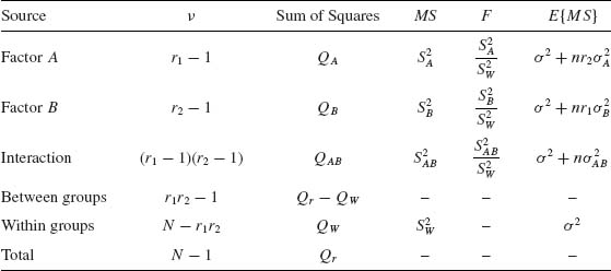
We illustrate the test for association in a two–way table that is schematized below.
Table 4.2 A Scheme of a Two–Way Contingency Table
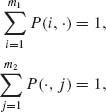
f(i, j) is the observed frequency of the (i, j)th cell. We further denote the observed marginal frequencies by
(4.7.1) 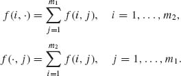
Let
(4.7.2) 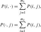
denote the marginal probabilities.
The categorical variables A and B are independent if and only if P(i, j) = P(i, ·)P(·, j) for all (i, j). Thus, if A and B are independent, the expected frequency at (i, j) is
(4.7.3) ![]()
Since P(i, ·) and P(·, j) are unknown, we estimate E(i, j) by
(4.7.4) 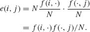
The deviations of the observed frequencies from the expected are tested for randomness by
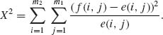
Simple algebraic manipulations yield the statistic
We test the hypothesis of no association by comparing X2 to the (1−α)th quantile of χ2[ν] with ν = (m1−1)(m2−1) degrees of freedom. We say that the association is significant if X2 ≥ ![]() [ν]. This is a large sample test. In small samples it may be invalid. There are appropriate test procedures for small samples, especially for 2× 2 tables. For further details, see Lancaster (1969, Chapters XI, XII).
[ν]. This is a large sample test. In small samples it may be invalid. There are appropriate test procedures for small samples, especially for 2× 2 tables. For further details, see Lancaster (1969, Chapters XI, XII).
4.7.3 The Analysis of 2× 2 Tables
Consider the following 2 × 2 table of cell probabilities
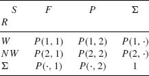
S and R are two variables (success in a course and race, for example). The odds ratio of F/P for W is defined as P(1, 1)/P(1, 2) and for NW it is P(2, 1)/P(2, 2).
These odds ratios are also called the relative risks. We say that there is no interaction between the two variables if the odds ratios are the same. Define the cross product ratio
If ρ = 1 there is no interaction; otherwise, the interaction is negative or positive according to whether ρ < 1 or ρ > 1, respectively. Alternatively, we can measure the interaction by
(4.7.8) ![]()
We develop now a test of the significance of the interaction, which is valid for any sample size and is a uniformly most powerful test among the unbiased tests.
Consider first the conditional joint distribution of X = f(1, 1) and Y = f(2, 1) given the marginal frequency T = f(1, 1) + f(1, 2). It is easy to prove that conditional on T, X and Y are independent and have conditional binomial distributions B(T, P(1, 1)/P(1, ·)) and B(N−T, P(2, 1)/P(2, ·)), respectively. We consider now the conditional distribution of X given the marginal frequencies T = f(1, ·) and S = f(1, 1) + f(2, 1) = f(·, 1). This conditional distribution has the p. d. f.
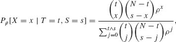
where t ![]() s = min (t, s) and ρ is the interaction parameter given by (4.7.7). The hypothesis of no interaction is equivalent to H0: ρ = 1. Notice that for ρ = 1 the p. d. f. (4.7.9) is reduced to that of the hypergeometric distribution H(N, T, S). We compare the observed value of X to the α /2– and (1−α/2)–quantiles of the hypergeometric distribution, as in the case of comparing two binomial experiments. For a generalization to 2n contingency tables, see Zelen (1972).
s = min (t, s) and ρ is the interaction parameter given by (4.7.7). The hypothesis of no interaction is equivalent to H0: ρ = 1. Notice that for ρ = 1 the p. d. f. (4.7.9) is reduced to that of the hypergeometric distribution H(N, T, S). We compare the observed value of X to the α /2– and (1−α/2)–quantiles of the hypergeometric distribution, as in the case of comparing two binomial experiments. For a generalization to 2n contingency tables, see Zelen (1972).
4.7.4 Likelihood Ratio Tests for Categorical Data
Consider a two–way layout contingency table with m1 levels of factor A and m2 levels of factor B. The sample is of size N. The likelihood function of the vector P of s = m1 × m2 cell probabilities, P(i, j), is
(4.7.10) 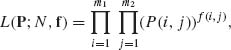
where f(i, j) are the cell frequencies. The hypothesis of no association, H0 imposes the linear restrictions on the cell probabilities
Thus, Θ0 is the parameter space restricted by (4.7.11), while Θ is the whole space of P. Thus, the likelihood ratio statistic is
(4.7.12) 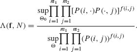
By taking the logarithm of the numerator and imposing the constraint that
we obtain by the usual methods that the values that maximize it are
(4.7.13) 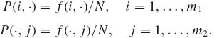
Similarly, the denominator is maximized by substituting for P(i, j) the sample estimate
(4.7.14) ![]()
We thus obtain the likelihood ratio statistic
(4.7.15) 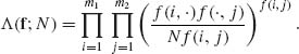
Equivalently, we can consider the test statistic −log Λ (f; N), which is
(4.7.16) 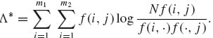
Notice that Λ* is the empirical Kullback–Leibler information number to discriminate between the actual frequency distribution f(i, j)/N and the one corresponding to the null hypothesis f(i, ·)f(·, j)/N2. This information discrimination statistic is different from the X2 statistic given in (4.7.6). In large samples, 2Λ* has the same asymptotic χ2[ν] distribution with ν = (m1−1)(m2−1). In small samples, however, it performs differently.
For further reading and extensive bibliography on the theory and methods of contingency tables analysis, see Haberman (1974), Bishop, Fienberg, and Holland (1975), Fienberg (1980), and Agresti (1990). For the analysis of contingency tables from the point of view of information theory, see Kullback (1959, Chapter 8) and Gokhale and Kullback (1978).
4.8 SEQUENTIAL TESTING OF HYPOTHESES
Testing of hypotheses may become more efficient if we can perform the sampling in a sequential manner. After each observation (group of observations) we evaluate the results obtained so far and decide whether to terminate sampling and accept (or reject) the hypothesis H0, or whether to continue sampling and observe an additional (group of) observation(s). The main problem of sequential analysis then is to determine the “best” stopping rule. After sampling terminates, the test function applied is generally of the generalized likelihood ratio type, with critical levels associated with the stopping rule, as will be described in the sequel. Early attempts to derive sequential testing procedures can be found in the literature on statistical quality control (sampling inspection schemes) of the early 1930s. The formulation of the general theory was given by Wald (1945). Wald’s book on sequential analysis (1947) is the first important monograph on the subject. The method developed by Wald is called the Wald Sequential Probability Ratio Test (SPRT). Many papers have been written on the subject since Wald’s original work. The reader is referred to the book of Ghosh (1970) for discussion of the important issues and the significant results, as well as notes on the historical development and important references. See also Siegmund (1985). We provide in Section 4.8.1 a brief exposition of the basic theory of the Wald SPRT for testing two simple hypotheses. Some remarks are given about extension for testing composite hypotheses and about more recent development in the literature. In Section 4.8.2, we discuss sequential tests that can achieve power one.
4.8.1 The Wald Sequential Probability Ratio Test
Let X1, X2, … be a sequence of i. i. d. random variables. Consider two simple hypotheses H0 and H1, according to which the p. d. f. s of these random variables are f0(x) or f1(x), respectively. Let R(Xi) = f1(Xi)/f0(Xi) i = 1, 2, … be the likelihood ratio statistics. The SPRT is specified by two boundary points A, B, −∞ < A < 0 < B < ∞ and the stopping rule, according to which sampling continues as long as the partial sums Sn = ![]() log R(Xi), n = 1, 2, …, lie between A and B. As soon as Sn ≤ A or Sn ≥ B, sampling terminates. In the first case, H0 is accepted and in the second case, H1 is accepted. The sample size N is a random variable that depends on the past observations. More precisely, the event {N ≤ n} depends on {X1, …, Xn} but is independent of {Xn+1, Xn+2, … } for all n = 1, 2, …. Such a nonnegative integer random variable is called a stopping variable. Let
log R(Xi), n = 1, 2, …, lie between A and B. As soon as Sn ≤ A or Sn ≥ B, sampling terminates. In the first case, H0 is accepted and in the second case, H1 is accepted. The sample size N is a random variable that depends on the past observations. More precisely, the event {N ≤ n} depends on {X1, …, Xn} but is independent of {Xn+1, Xn+2, … } for all n = 1, 2, …. Such a nonnegative integer random variable is called a stopping variable. Let ![]() n denote the σ–field generated by the random variables Zi = log R(Xi), i = 1, …, n. A stopping variable N defined with respect to Z1, Z2, … is an integer valued random variable N, N ≥ 1, such that the event {N ≥ n} is determined by Z1, …, Zn−1 (n ≥ 2). In this case, we say that {N ≥ n}
n denote the σ–field generated by the random variables Zi = log R(Xi), i = 1, …, n. A stopping variable N defined with respect to Z1, Z2, … is an integer valued random variable N, N ≥ 1, such that the event {N ≥ n} is determined by Z1, …, Zn−1 (n ≥ 2). In this case, we say that {N ≥ n} ![]()
![]() n−1 and I{N ≥ n} is
n−1 and I{N ≥ n} is ![]() n−1 measurable. We will show that for any pair (A, B), the stopping variable N is finite with probability one. Such a stopping variable is called regular. We will see then how to choose the boundaries (A, B) so that the error probability α and β will be under control. Finally, formulae for the expected sample size will be derived and some optimal properties will be discussed.
n−1 measurable. We will show that for any pair (A, B), the stopping variable N is finite with probability one. Such a stopping variable is called regular. We will see then how to choose the boundaries (A, B) so that the error probability α and β will be under control. Finally, formulae for the expected sample size will be derived and some optimal properties will be discussed.
In order to prove that the stopping variable N is finite with probability one, we have to prove that
Equivalently, for a fixed integer r (as large as we wish)
(4.8.2) ![]()
For θ = 0 or 1, let
(4.8.3) ![]()
and
(4.8.4) ![]()
Assume that
If D2(θ) for some θ, then (4.8.1) holds trivially at that θ.
Thus, for any value of θ, the distribution of Sn = ![]() log R(Xi) is asymptotically normal. Moreover, for each m = 1, 2, … and a fixed integer r,
log R(Xi) is asymptotically normal. Moreover, for each m = 1, 2, … and a fixed integer r,
(4.8.6) ![]()
where C = |B − A|.
The variables Sr, S2r − Sr, …, Smr − S(m−1)r are independent and identically distributed. Moreover, by the Central Limit Theorem, if r is sufficiently large,
The RHS of (4.8.7) approaches 1 as r→ ∞. Accordingly for any ρ, 0 < ρ < 1, if r is sufficiently large, then Pθ [|Sr| < c] < ρ. Finally, since Sjr − S(j−1)r is distributed like Sr for all j = 1, 2, …, r, if r is sufficiently large, then
This shows that Pθ [N > n] converges to zero at an exponential rate. This property is called the exponential boundedness of the stopping variables (Wijsman, 1971). We prove now a very important result in sequential analysis, which is not restricted only to SPRTs.
Theorem 4.8.1 (Wald Theorem) If N is a regular stopping variable with finite expectation Eθ {N}, and if X1, X2, … is a sequence of i. i. d. random variables such that Eθ {|X1| < ∞, then
(4.8.9) 
where
![]()
Proof. Without loss of generality, assume that X1, X2, … is a sequence of i. i. d. absolutely continuous random variables. Then,
where f(xn;θ) is the joint p. d. f. of Xn = (X1, …, Xn). The integral in (4.8.10) is actually an n–tuple integral. Since Eθ {|X1|} < ∞, we can interchange the order of summation and integration and obtain
(4.8.11) 
However, the event {N ≥ j} is determined by (X1, …, Xj−1) and is therefore independent of Xj, Xj+1, …. Therefore, due to the independence of the Xs,
(4.8.12) 
Finally, since N is a positive integer random variable with finite expectation,
(4.8.13) 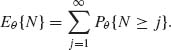 QED
QED
From assumption (4.8.5) and the result (4.8.8), both μ (θ) and Eθ {N} exist (finite). Hence, for any SPRT, Eθ {SN} = μ (θ) Eθ {N}. Let π (θ) denote the probability of accepting H0. Thus, if μ (θ)≠ 0,
(4.8.14) ![]()
An approximation to Eθ {N} can then be obtained by substituting A for Eθ {SN | SN ≤ A} and B for Eθ {SN| SN ≥ B}. This approximation neglects the excess over the boundaries by SN. One obtains
Error formulae for (4.8.15) can be found in the literature (Ghosh, 1970).
Let α and β be the error probabilities associated with the boundaries A, B and let A′ = log ![]() , B′ = log
, B′ = log ![]() . Let α′ and β′ be the error probabilities associated with the boundaries A′, B′.
. Let α′ and β′ be the error probabilities associated with the boundaries A′, B′.
Theorem 4.8.2 If 0 < α + β < 1 then
and
Proof. For each n = 1, 2, … define the sets
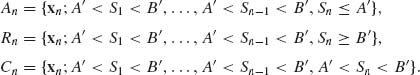
The error probability α′ satisfies the inequality
(4.8.16) 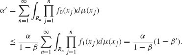
Similarly,
(4.8.17) 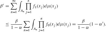
Thus,
(4.8.18) ![]()
From these inequalities we obtain the first statement of the theorem. To establish (ii) notice that if ![]() n = {x: A < Si < B, i = 1, …, n−1, Sn > B}, then
n = {x: A < Si < B, i = 1, …, n−1, Sn > B}, then
(4.8.19) 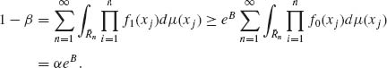
Hence, B′ = log ![]() ≥ B. The other inequality is proven similarly. QED
≥ B. The other inequality is proven similarly. QED
It is generally difficult to determine the values of A and B to obtain the specified error probabilities α and β. However, according to the theorem, if α and β are small then, by considering the boundaries A′ and B′, we obtain a procedure with error probabilities α′ and β′ close to the specified ones and total test size α′ + β′ smaller than α + β. For this reason A′ and B′ are generally used in applications. We derive now an approximation to the acceptance probability π (θ). This approximation is based on the following important identity.
Theorem 4.8.3 (Wald Fundamental Identity). Let N be a stopping variable associated with the Wald SPRT and Mθ (t) be the moment generating function (m. g. f.) of Z = log R(X). Then
(4.8.20) ![]()
for all t for which Mθ (t) exists.
Proof.
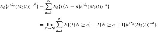
Notice that I{N ≥ n} is ![]() n−1 measurable and therefore, for n ≥ 2,
n−1 measurable and therefore, for n ≥ 2,
(4.8.22) ![]()
and Eθ {I{N ≥ 1} etS1 (Mθ (t))−1} = 1. Substituting these in (4.8.21), we obtain
![]()
Notice that E{etSm (M(t))−m} = 1 for all m = 1, 2, … and all t in the domain of convergence of Mθ (t). Thus, {etSm (Mθ (t))−m, m ≥ 1} is uniformly integrable. Finally, since ![]() P{N > m} = 0,
P{N > m} = 0,
![]() QED
QED
Choose ![]() > 0 so that,
> 0 so that,
(4.8.23) ![]()
and
![]()
Then for t > 0, Mθ (t) = Eθ {etZ} ≥ P1et![]() . Similarly, for t < 0, Mθ (t) ≥ P2e−t
. Similarly, for t < 0, Mθ (t) ≥ P2e−t![]() . This proves that
. This proves that ![]() Mθ (t) = ∞. Moreover, for all t for which M(t) exists,
Mθ (t) = ∞. Moreover, for all t for which M(t) exists,
(4.8.24) 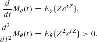
Thus, we deduce that the m. g. f. Mθ (t) is a strictly convex function of t. The expectation μ (θ) is M′θ (0). Hence, if μ (θ) > 0 then Mθ (t) attains its unique minimum at a negative value t* and Mθ (t*) < 1. Furthermore, there exists a value t0, −∞ < t0 < t* < 0, at which Mθ (t0) = 1. Similarly, if μ (θ) < 0, there exist positive values t* and t0, 0 < t* < t0 < ∞, such that Mθ (t*) < 1 and Mθ (t0) = 1. In both cases t* and t0 are unique.
The fundamental identity can be applied to obtain an approximation for the acceptance probability π (θ) of the SPRT with boundaries A′ and B′. According to the fundamental identity
where t0(θ) ≠ 0 is the point at which Mθ (t) = 1. The approximation for π (θ) is obtained by substituting in (4.8.25)
![]()
and
![]()
This approximation yields the formula
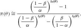
for all θ such that μ (θ) ≠ 0. If θ0 is such that μ (θ0) = 0, then
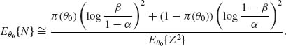
The approximation for Eθ {N} given by (4.8.15) is inapplicable at θ0. However, at θ0, Wald’s Theorem yields the result
(4.8.28) ![]()
From this, we obtain for θ0
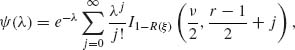
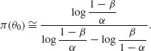
In Example 4.17, we have illustrated the use of the Wald SPRT for testing two composite hypotheses when the interval Θ0 corresponding to H0 is separated from the interval Θ1 of H1. We obtained a test procedure with very desirable properties by constructing the SPRT for two simple hypotheses, since the family ![]() of distribution functions under consideration is MLR. For such families we obtain a monotone π (θ) function, with acceptance probability greater than 1−α for all θ < θ0 and π (θ) < β for all θ > θ1 (Ghosh, 1970, pp. 100–103). The function π (θ) is called the operating characteristic function O. C. of the SPRT. The expected sample size function Eθ {N} increases to a maximum between θ0 and θ1 and then decreases to zero again. At θ = θ0 and at θ = θ1 the function Eθ {N} assumes the smallest values corresponding to all possible test procedures with error probabilities not exceeding α and β. This is the optimality property of the Wald SPRT. We state this property more precisely in the following theorem.
of distribution functions under consideration is MLR. For such families we obtain a monotone π (θ) function, with acceptance probability greater than 1−α for all θ < θ0 and π (θ) < β for all θ > θ1 (Ghosh, 1970, pp. 100–103). The function π (θ) is called the operating characteristic function O. C. of the SPRT. The expected sample size function Eθ {N} increases to a maximum between θ0 and θ1 and then decreases to zero again. At θ = θ0 and at θ = θ1 the function Eθ {N} assumes the smallest values corresponding to all possible test procedures with error probabilities not exceeding α and β. This is the optimality property of the Wald SPRT. We state this property more precisely in the following theorem.
Theorem 4.8.4 (Wald and Wolfowitz) Consider any SPRT for testing the two simple hypotheses H0: θ = θ0 against H1: θ = θ1 with boundary points (A, B) and error probabilities α and β. Let Eθi{N}, i = 0, 1 be the expected sample size. If s is any sampling procedure for testing H0 against H1 with error probabilities α (s) and β (s) and finite expected sample size Eθi{N(s)} (i = 0, 1), then α (s) ≤ α and β (s) ≤ β imply that Eθi{N} ≤ Eθi{N(s)}, for i = 0, 1.
For the proof of this important theorem, see Ghosh (1970, pp. 93–98), Siegmund (1985, p. 19). See also Section 8.2.3.
Although the Wald SPRT is optimal at θ0 and at θ1 in the above sense, if the actual θ is between θ0 and θ1, even in the MLR case, the expected sample size may be quite large. Several papers were written on this subject and more general sequential procedures were investigated, in order to obtain procedures with error probabilities not exceeding α and β at θ0 and θ1 and expected sample size at θ0 < θ < θ1 smaller than that of the SPRT. Kiefer and Weiss (1957) studied the problem of determining a sequential test that, subject to the above constraint on the error probabilities, minimizes the maximal expected sample size. They have shown that such a test is a generalized version of an SPRT. The same problem was studied recently by Lai (1973) for normally distributed random variables using the theory of optimal stopping rules. Lai developed a method of determining the boundaries {(An, Bn), n ≥ 1} of the sequential test that minimizes the maximal expected sample size. The theory required for discussing this method is beyond the scope of this chapter. We remark in conclusion that many of the results of this section can be obtained in a more elegant fashion by using the general theory of optimal stopping rules. The reader is referred in particular to the book of Chow, Robbins, and Siegmund (1971). For a comparison of the asymptotic relative efficiency of sequential and nonsequential tests of composite hypotheses, see Berk (1973, 1975). A comparison of the asymptotic properties of various sequential tests (on the means of normal distributions), which combines both the type I error probability and the expected sample size, has been provided by Berk (1976).
PART II: EXAMPLES
Example 4.1. A new drug is being considered for adoption at a medical center. It is desirable that the probability of success in curing the disease under consideration will be at least θ0 = .75. A random sample of n = 30 patients is subjected to a treatment with the new drug. We assume that all the patients in the sample respond to the treatment independently of each other and have the same probability to be cured, θ. That is, we adopt a Binomial model B(30, θ) for the number of successes in the sample. The value θ0 = .75 is the boundary between undesirable and desirable cure probabilities. We wish to test the hypothesis that θ ≥.75.
If the number of successes is large the data support the hypothesis of large θ value. The question is, how small could be the observed value of X, before we should reject the hypothesis that θ ≥.75. If X = 18 and we reject the hypothesis then α (18) = B(18; 30,.75) = .05066. This level of significance is generally considered sufficiently small and we reject the hypothesis if X ≤ 18. ![]()
Example 4.2. Let X1, X2, …, Xn be i. i. d. random variables having a common rectangular distribution R(0, θ), 0 < θ < ∞. We wish to test the hypothesis H0: θ ≤ θ0 against the alternative H1: θ > θ0. An m. s. s. is the sample maximum X(n). Hence, we construct a test function of size α, for some given α in (0, 1), which depends on X(n). Obviously, if X(n) ≥ θ0 we should reject the null hypothesis. Thus, it is reasonable to construct a test function ![]() (X(n)) that rejects H0 whenever X(n) ≥ Cα. Cα depends on α and θ0, i. e.,
(X(n)) that rejects H0 whenever X(n) ≥ Cα. Cα depends on α and θ0, i. e.,
![]()
Cα is determined so that the size of the test will be α. At θ = θ0,
![]()
Hence, we set Cα = θ0(1−α)1/n. The power function, for all θ > θ0, is
![]()
We see that ![]() (θ) is greater than α for all θ > θ0. On the other hand, for θ ≤ θ0, the probability of rejection is
(θ) is greater than α for all θ > θ0. On the other hand, for θ ≤ θ0, the probability of rejection is
![]()
Accordingly, the maximal probability of rejection, when H0 is true, is α and if θ < θ0, the probability of rejection is smaller than α. Obviously, if θ ≤ θ0(1−α)1/n, then the probability of rejection is zero.. ![]()
Example 4.3. Let X1, …, Xn be i. i. d. random variables having a normal distribution N(μ, σ2). According to the null hypothesis H0: μ = μ1, σ = σ1. According to the alternative hypothesis H1: μ = μ2, σ = σ2; σ2 > σ1. The likelihood ratio is
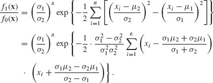
We notice that the distribution function of f1(X)/f0(X) is continuous and therefore γα = 0. According to the Neyman–Pearson Lemma, a most powerful test of size α is obtained by rejecting H0 whenever f1(X)/f0(X) is greater than some positive constant kα. But, since σ2 > σ1, this is equivalent to the test function that rejects H0 whenever
![]()
where Cα is an appropriate constant. Simple algebraic manipulations yield that H0 should be rejected whenever
![]()
where
![]()
We find ![]() in the following manner. According to H0,
in the following manner. According to H0,
![]()
with δ = σ![]() (μ2 − μ1)/(
(μ2 − μ1)/(![]() − σ
− σ![]() ). It follows that
). It follows that ![]() (Xi − ω)2 ~ σ
(Xi − ω)2 ~ σ![]() χ2[n;nδ2/2σ
χ2[n;nδ2/2σ![]() ] and thus,
] and thus,
![]()
where ![]() [ν ;λ] is the (1−α)th quantile of the noncentral χ2. We notice that if μ1 = μ2 but σ1 ≠ σ2, the two hypotheses reduce to the hypotheses
[ν ;λ] is the (1−α)th quantile of the noncentral χ2. We notice that if μ1 = μ2 but σ1 ≠ σ2, the two hypotheses reduce to the hypotheses ![]() : μ1 = μ, σ2 = σ
: μ1 = μ, σ2 = σ![]() versus
versus ![]() : μ2 = μ, σ2 ≠ σ1. In this case, δ = 0 and
: μ2 = μ, σ2 ≠ σ1. In this case, δ = 0 and ![]() . If σ1 = σ2 but μ2 > μ1 (or μ2 < μ1), the test reduces to the t–test of Example 4.9..
. If σ1 = σ2 but μ2 > μ1 (or μ2 < μ1), the test reduces to the t–test of Example 4.9.. ![]()
Example 4.4. In this example, we present a case of testing the shape parameter of a Weibull distribution. This case is important in reliability life testing. We show that even if the problem is phrased in terms of two simple hypotheses, it is not a simple matter to determine the most powerful test function. This difficulty is due to the fact that if the shape parameter is unknown, the minimal sufficient statistic is the order statistic. Let X1, …, Xn be i. i. d. random variables having a common Weibull distribution G1/ν(1, 1). We wish to test the null hypothesis H0: ν = 1 against the simple alternative H1: ν = 1 + δ; δ is a specified positive number. Notice that under H0, Xi ~ E(1), i. e., exponentially distributed with mean 1. According to the Neyman–Pearson Lemma, the most powerful test of size α rejects H0 whenever
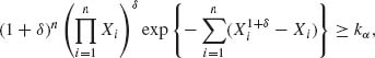
where kα is determined so that if H0 is correct, then the probability is exactly α. Equivalently, we have to determine a constant cα so that, under H0, the probability of
![]()
is exactly α. Let Wi(δ) = log Xi − ![]() and Sn(δ) =
and Sn(δ) = ![]() Wi(δ). The problem is to determine the distribution of Sn(δ) under H0. If n is large, we can approximate the distribution of Sn(δ) by a normal distribution. The expected value of W(δ) is
Wi(δ). The problem is to determine the distribution of Sn(δ) under H0. If n is large, we can approximate the distribution of Sn(δ) by a normal distribution. The expected value of W(δ) is
![]()
where Γ′(1) is the derivative of Γ (x) at x = 1. The second moment of W(δ) is
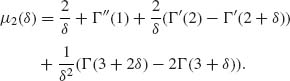
Thus, according to the Central Limit Theorem, if n is sufficiently large, then
![]()
Accordingly, for large values of n, the critical level Cα is approximately
![]()
For small values of n, we can determine Cα approximately by simulating many replicas of Sn(δ) values when X1, …, Xn are E(1) and determining the (1−α)th quantile point of the empirical distribution of Sn(δ).. ![]()
Example 4.5. Consider an experiment in which n Bernoulli trials are performed. Let K denote the number of successes among these trials and let θ denote the probability of success. Suppose that we wish to test the hypothesis
![]()
at level of significance α. θ0 and α are specified numbers. The UMP (randomized) test function is
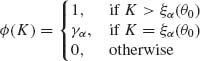
where ξα (θ0) is the (1−α)–quantile of the binomial distribution B(n, θ0), i. e.,
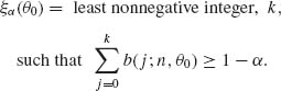
Furthermore,
![]()
Accordingly, if the number of successes K is larger than the (1−α)–quantile of B(n, θ0), we reject H0. If K equals ξα (θ0), the null hypothesis H0 is rejected only with probability γα. That is, a random number R having a R(0, 1) distribution is picked from a table of random numbers. If K = ξα (θ0) and R ≤ γα, H0 is rejected; if K = ξα (θ0) and R > γα, then H0 is accepted. If K < ξα (θ0), H0 is accepted. It is easy to verify that if θ = θ0 then the probability of rejecting H0 is exactly α. If θ < θ0 this probability is smaller than α and, on the other hand, if θ > θ0 the probability of rejection is greater than α. The test of this one–sided hypothesis H0 can be easily performed with the aid of tables of the cumulative binomial distributions. The exact power of the test can be determined according to the formula
![]()
where θ > θ0. If the hypotheses are one–sided but to the other direction, i. e., H0: θ ≥ θ0 against H1: θ < θ0, the UMP test is similar.. ![]()
Example 4.6. Consider the family ![]() of Poisson distributions P(θ), 0 < θ < ∞. The p. d. f. s are
of Poisson distributions P(θ), 0 < θ < ∞. The p. d. f. s are
![]()
Thus, if we make the reparametrization ω = log θ, then
![]()
This is a one–parameter exponential type family. The hypotheses H0: θ = θ0 against H1: θ ≠ θ0 (0 < θ0 < ∞) are equivalent to the hypotheses H0: ω = ω0 against H1: ω ≠ ω0 where ω0 = log θ0. The two–sided test ![]() 0(X) of size α is obtained by (4.4.1), where the constants are determined according to the conditions (4.4.2) and (4.4.6). Since
0(X) of size α is obtained by (4.4.1), where the constants are determined according to the conditions (4.4.2) and (4.4.6). Since ![]() is Poisson, Eθ0{X} = θ0. Moreover, the p. d. f. of P(θ) satisfies the relation
is Poisson, Eθ0{X} = θ0. Moreover, the p. d. f. of P(θ) satisfies the relation
![]()
We thus obtain the equations, for x1 = ![]() and x2 =
and x2 = ![]() , γ1 and γ2:
, γ1 and γ2:
![]()
Here P(j;θ) is the Poisson c. d. f. The function is zero whenever the argument j is negative. The determination of x1, γ1, x2, γ2 can be done numerically. We can start with the initial solution x1, γ1 and x2, γ2 corresponding to the “equal–tail” test. These initial values are determined from the equations
![]()
This initial solution can then be modified so that both equations (i) and (ii) will be satisfied simultaneously.. ![]()
Example 4.7. Suppose that X ~ N(θ, 1). The null hypothesis is H0: θ = 0. The alternative is H1: θ ≠ 0. Thus, x1 and x2 should satisfy simultaneously the two equations
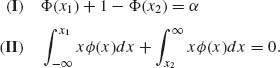
Notice that x![]() (x) = −
(x) = −![]() ′(x). Accordingly, equation (II) can be written as
′(x). Accordingly, equation (II) can be written as
![]()
If we set x1 = z1−α /2 and x2 = −x1 where zγ = Φ−1(γ) then, due to the symmetry of the N(0, 1) distribution around θ = 0, we obtain that these x1 and x2 satisfy simultaneously the two equations. The “equal–tail” solution is the desired solution in this case.. ![]()
Example 4.8. A. Testing the Significance of the Mean in Normal Samples
The problem studied is that of testing hypotheses about the mean of a normal distribution. More specifically, we have a sample X1, …, Xn of i. i. d. random variables from a normal distribution N(μ, σ2). We test the hypothesis
![]()
against
![]()
The m. s. s. is (![]() n, Qn), where
n, Qn), where ![]() n =
n = ![]()
![]() Xi and Qn =
Xi and Qn = ![]() (Xi −
(Xi − ![]() n)2. Consider the t–statistic t =
n)2. Consider the t–statistic t = ![]() (
(![]() n − μ)/Sn, where
n − μ)/Sn, where ![]() = Qn/(n−1). The t–test of H0 against H1 is given by
= Qn/(n−1). The t–test of H0 against H1 is given by
![]()
t1-α /2[n−1] is the (1−α /2)–quantile of the t–distribution with n−1 degrees of freedom. It is easy to verify that this t–test has the size α. Its power function can be determined in the following manner. If μ ≠ μ0 then
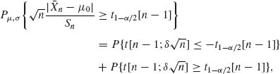
where δ = (μ − μ0)/σ. According to (2.12.22), this power function can be computed according to the formula
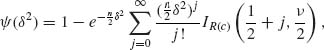
where ν = n−1, c = t1−α /2 [n−1] and R(c) = c2/(ν + c2). We notice that the power function depends on δ2 and is therefore symmetric around δ0 = 0. We prove now that the t–test is unbiased. Rewrite the power function as a function of ![]() and a mixture of Poisson P(λ) with
and a mixture of Poisson P(λ) with ![]() , where J ~ P(λ) and R(c) = c2/(ν + c2). The family P(λ) is MLR in J. Moreover,
, where J ~ P(λ) and R(c) = c2/(ν + c2). The family P(λ) is MLR in J. Moreover, ![]() is a decreasing function of j. Hence, by Karlin’s Lemma,
is a decreasing function of j. Hence, by Karlin’s Lemma, ![]() is an increasing function of λ. Moreover,
is an increasing function of λ. Moreover, ![]() (0) = α. This proves that the test is unbiased.
(0) = α. This proves that the test is unbiased.
B. Testing the Significance of the Sample Correlation
(X1, Y1), …, (Xn, Yn) are i. i. d. random vectors having a bivariate normal distribution. Let r be the sample coefficient of correlation (formula 2.13.1). Consider the problem of testing the hypothesis H0: ρ ≤ 0, (μ1, μ2, σ1, σ2) arbitrary; against H1: ρ > 0, (μ1, μ2, σ1, σ2) arbitrary. Here we have four nuisance parameters. As shown in Section 2.15, the distribution of r is independent of the nuisance parameters (μ1, μ2, σ1, σ2) and when ρ = 0 (on the boundary between Θ0 and Θ1), it is independent of all the parameters. Moreover, according to (2.13.11), the following test is boundary α–similar.
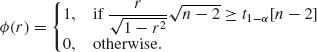
The power function depends only on the parameter ρ and is given by
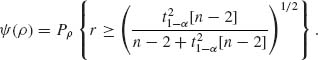
According to (2.13.12), this is equal to
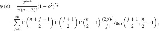
where R(t) = (n − 2)/(n−2 + ![]() [n − 2]. To show that this power function is a monotone nondecreasing function of ρ, one can prove that the family of densities of r under ρ (2.13.12) is an MLR with respect to r. Therefore, according to Karlin’s Lemma, Eρ {
[n − 2]. To show that this power function is a monotone nondecreasing function of ρ, one can prove that the family of densities of r under ρ (2.13.12) is an MLR with respect to r. Therefore, according to Karlin’s Lemma, Eρ {![]() (r)} is a nondecreasing function of ρ. Thus, the test function
(r)} is a nondecreasing function of ρ. Thus, the test function ![]() (r) is not only boundary α–similar but also unbiased..
(r) is not only boundary α–similar but also unbiased.. ![]()
Example 4.9. Let X and Y be independent r. v. s having Poisson distributions with means λ1 and λ2, respectively. We wish to test the hypotheses H0: λ1 = λ2 against H1: λ1 ≠ λ2. Let T = X + Y. The conditional distribution of X given T is the binomial B(T, p) where p = λ1/(λ1 + λ2). The marginal distribution of T is P(ν) where ν = λ1 + λ2. We can therefore write the joint p. d. f. of X and T in the form
![]()
where θ = log (λ1/λ2) and τ = log λ2. Thus, the hypotheses under consideration are equivalent to H0: θ = 0, τ arbitrary; against H1: θ ≠ 0, τ arbitrary.
Accordingly, we consider the two–sided test functions
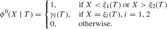
This test is uniformly most powerful unbiased of size α if the functions ξi(T) and γi(T), i = 1, 2, are determined according to the conditional distribution of X given T, under H0. As mentioned earlier, this conditional distribution is the binomial B(T, ![]() ). This is a symmetric distribution around X0 = T/2. In other words, b(i; T,
). This is a symmetric distribution around X0 = T/2. In other words, b(i; T, ![]() ) = b(T−i; T,
) = b(T−i; T, ![]() ), for all i = 0, …, T. Conditions (4.5.9) are equivalent to
), for all i = 0, …, T. Conditions (4.5.9) are equivalent to
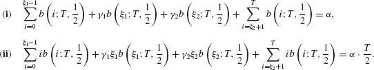
It is easy to verify that, due to the symmetry of the Binomial B(T, ![]() ), the functions that satisfy (i) and (ii) are
), the functions that satisfy (i) and (ii) are
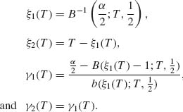
Here ![]() is the
is the ![]() –quantile of B(T,
–quantile of B(T, ![]() ) and B(j; T,
) and B(j; T, ![]() ) is the c. d. f. of B(T,
) is the c. d. f. of B(T, ![]() ) at X = j..
) at X = j.. ![]()
Example 4.10. In a clinical trial we test the effect of a certain treatment, in comparison to some standard treatment, at two different stations. The null hypothesis is that the effect of the two treatments relative to the control is the same at the two stations. For this objective, a balanced experiment is conducted in which 2n patients are tested at each station, n patients with the new treatment and n with the standard one. The observed random variables, Xij (i = 1, 2; j = 1, 2) are the number of successes in each sample of n. There are four independent binomial random variables. Let θij (i, j = 1, 2) denote the probability of success. i = 1, 2 denotes the station index and j = 1, 2 denotes the treatment index (j = 1 for the standard treatment and j = 2 for the new treatment). Thus Xij ~ B(n, θij). Let Ti = Xi1 + Xi2 (i = 1, 2) and
![]()
Let Yi = Xi1 (i = 1, 2). The conditional p. d. f. of Yi given Ti is the confluent hypergeometric function
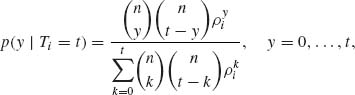
where generally ![]() if b > a. We notice that when ρi = 1 (i. e., θi1 = θi2), then the p. d. f. is the hypergeometric p. d. f. h(y| 2n, n, t) as given by (2.3.6). Thus, since Y1 and Y2 are independent, the joint conditional p. d. f. of (Y1, Y2) given T1 = t and T2 = v under (ρ1, ρ2) is
if b > a. We notice that when ρi = 1 (i. e., θi1 = θi2), then the p. d. f. is the hypergeometric p. d. f. h(y| 2n, n, t) as given by (2.3.6). Thus, since Y1 and Y2 are independent, the joint conditional p. d. f. of (Y1, Y2) given T1 = t and T2 = v under (ρ1, ρ2) is
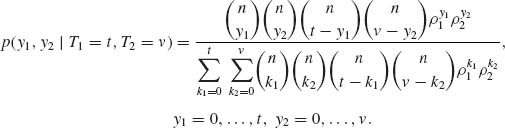
We consider the problem of testing the hypotheses:
![]()
Our hypothesis H0 means that there is no interaction between the effect of the treatment and that of the station. We notice now that under H0, S = Y1 + Y2 is a sufficient statistic for the family of joint conditional distributions given T1 and T2. Furthermore, the conditional p. d. f. of Y1 given T1, T2, and S is
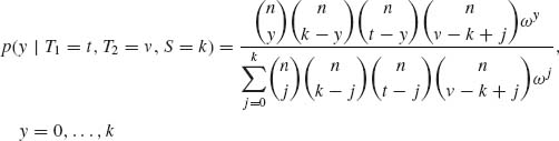
where ω = ρ1/ρ2. The family of all the conditional distributions of Y1 given (T1, T2, S) is an MLR family w. r. t. Y1. The hypotheses H0: ρ1 = ρ2 against H1: ρ1 ≠ ρ2 are equivalent to the hypotheses H0: ω = 1 against H1: ω ≠ 1. Accordingly, the conditional test function
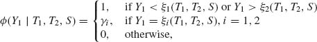
is uniformly most powerful unbiased of size α, if the functions ξi(T1, T2, S) and γi(T1, T2, S) are determined to satisfy conditions (i) and (ii) of (4.5.9) simultaneously. To prove it, we have to show that the family of conditional joint distributions of S given (T1, T2) is complete and that the power function of every test function is continuous in (θ11, θ12, θ21, θ22). This is left to the reader as an exercise. For the computation of the power function and further investigation, see Zacks and Solomon (1976).. ![]()
Example 4.11. A. In this example we show that the t–test, which was derived in Example 4.9, is uniformly most powerful unbiased. An m. s. s. for the family of normal distributions ![]() = {N(μ, σ2); −∞ < μ < ∞, 0 < σ < ∞ } is (Σ Xi, Σ
= {N(μ, σ2); −∞ < μ < ∞, 0 < σ < ∞ } is (Σ Xi, Σ ![]() ). Let U =
). Let U = ![]() Σ Xi and T = Σ
Σ Xi and T = Σ ![]() . We notice that T is an m. s. s. for
. We notice that T is an m. s. s. for ![]() * (the family restricted to the boundary, μ = 0). Consider the statistic
* (the family restricted to the boundary, μ = 0). Consider the statistic ![]() . We notice that if μ = 0, then W ~ t[n−1] independently of σ2. On the other hand, T~ σ2χ2[n] when μ = 0. Therefore, according to Basu’s Theorem, W and T are independent for each θ
. We notice that if μ = 0, then W ~ t[n−1] independently of σ2. On the other hand, T~ σ2χ2[n] when μ = 0. Therefore, according to Basu’s Theorem, W and T are independent for each θ ![]() Θ* (the boundary) since the family
Θ* (the boundary) since the family ![]() T is complete. Furthermore, W is an increasing function of U for each T. Hence, the t–test is uniformly most powerful unbiased.
T is complete. Furthermore, W is an increasing function of U for each T. Hence, the t–test is uniformly most powerful unbiased.
B. Consider part (B) of Example 4.9. The m. s. s. is (Σ Xi, Σ ![]() , Σ Yi, Σ
, Σ Yi, Σ![]() , Σ Xi Yi). If we denote by
, Σ Xi Yi). If we denote by ![]() * the family of all bivariate normal distributions with ρ = 0 (corresponding to the boundary), then T = (ΣXi, Σ
* the family of all bivariate normal distributions with ρ = 0 (corresponding to the boundary), then T = (ΣXi, Σ ![]() , Σ Yi, Σ
, Σ Yi, Σ ![]() ) is an m. s. s. for
) is an m. s. s. for ![]() *. Let U = Σ XiYi. The sample correlation coefficient r is given by
*. Let U = Σ XiYi. The sample correlation coefficient r is given by
![]()
This function is increasing in U for each T. We notice that the distribution of r is independent of ν = (μ1, μ2, σ1, σ2). Therefore, r is independent of T for each ν whenever ρ = 0. The test function ![]() (r) of Example 4.9 is uniformly most powerful unbiased to test H0: ρ ≤ 0, ν arbitrary, against H1: ρ > 0, ν arbitrary.
(r) of Example 4.9 is uniformly most powerful unbiased to test H0: ρ ≤ 0, ν arbitrary, against H1: ρ > 0, ν arbitrary. ![]()
Example 4.12. Consider again the components of variance Model II of Analysis of Variance, which is discussed in Example 3.9. Here, we have a three–parameter family of normal distributions with parameters μ, σ2, and τ 2. We set ρ = τ2/σ2.
A. For testing the hypotheses
![]()
against
![]()
the t–test
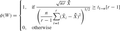
is a uniformly most powerful unbiased one. Indeed, if we set U = T3(X) = ![]() , T = (T1(X), T2(X)), then
, T = (T1(X), T2(X)), then 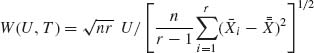 is distributed when μ = 0, as t[r−1] for all (σ2, ρ). The exponential family is complete. Hence, W(U, T) and T are independent for each (σ2, ρ) when μ = 0. Furthermore, W(U, T) is an increasing function of U for each T.
B. For testing the hypotheses
![]()
against
![]()
the test function
![]()
is uniformly most powerful unbiased. Here
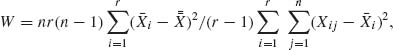
and F1−α [r−1, r(n−1)] is the (1−α)–quantile of the central F–distribution with (r−1) and r(n−1) degrees of freedom. ![]()
Example 4.13. Let X ~ N(θ, 1). We consider the two simple hypotheses H0: θ = 0 versus H1: θ = 1. The statistic Λ (X) is
![]()
Obviously, Λ (X) = 1 if and only if X ≤ ![]() . It follows that, under θ = 0, P0[Λ (X) = 1] = Φ (
. It follows that, under θ = 0, P0[Λ (X) = 1] = Φ (![]() ) = .691. Therefore, in this example, the generalized likelihood ratio test can be performed only for α ≤ 1 −.691 = .309 or for α = 1. This is a restriction on the generalized likelihood ratio test. However, generally we are interested in small values of α, for which the test exists.
) = .691. Therefore, in this example, the generalized likelihood ratio test can be performed only for α ≤ 1 −.691 = .309 or for α = 1. This is a restriction on the generalized likelihood ratio test. However, generally we are interested in small values of α, for which the test exists. ![]()
Example 4.14. Let X1, …, Xn be i. i. d. random variables having a common Laplace distribution with p. d. f.
![]()
where the parameter space is Θ = {−∞ < θ < ∞ }. We wish to test
![]()
against
![]()
The sample statistic ![]() , which minimizes
, which minimizes ![]() |xi − θ|, is the sample median
|xi − θ|, is the sample median
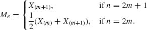
Thus, the generalized likelihood statistic is
λ (Xn) is sufficiently small if
![]()
is sufficiently large. To obtain a size α test, we need the (1 − α)–quantile of the sampling distribution of T(Xn) under θ = 0. M = 1000 simulation runs, using S–PLUS, gave the following estimates of the 95th quantile of T(Xn).
Notice that −2 log Λ (Xn) = 2· T(Xn) and that ![]() [1] = 3.8415. Also 2
[1] = 3.8415. Also 2 ![]() .95, n
.95, n ![]()
![]() [1].
[1].
![]() .
. ![]()
Example 4.15. Fleiss (1973, p. 131) gave the following 2 × 2 table of G–6–PD deficiency (A) and type of schizophrenia (B) among N = 177 patients.
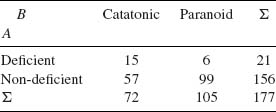
We test whether the association between the two variables is significant. The X2 statistic for this table is equal to 9.34. This is greater than ![]() [1] = 3.84 and therefore significant at the α = .05 level. To perform the conditional test we compute the hypergeometric distribution H(N, T, S) with N = 177, T = 21, and S = 72. In Table 4.3, we present the p. d. f. h(x; N, T, S) and the c. d. f. H(x; N, T, S) of this distribution.
[1] = 3.84 and therefore significant at the α = .05 level. To perform the conditional test we compute the hypergeometric distribution H(N, T, S) with N = 177, T = 21, and S = 72. In Table 4.3, we present the p. d. f. h(x; N, T, S) and the c. d. f. H(x; N, T, S) of this distribution.
According to this conditional distribution, with α = .05, we reject H0 whenever X ≤ 4 or X ≥ 14. If X = 5 we reject H0 only with probability γ1 = .006. If X = 13 we reject H0 with probability γ2 = .699. In this example, X = 15 and therefore we conclude that the association is significant.. ![]()
Table 4.3 The Hypergeometric Distribution H(177, 21, 72)
| x | h(x; N, T, S) | H(x; N, T, S) |
| 0 | 0.000007 | 0.000007 |
| 1 | 0.000124 | 0.000131 |
| 2 | 0.001022 | 0.001153 |
| 3 | 0.005208 | 0.006361 |
| 4 | 0.018376 | 0.024736 |
| 5 | 0.047735 | 0.072471 |
| 6 | 0.094763 | 0.167234 |
| 7 | 0.147277 | 0.314511 |
| 8 | 0.182095 | 0.496607 |
| 9 | 0.181006 | 0.677614 |
| 10 | 0.145576 | 0.823190 |
| 11 | 0.095008 | 0.918198 |
| 12 | 0.050308 | 0.968506 |
| 13 | 0.021543 | 0.990049 |
Example 4.16. Let X1, X2, … be a sequence of i. i. d. random variables having a common normal distribution N(θ, 1), −∞ < θ < ∞. Suppose that for testing the hypothesis H0: θ ≤ 0 against H1: θ ≥ 1, we construct the Wald SPRT of the two simply hypotheses ![]() : θ = 0 against
: θ = 0 against ![]() : θ = 1 with boundaries A′ and B′ corresponding to α = .05 and β = .05.
: θ = 1 with boundaries A′ and B′ corresponding to α = .05 and β = .05.
Notice that
![]()
Accordingly,
![]()
The m. g. f. of Z at θ is
![]()
Thus, t0(θ) = 1 − 2θ, and from (4.8.26)–(4.8.27), the acceptance probabilities are
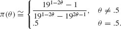
In the following table we present some of the π(θ) and Eθ{N} values, determined according to the approximations (4.8.15) and (4.8.26).
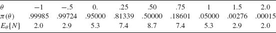
The number of observations required in a fixed sample design for testing ![]() : θ = 0 against
: θ = 0 against ![]() : θ = 1 with α = β = .05 is n = 16. According to the above table, the expected sample size in a SPRT when θ = 0 or θ = 1 is only one third of that required in a fixed sample testing..
: θ = 1 with α = β = .05 is n = 16. According to the above table, the expected sample size in a SPRT when θ = 0 or θ = 1 is only one third of that required in a fixed sample testing.. ![]()