
CHAPTER 8
Bayesian Analysis in Testing and Estimation
PART I: THEORY
This chapter is devoted to some topics of estimation and testing hypotheses from the point of view of statistical decision theory. The decision theoretic approach provides a general framework for both estimation of parameters and testing hypotheses. The objective is to study classes of procedures in terms of certain associated risk functions and determine the existence of optimal procedures. The results that we have presented in the previous chapters on minimum mean–squared–error (MSE) estimators and on most powerful tests can be considered as part of the general statistical decision theory. We have seen that uniformly minimum MSE estimators and uniformly most powerful tests exist only in special cases. One could overcome this difficulty by considering procedures that yield minimum average risk, where the risk is defined as the expected loss due to erroneous decision, according to the particular distribution Fθ. The MSE in estimation and the error probabilities in testing are special risk functions. The risk functions depend on the parameters θ of the parent distribution. The average risk can be defined as an expected risk according to some probability distribution on the parameter space. Statistical inference that considers the parameter(s) as random variables is called a Bayesian inference. The expected risk with respect to the distribution of θ is called in Bayesian theory the prior risk, and the probability measure on the parameter space is called a prior distribution. The estimators or test functions that minimize the prior risk, with respect to some prior distribution, are called Bayes procedures for the specified prior distribution. Bayes procedures have certain desirable properties. This chapter is devoted, therefore, to the study of the structure of optimal decision rules in the framework of Bayesian theory. We start Section 8.1 with a general discussion of the basic Bayesian tools and information functions. We outline the decision theory and provide an example of an optimal statistical decision procedure. In Section 8.2, we discuss testing of hypotheses from the Bayesian point of view, and in Section 8.3, we present Bayes credibility intervals. The Bayesian theory of point estimation is discussed in Section 8.4. Section 8.5 discusses analytical and numerical techniques for evaluating posterior distributions on complex cases. Section 8.6 is devoted to empirical Bayes procedures.
8.1 THE BAYESIAN FRAMEWORK
8.1.1 Prior, Posterior, and Predictive Distributions
In the previous chapters, we discussed problems of statistical inference, testing hypotheses, and estimation, considering the parameters of the statistical models as fixed unknown constants. This is the so–called classical approach to the problems of statistical inference. In the Bayesian approach, the unknown parameters are considered as values determined at random according to some specified distribution, called the prior distribution. This prior distribution can be conceived as a normalized nonnegative weight function that the statistician assigns to the various possible parameter values. It can express his degree of belief in the various parameter values or the amount of prior information available on the parameters. For the philosophical foundations of the Bayesian theory, see the books of DeFinneti (1974), Barnett (1973), Hacking (1965), Savage (1962), and Schervish (1995). We discuss here only the basic mathematical structure.
Let ![]() = {F(x; θ); θ
= {F(x; θ); θ ![]() Θ} be a family of distribution functions specified by the statistical model. The parameters θ of the elements of
Θ} be a family of distribution functions specified by the statistical model. The parameters θ of the elements of ![]() are real or vector valued parameters. The parameter space Θ is specified by the model. Let
are real or vector valued parameters. The parameter space Θ is specified by the model. Let ![]() be a family of distribution functions defined on the parameter space Θ. The statistician chooses an element H(θ) of
be a family of distribution functions defined on the parameter space Θ. The statistician chooses an element H(θ) of ![]() and assigns it the role of a prior distribution. The actual parameter value θ0 of the distribution of the observable random variable X is considered to be a realization of a random variable having the distribution H(θ). After observing the value of X the statistician adjusts his prior information on the value of the parameter θ by converting H(θ) to the posterior distribution H(θ | X). This is done by Bayes Theorem according to which if h(θ) is the prior probability density function (p.d.f.) of θ and f(x; θ) the p.d.f. of X under θ, then the posterior p.d.f. of θ is
and assigns it the role of a prior distribution. The actual parameter value θ0 of the distribution of the observable random variable X is considered to be a realization of a random variable having the distribution H(θ). After observing the value of X the statistician adjusts his prior information on the value of the parameter θ by converting H(θ) to the posterior distribution H(θ | X). This is done by Bayes Theorem according to which if h(θ) is the prior probability density function (p.d.f.) of θ and f(x; θ) the p.d.f. of X under θ, then the posterior p.d.f. of θ is
(8.1.1) ![]()
If we are given a sample of n observations or random variables X1, X2, …, Xn, whose distributions belong to a family ![]() , the question is whether these random variables are independent identically distributed (i.i.d.) given θ, or whether θ might be randomly chosen from H(θ) for each observation.
, the question is whether these random variables are independent identically distributed (i.i.d.) given θ, or whether θ might be randomly chosen from H(θ) for each observation.
At the beginning, we study the case that X1, …, Xn are conditionally i.i.d., given θ. This is the classical Bayesian model. In Section 8.6, we study the so–called empirical Bayes model, in which θ is randomly chosen from H(θ) for each observation. In the classical model, if the family ![]() admits a sufficient statistic T(X), then for any prior distribution H(θ), the posterior distribution is a function of T(X), and can be determined from the distribution of T(X) under θ. Indeed, by the Neyman–Fisher Factorization Theorem, if T(X) is sufficient for
admits a sufficient statistic T(X), then for any prior distribution H(θ), the posterior distribution is a function of T(X), and can be determined from the distribution of T(X) under θ. Indeed, by the Neyman–Fisher Factorization Theorem, if T(X) is sufficient for ![]() then f(x; θ) = k(x)g(T(x); θ). Hence,
then f(x; θ) = k(x)g(T(x); θ). Hence,
(8.1.2) ![]()
Thus, the posterior p.d.f. is a function of T(X). Moreover, the p.d.f. of T(X) is g* (t; θ) = k* (t)g(t; θ), where k* (t) is independent of θ. It follows that the conditional p.d.f. of θ given {T(X) = t} coincides with h(θ | x) on the sets {x; T(x) = t} for all t.
Bayes predictive distributions are the marginal distributions of the observed random variables, according to the model. More specifically, if a random vector X has a joint distribution F(x; θ) and the prior distribution of θ is H(θ) then the joint predictive distribution of X under H is
(8.1.3) ![]()
A most important question in Bayesian analysis is what prior distribution to choose. The answer is, generally, that the prior distribution should reflect possible prior knowledge available on possible values of the parameter. In many situations, the prior information on the parameters is vague. In such cases, we may use formal prior distributions, which are discussed in Section 8.1.3. On the other hand, in certain scientific or technological experiments much is known about possible values of the parameters. This may guide in selecting a prior distribution, as illustrated in the examples.
There are many examples of posterior distribution that belong to the same parametric family of the prior distribution. Generally, if the family of prior distributions ![]() relative to a specific family
relative to a specific family ![]() yields posteriors in
yields posteriors in ![]() , we say that
, we say that ![]() and
and ![]() are conjugate families. For more discussion on conjugate prior distributions, see Raiffa and Schlaifer (1961). In Example 8.2, we illustrate a few conjugate prior families.
are conjugate families. For more discussion on conjugate prior distributions, see Raiffa and Schlaifer (1961). In Example 8.2, we illustrate a few conjugate prior families.
The situation when conjugate prior structure exists is relatively simple and generally leads to analytic expression of the posterior distribution. In research, however, we often encounter much more difficult problems, as illustrated in Example 8.3. In such cases, we cannot often express the posterior distribution in analytic form, and have to resort to numerical evaluations to be discussed in Section 8.5.
8.1.2 Noninformative and Improper Prior Distributions
It is sometimes tempting to obtain posterior densities by multiplying the likelihood function by a function h(θ), which is not a proper p.d.f. For example, suppose that X | θ ∼ N(θ, 1). In this case L(θ; X) = exp ![]() . This likelihood function is integrable with respect to dθ. Indeed,
. This likelihood function is integrable with respect to dθ. Indeed,
![]()
Thus, if we consider formally the function h(θ)dθ = cdθ or h(θ) = c then
which is the p.d.f. of N(X, 1). The function h(θ) = c, c > 0 for all θ is called an improper prior density since ![]() . Another example is when X | λ ∼ P(λ), i.e., L(λ | X) = e−λ λx. If we use the improper prior density h(λ) = c > 0 for all λ > 0 then the posterior p.d.f. is
. Another example is when X | λ ∼ P(λ), i.e., L(λ | X) = e−λ λx. If we use the improper prior density h(λ) = c > 0 for all λ > 0 then the posterior p.d.f. is
This is a proper p.d.f. of G(1, X + 1) despite the fact that h(λ) is an improper prior density. Some people justify the use of an improper prior by arguing that it provides a “diffused” prior, yielding an equal weight to all points in the parameter space. For example, the improper priors that lead to the proper posterior densities (8.1.4) and (8.1.5) may reflect a state of ignorance, in which all points θ in (−∞, ∞) or λ in (0, ∞) are “equally” likely.
Lindley (1956) defines a prior density h(θ) to be noninformative, if it maximizes the predictive gain in information on θ when a random sample of size n is observed. He shows then that, in large samples, if the family ![]() satisfies the Cramer–Rao regularity conditions, and the maximum likelihood estimator (MLE)
satisfies the Cramer–Rao regularity conditions, and the maximum likelihood estimator (MLE) ![]() n is minimal sufficient for
n is minimal sufficient for ![]() , then the noninformative prior density is proportional to |I(θ)|1/2, where |I(θ)| is the determinant of the Fisher information matrix. As will be shown in Example 8.4, h(θ)
, then the noninformative prior density is proportional to |I(θ)|1/2, where |I(θ)| is the determinant of the Fisher information matrix. As will be shown in Example 8.4, h(θ) ![]() |I(θ)|1/2 is sometimes a proper p.d.f. and sometimes an improper one.
|I(θ)|1/2 is sometimes a proper p.d.f. and sometimes an improper one.
Jeffreys (1961) justified the use of the noninformative prior |I(θ)|1/2 on the basis of invariance. He argued that if a statistical model ![]() = {f(x;θ); θ
= {f(x;θ); θ ![]() Θ} is reparametrized to
Θ} is reparametrized to ![]() * = {f* (x; ω); ω
* = {f* (x; ω); ω ![]() Ω}, where ω =
Ω}, where ω = ![]() (θ) then the prior density h(θ) should be chosen so that h(θ | X) = h(ω | X).
(θ) then the prior density h(θ) should be chosen so that h(θ | X) = h(ω | X).
Let θ = ![]() −1(ω) and let J(ω) be the Jacobian of the transformation, then the posterior p.d.f. of ω is
−1(ω) and let J(ω) be the Jacobian of the transformation, then the posterior p.d.f. of ω is
(8.1.6) ![]()
Recall that the Fisher information matrix of ω is
Thus, if h(θ) ![]() |I(θ)|1/2 then from (8.1.7) and (8.1.8), since
|I(θ)|1/2 then from (8.1.7) and (8.1.8), since
we obtain
(8.1.9) ![]()
The structure of h(θ | X) and of h* (ω | X) is similar. This is the “invariance” property of the posterior, with respect to transformations of the parameter.
A prior density proportional to |I(θ)|1/2 is called a Jeffreys prior density.
8.1.3 Risk Functions and Bayes Procedures
In statistical decision theory, we consider the problems of inference in terms of a specified set of actions, ![]() , and their outcomes. The outcome of the decision is expressed in terms of some utility function, which provides numerical quantities associated with actions of
, and their outcomes. The outcome of the decision is expressed in terms of some utility function, which provides numerical quantities associated with actions of ![]() and the given parameters, θ, characterizing the elements of the family
and the given parameters, θ, characterizing the elements of the family ![]() specified by the model. Instead of discussing utility functions, we discuss here loss functions, L(a, θ), a
specified by the model. Instead of discussing utility functions, we discuss here loss functions, L(a, θ), a ![]()
![]() , θ
, θ ![]() Θ, associated with actions and parameters. The loss functions are nonnegative functions that assume the value zero if the action chosen does not imply some utility loss when θ is the true state of Nature. One of the important questions is what type of loss function to consider. The answer to this question depends on the decision problem and on the structure of the model. In the classical approach to testing hypotheses, the loss function assumes the value zero if no error is committed and the value one if an error of either kind is done. In a decision theoretic approach, testing hypotheses can be performed with more general loss functions, as will be shown in Section 8.2. In estimation theory, the squared–error loss function (
Θ, associated with actions and parameters. The loss functions are nonnegative functions that assume the value zero if the action chosen does not imply some utility loss when θ is the true state of Nature. One of the important questions is what type of loss function to consider. The answer to this question depends on the decision problem and on the structure of the model. In the classical approach to testing hypotheses, the loss function assumes the value zero if no error is committed and the value one if an error of either kind is done. In a decision theoretic approach, testing hypotheses can be performed with more general loss functions, as will be shown in Section 8.2. In estimation theory, the squared–error loss function (![]() (x) − θ)2 is frequently applied, when
(x) − θ)2 is frequently applied, when ![]() (x) is an estimator of θ. A generalization of this type of loss function, which is of theoretical importance, is the general class of quadratic loss function, given by
(x) is an estimator of θ. A generalization of this type of loss function, which is of theoretical importance, is the general class of quadratic loss function, given by
(8.1.10) ![]()
where Q(θ) > 0 is an appropriate function of θ. For example, (![]() (x)−θ)2/θ2 is a quadratic loss function. Another type of loss function used in estimation theory is the type of function that depends on
(x)−θ)2/θ2 is a quadratic loss function. Another type of loss function used in estimation theory is the type of function that depends on ![]() (x) and θ only through the absolute value of their difference. That is, L(
(x) and θ only through the absolute value of their difference. That is, L(![]() (x), θ) = W(|
(x), θ) = W(|![]() (x) − θ|). For example, |
(x) − θ|). For example, |![]() (x) − θ|ν where ν > 0, or log (1 + |
(x) − θ|ν where ν > 0, or log (1 + |![]() (x) − θ|). Bilinear convex functions of the form
(x) − θ|). Bilinear convex functions of the form
(8.1.11) ![]()
are also in use, where a1, a2 are positive constants; (![]() − θ)− = − min (
− θ)− = − min (![]() − θ, 0) and (
− θ, 0) and (![]() − θ)+ = max(
− θ)+ = max(![]() − θ, 0). If the value of θ is known one can always choose a proper action to insure no loss. The essence of statistical decision problems is that the true parameter θ is unknown and decisions are made under uncertainty. The random vector X = (X1, …, Xn) provides information about the unknown value of θ. A function from the sample space
− θ, 0). If the value of θ is known one can always choose a proper action to insure no loss. The essence of statistical decision problems is that the true parameter θ is unknown and decisions are made under uncertainty. The random vector X = (X1, …, Xn) provides information about the unknown value of θ. A function from the sample space ![]() of X into the action space
of X into the action space ![]() is called a decision function. We denote it by d(X) and require that it should be a statistic. Let
is called a decision function. We denote it by d(X) and require that it should be a statistic. Let ![]() denotes a specified set or class of proper decision functions. Using a decision function d(X) the associated loss L(d(X), θ) is a random variable, for each θ. The expected loss under θ, associated with a decision function d(X), is called the risk function and is denoted by R(d, θ) = Eθ {L(d(X), θ)}. Given the structure of a statistical decision problem, the objective is to select an optimal decision function from
denotes a specified set or class of proper decision functions. Using a decision function d(X) the associated loss L(d(X), θ) is a random variable, for each θ. The expected loss under θ, associated with a decision function d(X), is called the risk function and is denoted by R(d, θ) = Eθ {L(d(X), θ)}. Given the structure of a statistical decision problem, the objective is to select an optimal decision function from ![]() . Ideally, we would like to choose a decision function d0(X) that minimizes the associated risk function R(d, θ) uniformly in θ. Such a uniformly optimal decision function may not exist, since the function d0 for which R(d0, θ) =
. Ideally, we would like to choose a decision function d0(X) that minimizes the associated risk function R(d, θ) uniformly in θ. Such a uniformly optimal decision function may not exist, since the function d0 for which R(d0, θ) = ![]() R(d, θ) generally depends on the particular value of θ under consideration. There are several ways to overcome this difficulty. One approach is to restrict attention to a subclass of decision functions, like unbiased or invariant decision functions. Another approach for determining optimal decision functions is the Bayesian approach. We define here the notion of Bayes decision function in a general context.
R(d, θ) generally depends on the particular value of θ under consideration. There are several ways to overcome this difficulty. One approach is to restrict attention to a subclass of decision functions, like unbiased or invariant decision functions. Another approach for determining optimal decision functions is the Bayesian approach. We define here the notion of Bayes decision function in a general context.
Consider a specified prior distribution, H(θ), defined over the parameter space Θ. With respect to this prior distribution, we define the prior risk, ρ(d, H), as the expected risk value when θ varies over Θ, i.e.,
(8.1.12) ![]()
where h(θ) is the corresponding p.d.f. A Bayes decision function, with respect to a prior distribution H, is a decision function dH(x) that minimizes the prior risk ρ(d, H), i.e.,
(8.1.13) ![]()
Under some general conditions, a Bayes decision function dH(x) exists. The Bayes decision function can be generally determined by minimizing the posterior expectation of the loss function for a given value x of the random variable X. Indeed, since L(d, θ) ≥ 0 one can interchange the integration operations below and write
(8.1.14) 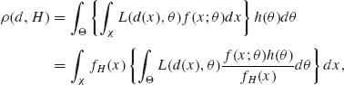
where fH(x) = ![]() f(x; τ) h(τ)dτ is the predictive p.d.f. The conditional p.d.f. h(θ | x) = f(x; θ)h(θ)/fH(x) is the posterior p.d.f. of θ, given X = x. Similarly, the conditional expectation
f(x; τ) h(τ)dτ is the predictive p.d.f. The conditional p.d.f. h(θ | x) = f(x; θ)h(θ)/fH(x) is the posterior p.d.f. of θ, given X = x. Similarly, the conditional expectation
(8.1.15) ![]()
is called the posterior risk of d(x) under H. Thus, for a given X = x, we can choose d(x) to minimize R(d(x), H). Since L(d(x), θ) ≥ 0 for all θ ![]() Θ and d
Θ and d ![]()
![]() , the minimization of the posterior risk minimizes also the prior risk ρ (d, H). Thus, dH(X) is a Bayes decision function.
, the minimization of the posterior risk minimizes also the prior risk ρ (d, H). Thus, dH(X) is a Bayes decision function.
8.2 BAYESIAN TESTING OF HYPOTHESIS
8.2.1 Testing Simple Hypothesis
We start with the problem of testing two simple hypotheses H0 and H1. Let F0(x) and F1(x) be two specified distribution functions. The hypothesis H0 specifies the parent distribution of X as F0(x), H1 specified it as F1(x). Let f0(x) and f1(x) be the p.d.f.s corresponding to F0(x) and F1(x), respectively. Let π, 0 ≤ π ≤ 1, be the prior probability that H0 is true. In the special case of two simple hypotheses, the loss function can assign 1 unit to the case of rejecting H0 when it is true and b units to the case of rejecting H1 when it is true. The prior risks associated with accepting H0 and H1 are, respectively, ρ0(π) = (1 − π)b and ρ1(π) = π. For a given value of π, we accept hypothesis Hi (i = 0, 1) if ρi(π) is the minimal prior risk. Thus, a Bayes rule, prior to making observations is
where d = i is the decision to accept Hi (i = 0, 1).
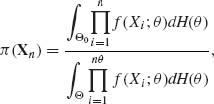
Suppose that a sample of n i.i.d. random variables X1, …, Xn has been observed. After observing the sample, we determine the posterior probability π (Xn) that H0 is true. This posterior probability is given by
(8.2.2) 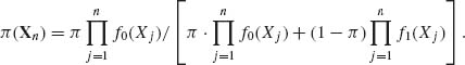
We use the decision rule (8.2.1) with π replaced by π(Xn). Thus, the Bayes decision function is
(8.2.3) 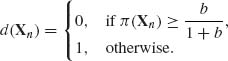
The Bayes decision function can be written in terms of the test function discussed in Chapter 4 as
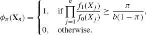
The Bayes test function ![]() π (Xn) is similar to the Neyman–Pearson most powerful test, except that the Bayes test is not necessarily randomized even if the distributions Fi(x) are discrete. Moreover, the likelihood ratio
π (Xn) is similar to the Neyman–Pearson most powerful test, except that the Bayes test is not necessarily randomized even if the distributions Fi(x) are discrete. Moreover, the likelihood ratio ![]() f1(Xj)/f0(Xj) is compared to the ratio of the prior risks.
f1(Xj)/f0(Xj) is compared to the ratio of the prior risks.
We discuss now some of the important optimality characteristics of Bayes tests of two simple hypotheses. Let R0(![]() ) and R1(
) and R1(![]() ) denote the risks associated with an arbitrary test statistic
) denote the risks associated with an arbitrary test statistic ![]() , when H0 or H1 are true, respectively. Let R0(π) and R1(π) denote the corresponding risk values of a Bayes test function, with respect to a prior probability π. Generally
, when H0 or H1 are true, respectively. Let R0(π) and R1(π) denote the corresponding risk values of a Bayes test function, with respect to a prior probability π. Generally
![]()
and
![]()
where ![]() 0(
0(![]() ) and
) and ![]() 1(
1(![]() ) are the error probabilities of the test statistic
) are the error probabilities of the test statistic ![]() , c1 and c2 are costs of erroneous decisions. The set R = {R0(
, c1 and c2 are costs of erroneous decisions. The set R = {R0(![]() ), R1(
), R1(![]() )); all test functions
)); all test functions ![]() } is called the risk set. Since for every 0 ≤ α ≤ 1 and any functions
} is called the risk set. Since for every 0 ≤ α ≤ 1 and any functions ![]() (1) and
(1) and ![]() (2), α
(2), α ![]() (1) + (1-α)
(1) + (1-α)![]() (2) is also a test function, and since
(2) is also a test function, and since
(8.2.5) ![]()
the risk set R is convex. Moreover, the set
(8.2.6) ![]()
of all risk points corresponding to the Bayes tests is the lower boundary for R. Indeed, according to (8.2.4) and the Neyman–Pearson Lemma, R1(π) is the smallest possible risk of all test functions ![]() with R0(
with R0(![]() ) = R0(π). Accordingly, all the Bayes tests constitute a complete class in the sense that, for any test function outside the class, there exists a corresponding Bayes test with a risk point having component smaller or equal to those of that particular test and at least one component is strictly smaller (Ferguson, 1967, Ch. 2). From the decision theoretic point of view there is no sense in considering test functions that do not belong to the complete class. These results can be generalized to the case of testing k simple hypotheses (Blackwell and Girshick, 1954; Ferguson, 1967).
) = R0(π). Accordingly, all the Bayes tests constitute a complete class in the sense that, for any test function outside the class, there exists a corresponding Bayes test with a risk point having component smaller or equal to those of that particular test and at least one component is strictly smaller (Ferguson, 1967, Ch. 2). From the decision theoretic point of view there is no sense in considering test functions that do not belong to the complete class. These results can be generalized to the case of testing k simple hypotheses (Blackwell and Girshick, 1954; Ferguson, 1967).
8.2.2 Testing Composite Hypotheses
Let Θ0 and Θ1 be the sets of θ–points corresponding to the (composite) hypotheses H0 and H1, respectively. These sets contain finite or infinite number of points. Let H(θ) be a prior distribution function specified over Θ = Θ0 ![]() Θ1. The posterior probability of H0, given n i.i.d. random variables X1, …, Xn, is
Θ1. The posterior probability of H0, given n i.i.d. random variables X1, …, Xn, is
where f(x; θ) is the p.d.f. of X under θ. The notation in (8.2.7) signifies that if the sets are discrete the corresponding integrals are sums and dH(θ) are prior probabilities, otherwise dH(θ) = h(θ)dθ, where h(θ) is a p.d.f. The Bayes decision rule is obtained by computing the posterior risk associated with accepting H0 or with accepting H1 and making the decision associated with the minimal posterior risk. The form of the Bayes test depends, therefore, on the loss function employed.
If the loss functions associated with accepting H0 or H1 are
![]()
then the associated posterior risk functions are
(8.2.8) ![]()
and
![]()
In this case, the Bayes test function is
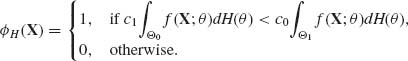
In other words, the hypothesis H0 is rejected if the predictive likelihood ratio
is greater than the loss ratio c1/c0. This can be considered as a generalization of (8.2.4). The predictive likelihood ratio ΛH(X) is called also the Bayes Factor in favor of H1 against H0 (Good, 1965, 1967).
Cornfield (1969) suggested as a test function the ratio of the posterior odds in favor of H0, i.e., P[H0| X]/(1 − P[H0| X]), to the prior odds π /(1 − π) where π = P[H0] is the prior probability of H0. The rule is to reject H0 when this ratio is smaller than a suitable constant. Cornfield called this statistic the relative betting odds. Note that this relative betting odds is [ΛH (X)π /(1 − π)]−1. We see that Cornfield’s test function is equivalent to (8.2.9) for suitably chosen cost factors.
Karlin (l956) and Karlin and Rubin (1956) proved that in monotone likelihood ratio families the Bayes test function is monotone in the sufficient statistic T(X). For testing H0: θ ≤ θ0 against H1: θ > θ0, the Bayes procedure rejects H0 whenever T(X) ≥ ξ0. The result can be further generalized to the problem of testing multiple hypotheses (Zacks, 1971; Ch. 10).
The problem of testing the composite hypothesis that all the probabilities in a multinomial distribution have the same value has drawn considerable attention in the statistical literature; see in particular the papers of Good (1967), Good and Crook (1974), and Good (1975). The Bayes test procedure proposed by Good (1967) is based on the symmetric Dirichlet prior distribution. More specifically if X = (X1, …, Xk)′ is a random vector having the multinomial distribution M(n, θ) then the parameter vector θ is ascribed the prior distribution with p.d.f.
(8.2.11) 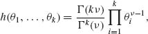
0 < θ1, …, θk < 1 and ![]() = 1. The Bayes factor for testing h0: θ =
= 1. The Bayes factor for testing h0: θ = ![]() 1 against the composite alternative hypothesis H1: θ ≠
1 against the composite alternative hypothesis H1: θ ≠ ![]() 1, where 1 = (1, …, 1)′, according to (8.2.10) is
1, where 1 = (1, …, 1)′, according to (8.2.10) is
(8.2.12) 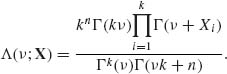
From the purely Bayesian point of view, the statistician should be able to choose an appropriate value of ν and some cost ratio c1/c0 for erroneous decisions, according to subjective judgment, and reject H0 if Λ (ν; X) ≥ c1/c0. In practice, it is generally not so simple to judge what are the appropriate values of ν and c1/c0. Good and Crook (1974) suggested two alternative ways to solve this problem. One suggestion is to consider an integrated Bayes factor
(8.2.13) ![]()
where ![]() (ν) is the p.d.f. of a log–Cauchy distribution, i.e.,
(ν) is the p.d.f. of a log–Cauchy distribution, i.e.,
(8.2.14) ![]()
The second suggestion is to find the value ν0 for which Λ (ν; X) is maximized and reject H0 if Λ* = (2log Λ (ν0; X))1/2 exceeds the (1 − α)–quantile of the asymptotic distribution of Λ* under H0. We see that non–Bayesian (frequentists) considerations are introduced in order to arrive at an appropriate critical level for Λ*. Good and Crook call this approach a “Bayes/Non–Bayes compromise.” We have presented this problem and the approaches suggested for its solution to show that in practical work a nondogmatic approach is needed. It may be reasonable to derive a test statistic in a Bayesian framework and apply it in a non–Bayesian manner.
8.2.3 Bayes Sequential Testing of Hypotheses
We consider in the present section an application of the general theory of Section 8.1.5 to the case of testing two simple hypotheses. We have seen in Section 8.2.1 that the Bayes decision test function, after observing Xn, is to reject H0 if the posterior probability, π(Xn), that H0 is true is less than or equal to a constant π*. The associated Bayes risk is ρ(0) (π (Xn)) = π (Xn)I{π (Xn) ≤ π* } + b(1 − π(Xn))I{π(Xn) > π* }, where π* = b/(1 + b). If π (Xn) = π then the posterior probability of H0 after the (n + 1)st observation is ![]() (π, Xn + 1) =
(π, Xn + 1) = ![]() , where R(x) =
, where R(x) = ![]() is the likelihood ratio. The predictive risk associated with an additional observation is
is the likelihood ratio. The predictive risk associated with an additional observation is
(8.2.15) ![]()
where c is the cost of one observation, and the expectation is with respect to the predictive distribution of X given π. We can show that the function ![]() 1(π) is concave on [0, 1] and thus continuous on (0, 1). Moreover,
1(π) is concave on [0, 1] and thus continuous on (0, 1). Moreover, ![]() 1(0) ≥ c and
1(0) ≥ c and ![]() 1(1) ≥ c. Note that the function
1(1) ≥ c. Note that the function ![]() (π, X) → 0 w.p.l if π → 0 and
(π, X) → 0 w.p.l if π → 0 and ![]() (π, X) → 1 w.p.l if π → 1. Since ρ(0)(π) is bounded by π*, we obtain by the Lebesgue Dominated Convergence Theorem that E{ρ0(
(π, X) → 1 w.p.l if π → 1. Since ρ(0)(π) is bounded by π*, we obtain by the Lebesgue Dominated Convergence Theorem that E{ρ0(![]() (π, X))} → 0 as π → 0 or as π → 1. The Bayes risk associated with an additional observation is
(π, X))} → 0 as π → 0 or as π → 1. The Bayes risk associated with an additional observation is
(8.2.16) ![]()
Thus, if c ≥ b/(1 + b) it is not optimal to make any observation. On the other hand, if c < b/(1 + b) there exist two points ![]() and
and ![]() , such that 0 <
, such that 0 < ![]() < π* <
< π* < ![]() < 1, and
< 1, and
(8.2.17) ![]()
Let
(8.2.18) ![]()
and let
(8.2.19) ![]()
Since ρ(1)(![]() (π, X)) ≤ ρ0(
(π, X)) ≤ ρ0(![]() (π, X)) for each π with probability one, we obtain that
(π, X)) for each π with probability one, we obtain that ![]() 2(π) ≤
2(π) ≤ ![]() 1(π) for all 0 ≤ π ≤ 1. Thus, ρ(2)(π) ≤ ρ(1)(π) for all π, 0 ≤ π ≤ 1.
1(π) for all 0 ≤ π ≤ 1. Thus, ρ(2)(π) ≤ ρ(1)(π) for all π, 0 ≤ π ≤ 1. ![]() 2(π) is also a concave function of π on [0, 1] and
2(π) is also a concave function of π on [0, 1] and ![]() 2(0) =
2(0) =![]() 2(1) = c. Thus, there exists
2(1) = c. Thus, there exists ![]() ≤
≤ ![]() and
and ![]() ≥
≥ ![]() such that
such that
(8.2.20) ![]()
We define now recursively, for each π on [0, 1],
(8.2.21) ![]()
and
(8.2.22) ![]()
These functions constitute for each π monotone sequences ![]() n(π) ≤
n(π) ≤ ![]() n−1 and ρ(n)(π) ≤ ρ(n−1) (π) for every n≥ 1. Moreover, for each n there exist 0 <
n−1 and ρ(n)(π) ≤ ρ(n−1) (π) for every n≥ 1. Moreover, for each n there exist 0 < ![]() ≤
≤ ![]() <
<![]() ≤
≤ ![]() < 1 such that
< 1 such that
(8.2.23) ![]()
Let ρ (π) = ![]() ρ(n)(π) for each π in [0, 1] and
ρ(n)(π) for each π in [0, 1] and ![]() (π) = E{ρ (
(π) = E{ρ (![]() (π, X))}. By the Lebesgue Monotone Convergence Theorem, we prove that
(π, X))}. By the Lebesgue Monotone Convergence Theorem, we prove that ![]() (π) =
(π) = ![]()
![]() n(π) for each π
n(π) for each π ![]() [0, 1]. The boundary points
[0, 1]. The boundary points ![]() and
and ![]() converge to π1 and π2, respectively, where 0 < π1 < π2 < 1. Consider now a nontruncated Bayes sequential procedure, with the stopping variable
converge to π1 and π2, respectively, where 0 < π1 < π2 < 1. Consider now a nontruncated Bayes sequential procedure, with the stopping variable
where X0 ≡ 0 and π (X0) ≡ π. Since under H0, π (Xn) → 1 with probability one and under H1, π (Xn) → 0 with probability 1, the stopping variable (8.2.24) is finite with probability one.
It is generally very difficult to determine the exact Bayes risk function ρ (π) and the exact boundary points π1 and π2. One can prove, however, that the Wald sequential probability ratio test (SPRT) (see Section 4.8.1) is a Bayes sequential procedure in the class of all stopping variables for which N≥ 1, corresponding to some prior probability π and cost parameter b. For a proof of this result, see Ghosh (1970, p. 93) or Zacks (1971, p. 456). A large sample approximation to the risk function ρ (π) was given by Chernoff (1959). Chernoff has shown that in the SPRT given by the boundaries (A, B) if A → −∞ and B → ∞, we have
(8.2.25) 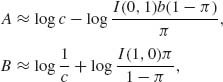
where the cost of observations c→ 0 and I(0, 1), I(1, 0) are the Kullback–Leibler information numbers. Moreover, as c→ 0
(8.2.26) ![]()
Shiryayev (1973, p. 127) derived an expression for the Bayes risk ρ (π) associated with a continuous version of the Bayes sequential procedure related to a Wiener process. Reduction of the testing problem for the mean of a normal distribution to a free boundary problem related to the Wiener process was done also by Chernoff (1961, 1965, 1968); see also the book of Dynkin and Yushkevich (1969).
A simpler sequential stopping rule for testing two simple hypotheses is
(8.2.27) ![]()
If π (XN) ≤ ![]() then H0 is rejected, and if π (XN) ≥ 1 −
then H0 is rejected, and if π (XN) ≥ 1 − ![]() then H0 is accepted. This stopping rule is equivalent to a Wald SPRT (A, B) with the limits
then H0 is accepted. This stopping rule is equivalent to a Wald SPRT (A, B) with the limits
![]()
If π = ![]() then, according to the results of Section 4.8.1, the average error probability is less than or equal to
then, according to the results of Section 4.8.1, the average error probability is less than or equal to ![]() . This result can be extended to the problem of testing k simple hypotheses (k≥ 2), as shown in the following.
. This result can be extended to the problem of testing k simple hypotheses (k≥ 2), as shown in the following.
Let H1, …, Hk be k hypotheses (k ≥ 2) concerning the distribution of a random variable (vector) X. According to Hj, the p.d.f. of X is fj(x; θ), θ![]() Θ j, j = 1, …, k. The parameter θ is a nuisance parameter, whose parameter space Θ j may depend on Hj. Let Gj(θ), j = 1, …, k, be a prior distribution on Θ j, and let π j be the prior probability that Hj is the true hypothesis,
Θ j, j = 1, …, k. The parameter θ is a nuisance parameter, whose parameter space Θ j may depend on Hj. Let Gj(θ), j = 1, …, k, be a prior distribution on Θ j, and let π j be the prior probability that Hj is the true hypothesis, ![]() π j = 1. Given n observations on X1, …, Xn, which are assumed to be conditionally i.i.d., we compute the predictive likelihood of Hj, namely,
π j = 1. Given n observations on X1, …, Xn, which are assumed to be conditionally i.i.d., we compute the predictive likelihood of Hj, namely,
(8.2.28) ![]()
j = 1, …, k. Finally, the posterior probability of Hj, after n observations, is
(8.2.29) 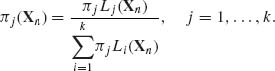
We consider the following Bayesian stopping variable, for some 0 < ![]() < 1.
< 1.
(8.2.30) ![]()
Obviously, one considers small values of ![]() , 0 <
, 0 < ![]() < 1/2, and for such
< 1/2, and for such ![]() , there is a unique value
, there is a unique value ![]() such that π
such that π ![]() (XN
(XN![]() ) ≥ 1 −
) ≥ 1 − ![]() . At stopping, hypothesis H
. At stopping, hypothesis H![]() is accepted.
is accepted.
For each n ≥ 1, partition the sample space ![]() (n) of Xn to (k + 1) disjoint sets
(n) of Xn to (k + 1) disjoint sets
![]()
and ![]() =
= ![]() n −
n − ![]()
![]() . As long as xn
. As long as xn ![]()
![]() we continue sampling. Thus, N
we continue sampling. Thus, N![]() = min
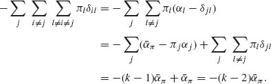
= min 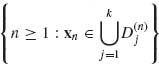 . In this sequential testing procedure, decision errors occur at stopping, when the wrong hypothesis is accepted. Thus, let δij denote the predictive probability of accepting Hi when Hj is the correct hypothesis. That is,
(8.2.31) ![]()
Note that, for π* = 1−![]() , πj(xn) ≥ π* if, and only if,
, πj(xn) ≥ π* if, and only if,
Let αj denote the predictive error probability of rejecting Hj when it is true, i.e., α j = ![]() δij.
δij.
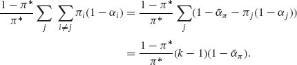
The average predictive error probability is ![]() π =
π = ![]() πjαj.
πjαj.
Theorem 8.2.1. For the stopping variable N![]() , the average predictive error probability is
, the average predictive error probability is ![]() π ≤
π ≤ ![]() .
.
Proof. From the inequality (8.2.32), we obtain
(8.2.33) 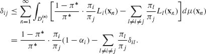
Summing over i, we get
![]()
or
![]()
Summing over j, we obtain
The first term on the RHS of (8.2.34) is
The second term on the RHS of (8.2.34) is
Substitution of (8.2.35) and (8.2.36) into (8.2.34) yields
![]()
or
![]() QED
QED
Thus, the Bayes sequential procedure given by the stopping variable N![]() and the associated decision rule can provide an excellent testing procedure when the number of hypothesis k is large. Rogatko and Zacks (1993) applied this procedure for testing the correct gene order. In this problem, if one wishes to order m gene loci on a chromosome, the number of hypotheses to test is k = m!/2.
and the associated decision rule can provide an excellent testing procedure when the number of hypothesis k is large. Rogatko and Zacks (1993) applied this procedure for testing the correct gene order. In this problem, if one wishes to order m gene loci on a chromosome, the number of hypotheses to test is k = m!/2.
8.3 BAYESIAN CREDIBILITY AND PREDICTION INTERVALS
8.3.1 Credibility Intervals
Let ![]() = {F(x; θ); θ
= {F(x; θ); θ ![]() Θ} be a parametric family of distribution functions. Let H(θ) be a specified prior distribution of θ and H(θ | X) be the corresponding posterior distribution, given X. If θ is real then an interval (Lα (X),
Θ} be a parametric family of distribution functions. Let H(θ) be a specified prior distribution of θ and H(θ | X) be the corresponding posterior distribution, given X. If θ is real then an interval (Lα (X), ![]() α (X)) is called a Bayes credibility interval of level 1 − α if for all X (with probability 1)
α (X)) is called a Bayes credibility interval of level 1 − α if for all X (with probability 1)
(8.3.1) ![]()
In multiparameter cases, we can speak of Bayes credibility regions. Bayes tolerance intervals are defined similarly.
Box and Tiao (1973) discuss Bayes intervals, called highest posterior density (HPD) intervals. These intervals are defined as θ intervals for which the posterior coverage probability is at least (1−α) and every θ–point within the interval has a posterior density not smaller than that of any θ–point outside the interval. More generally, a region RH(X) is called a (1 − α) HPD region if
The HPD intervals in cases of unimodal posterior distributions provide in nonsymmetric cases Bayes credibility intervals that are not equal tail ones. For various interesting examples, see Box and Tiao (1973).
8.3.2 Prediction Intervals
Suppose X is a random variable (vector) having a p.d.f. f(x;θ), θ ![]() Θ. If θ is known, an interval Iα (θ) is called a prediction interval for X, at level (1 − α) if
Θ. If θ is known, an interval Iα (θ) is called a prediction interval for X, at level (1 − α) if
(8.3.2) ![]()
When θ is unknown, one can use a Bayesian predictive distribution to determine an interval Iα (H) such that the predictive probability of {X![]() Iα (H)} is at least 1 − α. This predictive interval depends on the prior distribution H(θ). After observing X1, …, Xn, one can determine prediction interval (region) for (Xn+1, …, Xn+m) by using the posterior distribution H(θ| Xn) for the predictive distribution fH(x| xn) =
Iα (H)} is at least 1 − α. This predictive interval depends on the prior distribution H(θ). After observing X1, …, Xn, one can determine prediction interval (region) for (Xn+1, …, Xn+m) by using the posterior distribution H(θ| Xn) for the predictive distribution fH(x| xn) = ![]() f(x;θ) dH(θ| xn). In Example 8.12, we illustrate such prediction intervals. For additional theory and examples, see Geisser (1993).
f(x;θ) dH(θ| xn). In Example 8.12, we illustrate such prediction intervals. For additional theory and examples, see Geisser (1993).
8.4 BAYESIAN ESTIMATION
8.4.1 General Discussion and Examples
When the objective is to provide a point estimate of the parameter θ or a function ω = g(θ) we identify the action space with the parameter space. The decision function d(X) is an estimator with domain χ and range Θ, or Ω = g(Θ). For various loss functions the Bayes decision is an estimator ![]() H(X) that minimizes the posterior risk. In the following table, we present some loss functions and the corresponding Bayes estimators.
H(X) that minimizes the posterior risk. In the following table, we present some loss functions and the corresponding Bayes estimators.
In the examples, we derived Bayesian estimators for several models of interest, and show the dependence of the resulting estimators on the loss function and on the prior distributions.
| Loss Function | Bayes Estimator |
| ( |
|
| (The posterior expectation) | |
| Q(θ)( |
EH{θ Q(θ)| X} /EH{Q(θ)| X} |
| | |
|
| distribution, i.e., H−1(.5| X). | |
| a( |
The |
| i.e., H−1( |
8.4.2 Hierarchical Models
Lindley and Smith (1972) and Smith (1973a, b) advocated a somewhat more complicated methodology. They argue that the choice of a proper prior should be based on the notion of exchangeability. Random variables W1, W2, …, Wk are called exchangeable if the joint distribution of (W1, …, Wk) is the same as that of (Wi1, …, Wik), where (i1, …, ik) is any permutation of (1, 2, …, k). The joint p.d.f. of exchangeable random variables can be represented as a mixture of appropriate p.d.f.s of i.i.d. random variables. More specifically, if, conditional on w, W1, …, Wk are i.i.d. with p.d.f. f(W1, …, Wk;w) = ![]() g(Wi, w), and if w is given a probability distribution P(w) then the p.d.f.
g(Wi, w), and if w is given a probability distribution P(w) then the p.d.f.
(8.4.1) 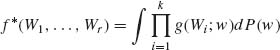
represents a distribution of exchangeable random variables. If the vector X represents the means of k independent samples the present model coincides with the Model II of ANOVA, with known variance components and an unknown grand mean μ. This model is a special case of a Bayesian linear model called by Lindley and Smith a three–stage linear model or hierarchical models. The general formulation of such a model is
![]()
and
![]()
where X is an n × 1 vector, θi are pi × 1 (i = 1, 2, 3), A1, A2, A3 are known constant matrices, and V, ![]() , C are known covariance matrices. Lindley and Smith (1972) have shown that for a noninformative prior for θ2 obtained by letting C−1 → 0, the Bayes estimator of θ, for the loss function L(
, C are known covariance matrices. Lindley and Smith (1972) have shown that for a noninformative prior for θ2 obtained by letting C−1 → 0, the Bayes estimator of θ, for the loss function L(![]() 1, θ) = ||
1, θ) = ||![]() 1 − θ1||2, is given by
1 − θ1||2, is given by
(8.4.2) ![]()
where
(8.4.3) ![]()
We see that this Bayes estimator coincides with the LSE, (A′A)−1A′X, when V = I and ![]() ,−1→ 0. This result depends very strongly on the knowledge of the covariance matrix V. Lindley and Smith (1972) suggested an iterative solution for a Bayesian analysis when V is unknown. Interesting special results for models of one way and two–way ANOVA can be found in Smith (1973b).
,−1→ 0. This result depends very strongly on the knowledge of the covariance matrix V. Lindley and Smith (1972) suggested an iterative solution for a Bayesian analysis when V is unknown. Interesting special results for models of one way and two–way ANOVA can be found in Smith (1973b).
A comprehensive Bayesian analysis of the hierarchical Model II of ANOVA is given in Chapter 5 of Box and Tiao (1973).
In Gelman et al. (1995, pp. 129–134), we find an interesting example of a hierarchical model in which
![]()
θ1, …, θk are conditionally i.i.d., with
![]()
and (α, β) have an improper prior p.d.f.
![]()
According to this model, θ = (θ1, …, θ k) is a vector of priorly exchangeable (not independent) parameters. We can easily show that the posterior joint p.d.f. of θ, given J = (J1, …, Jk) and (α, β) is
(8.4.4) 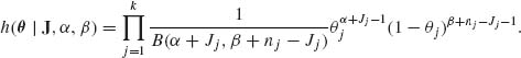
In addition, the posterior p.d.f. of (α, β) is
(8.4.5) 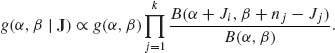
The objective is to obtain the joint posterior p.d.f.

From h(θ| J) one can derive a credibility region for θ, etc.
8.4.3 The Normal Dynamic Linear Model
In time–series analysis for econometrics, signal processing in engineering and other areas of applications, one often encounters series of random vectors that are related according to the following linear dynamic model
where A and G are known matrices, which are (for simplicity) fixed. {![]() n} is a sequence of i.i.d. random vectors; {ωn} is a sequence of i.i.d. random vectors; {
n} is a sequence of i.i.d. random vectors; {ωn} is a sequence of i.i.d. random vectors; {![]() n} and {ωn} are independent sequences, and
n} and {ωn} are independent sequences, and
(8.4.7) ![]()
We further assume that θ0 has a prior normal distribution, i.e.,
(8.4.8) ![]()
and that θ0 is independent of {![]() t} and {ω t}. This model is called the normal random walk model.
t} and {ω t}. This model is called the normal random walk model.
We compute now the posterior distribution of θ1, given Y1. From multivariate normal theory, since
![]()
and
![]()
we obtain
![]()
Let F1 = Ω + GC0G′. Then, we obtain after some manipulations
![]()
where
(8.4.9) ![]()
and
(8.4.10) ![]()
Define, recursively for j ≥ 1
![]()
and
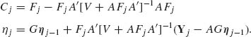
The recursive equations (8.4.11) are called the Kalman filter. Note that, for each n ≥ 1, ηn depends on ![]() n = (Y1, …, Yn). Moreover, we can prove by induction on n, that
n = (Y1, …, Yn). Moreover, we can prove by induction on n, that
(8.4.12) ![]()
for all n ≥ 1. For additional theory and applications in Bayesian forecasting and smoothing, see Harrison and Stevens (1976), West, Harrison, and Migon (1985), and the book of West and Harrison (1997). We illustrate this sequential Bayesian process in Example 8.19.
8.5 APPROXIMATION METHODS
In this section, we discuss two types of methods to approximate posterior distributions and posterior expectations. The first type is analytical, which is usually effective in large samples. The second type of approximation is numerical. The numerical approximations are based either on numerical integration or on simulations. Approximations are required when an exact functional form for the factor of proportionality in the posterior density is not available. We have seen such examples earlier, like the posterior p.d.f. (8.1.4).
8.5.1 Analytical Approximations
The analytic approximations are saddle–point approximations, based on variations of the Laplace method, which is explained now.
Consider the problem of evaluating the integral
where θ is m–dimensional, and k(θ) has sufficiently high–order continuous partial derivatives. Consider first the case of m = 1. Let ![]() be an argument maximizing −k(θ). Make a Taylor expansion of k(θ) around
be an argument maximizing −k(θ). Make a Taylor expansion of k(θ) around ![]() , i.e.,
, i.e.,
k′(![]() ) = 0 and k″(
) = 0 and k″(![]() ) > 0. Thus, substituting (8.5.2) in (8.5.1), the integral I is approximated by
) > 0. Thus, substituting (8.5.2) in (8.5.1), the integral I is approximated by
(8.5.3) 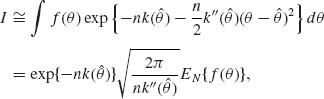
where EN{f(θ)} is the expected value of f(θ), with respect to the normal distribution with mean ![]() and variance
and variance ![]() . The expectation EN{f(θ)} can be sometimes computed exactly, or one can apply the delta method to obtain the approximation
. The expectation EN{f(θ)} can be sometimes computed exactly, or one can apply the delta method to obtain the approximation
(8.5.4) ![]()
Often we see the simpler approximation, in which f(![]() ) is used for EN{f(
) is used for EN{f(![]() )}. In this case, the approximation error is O(n−1). If we use f(
)}. In this case, the approximation error is O(n−1). If we use f(![]() ) for EN{f(θ)}, we obtain the approximation
) for EN{f(θ)}, we obtain the approximation
(8.5.5) 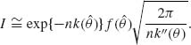
In the m > 1 case, the approximating formula becomes
(8.5.6) ![]()
where
(8.5.7) ![]()
These approximating formulae can be applied in Bayesian analysis, by letting −nk(θ) be the log–likelihood function, l(θ* | Xn); ![]() be the MLE,
be the MLE, ![]() n, and
n, and ![]() , −1(
, −1(![]() ) be J(
) be J(![]() n) given in (7.7.15). Accordingly, the posterior p.d.f., when the prior p.d.f. is h(θ), is approximated by
n) given in (7.7.15). Accordingly, the posterior p.d.f., when the prior p.d.f. is h(θ), is approximated by
(8.5.8) ![]()
In this formula, ![]() n is the MLE of θ and
n is the MLE of θ and
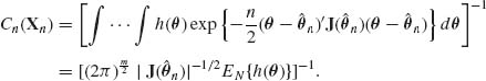
If we approximate EN{h(θ)} by h(![]() n), then the approximating formula reduces to
n), then the approximating formula reduces to
(8.5.10) ![]()
This is a large sample normal approximation to the posterior density of θ. We can write this, for large samples, as
Note that Equation (8.5.11) does not depend on the prior distribution, and is not expected therefore to yield good approximation to h(θ| Xn) if the samples are not very large.
One can improve upon the normal approximation (8.5.11) by combining the likelihood function and the prior density h(θ) in the definition of k(θ). Thus, let
(8.5.12) ![]()
Let ![]() be a value of θ maximizing −n
be a value of θ maximizing −n ![]() (θ), or
(θ), or ![]() n the root of
n the root of
(8.5.13) ![]()
Let
(8.5.14) ![]()
Then, the saddle–point approximation to the posterior p.d.f. h(θ | Xn) is
This formula is similar to Barndorff–Nielsen p*–formula (7.7.15) and reduces to the p*–formula if h(θ)dθ ![]() dθ. The normal approximation is given by (8.5.11), in which
dθ. The normal approximation is given by (8.5.11), in which ![]() n is replaced by
n is replaced by ![]() n and J(
n and J(![]() n) is replaced by
n) is replaced by ![]() (
(![]() n).
n).
For additional reading on analytic approximation for large samples, see Gamerman (1997, Ch. 3), Reid (1995, pp. 351–368), and Tierney and Kadane (1986).
8.5.2 Numerical Approximations
In this section, we discuss two types of numerical approximations: numerical integrations and simulations. The reader is referred to Evans and Swartz (2001).
I. Numerical Integrations
We have seen in the previous sections that, in order to evaluate posterior p.d.f., one has to evaluate integrals of the form
Sometimes these integrals are quite complicated, like that of the RHS of Equa-tion (8.1.4).
Suppose that, as in (8.5.16), the range of integration is from −∞ to ∞ and I < ∞. Consider first the case where θ is real. Making the one–to–one transformation ω = eθ /(1+eθ), the integral of (8.5.16) is reduced to
where q(θ) = L(θ | Xn)h(θ). There are many different methods of numerical integration. A summary of various methods and their accuracy is given in Abramowitz and Stegun (1968, p. 885). The reader is referred also to the book of Davis and Rabinowitz (1984).
If we define f(ω) so that
(8.5.18) ![]()
then, an n–point approximation to I is given by
where
(8.5.20) 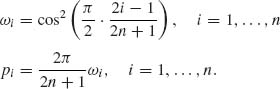
The error in this approximation is
(8.5.21) ![]()
Integrals of the form
Thus, (8.5.22) can be computed according to (8.5.19). Another method is to use an n–points Gaussian quadrature formula:
where ui and wi are tabulated in Table 25.4 of Abramowitz and Stegun (1968, p. 916). Often it suffices to use n = 8 or n = 12 points in (8.5.23).
II. Simulation
The basic theorem applied in simulations to compute an integral I = ![]() f(θ) dH(θ) is the strong law of large numbers (SLLN). We have seen in Chapter 1 that if X1, X2, … is a sequence of i.i.d. random variables having a distribution FX(x), and if
f(θ) dH(θ) is the strong law of large numbers (SLLN). We have seen in Chapter 1 that if X1, X2, … is a sequence of i.i.d. random variables having a distribution FX(x), and if ![]() |g(x)|dF(x) < ∞ then
|g(x)|dF(x) < ∞ then
![]()
This important result is applied to approximate an integral ![]() f(θ)dH(θ) by a sequence θ1, θ2, … of i.i.d. random variables, generated from the prior distribution H(θ). Thus, for large n,
f(θ)dH(θ) by a sequence θ1, θ2, … of i.i.d. random variables, generated from the prior distribution H(θ). Thus, for large n,
(8.5.24) ![]()
Computer programs are available in all statistical packages that simulate realizations of a sequence of i.i.d. random variables, having specified distributions. All programs use linear congruential generators to generate “pseudo” random numbers that have approximately uniform distribution on (0, 1). For discussion of these generators, see Bratley, Fox, and Schrage (1983).
Having generated i.i.d. uniform R(0, 1) random variables U1, U2, …, Un, one can obtain a simulation of i.i.d. random variables having a specific c.d.f. F, by the transformation
(8.5.25) ![]()
In some special cases, one can use different transformations. For example, if U1, U2 are independent R(0, 1) random variables then the Box–Muller transformation
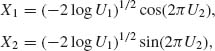
yields two independent random variables having a standard normal distribution. It is easier to simulate a N(0, 1) random variable according to (8.5.26) than according to X =Φ −1(U). In today’s technology, one could choose from a rich menu of simulation procedures for many of the common distributions.
If a prior distribution H(θ) is not in a simulation menu, or if h(θ)dθ is not proper, one can approximate ![]() f(θ)h(θ)dθ by generating θ1, …, θn from another convenient distribution, λ (θ)dθ say, and using the formula
f(θ)h(θ)dθ by generating θ1, …, θn from another convenient distribution, λ (θ)dθ say, and using the formula
(8.5.27) ![]()
The method of simulating from a substitute p.d.f. λ (θ) is called importance sampling, and λ (θ) is called an importance density. The choice of λ (θ) should follow the following guidelines:
The second guideline is sometimes complicated. For example, if h(θ) d(θ) is the improper prior dθ and I = ![]() f(θ)dθ, where
f(θ)dθ, where ![]() |f(θ)|dθ < ∞, one could use first the monotone transformation x = eθ /(1+eθ) to reduce I to I =
|f(θ)|dθ < ∞, one could use first the monotone transformation x = eθ /(1+eθ) to reduce I to I = ![]() . One can use then a beta, β (p, q), importance density to simulate from, and approximate I by
. One can use then a beta, β (p, q), importance density to simulate from, and approximate I by
![]()
It would be simpler to use β (1, 1), which is the uniform R(0, 1).
An important question is, how large should the simulation sample be, so that the approximation will be sufficiently precise. For large values of n, the approximation ![]() f(θi) h(θi) is, by Central Limit Theorem, approximately distributed like
f(θi) h(θi) is, by Central Limit Theorem, approximately distributed like ![]() , where
, where
![]()
VS(·) is the variance according to the simulation density. Thus, n could be chosen sufficiently large, so that Z1−α /2 · ![]() < δ. This will guarantee that with confidence probability close to (1 − α) the true value of I is within
< δ. This will guarantee that with confidence probability close to (1 − α) the true value of I is within ![]() ± δ. The problem, however, is that generally τ2 is not simple or is unknown. To overcome this problem one could use a sequential sampling procedure, which attains asymptotically the fixed width confidence interval. Such a procedure was discussed in Section 6.7.
± δ. The problem, however, is that generally τ2 is not simple or is unknown. To overcome this problem one could use a sequential sampling procedure, which attains asymptotically the fixed width confidence interval. Such a procedure was discussed in Section 6.7.
We should remark in this connection that simulation results are less accurate than those of numerical integration. One should use, as far as possible, numerical integration rather than simulation.
To illustrate this point, suppose that we wish to compute numerically
![]()
Reduce I, as in (8.5.17), to
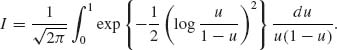
Simulation of N = 10, 000 random variables Ui ∼ R(0, 1) yields the approximation
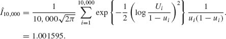
On the other hand, a 10–point numerical integration, according to (8.5.29), yields
![]()
When θ is m–dimensional, m ≥ 2, numerical integration might become too difficult. In such cases, simulations might be the answer.
8.6 EMPIRICAL BAYES ESTIMATORS
Empirical Bayes estimators were introduced by Robbins (1956) for cases of repetitive estimation under similar conditions, when Bayes estimators are desired but the statistician does not wish to make specific assumptions about the prior distribution. The following example illustrates this approach. Suppose that X has a Poisson distribution P(λ), and λ has some prior distribution H(λ), 0 < λ < ∞. The Bayes estimator of λ for the squared–error loss function is
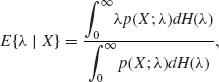
where p(x;λ) denotes the p.d.f. of P(λ) at the point x. Since λ p(x;λ) = (x + 1)· p(x + 1;λ) for every λ and each x = 0, 1, … we can express the above Bayes estimator in the form
(8.6.1) 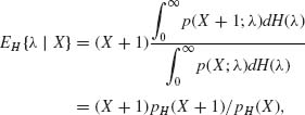
where pH(x) is the predictive p.d.f. at x. Obviously, in order to determine the posterior expectation we have to know the prior distribution H(λ). On the other hand, if the problem is repetitive in the sense that a sequence (X1, λ1), (X2, λ2), …, (Xn, λn), …, is generated independently so that λ1, λ2, … are i.i.d. having the same prior distribution H(λ), and X1, …, Xn are conditionally independent, given λ1, …, λn, then we consider the sequence of observable random variables X1, …, Xn, … as i.i.d. from the mixture of Poisson distribution with p.d.f. pH(j), j = 0, 1, 2, …. Thus, if on the nth epoch, we observe Xn = i0 we estimate, on the basis of all the data, the value of pH(i0 + 1)/pH(i0). A consistent estimator of pH(j), for any j = 0, 1, … is ![]() , where I{Xi = j} is the indicator function of {Xi = j}. This follows from the SLLN. Thus, a consistent estimator of the Bayes estimator EH{λ | Xn} is
, where I{Xi = j} is the indicator function of {Xi = j}. This follows from the SLLN. Thus, a consistent estimator of the Bayes estimator EH{λ | Xn} is
(8.6.2) 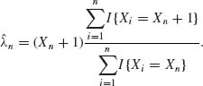
This estimator is independent of the unknown H(λ), and for large values of n is approximately equal to EH{λ | Xn}. The estimator ![]() n is called an empirical Bayes estimator. The question is whether the prior risks, under the true H(λ), of the estimators λn converge, as n → ∞, to the Bayes risk under H(λ). A general discussion of this issue with sufficient conditions for such convergence of the associated prior risks is given in the paper of Robbins (1964).
n is called an empirical Bayes estimator. The question is whether the prior risks, under the true H(λ), of the estimators λn converge, as n → ∞, to the Bayes risk under H(λ). A general discussion of this issue with sufficient conditions for such convergence of the associated prior risks is given in the paper of Robbins (1964).
Many papers were written on the application of the empirical Bayes estimation method to repetitive estimation problems in which it is difficult or impossible to specify the prior distribution exactly. We have to remark in this connection that the empirical Bayes estimators are only asymptotically optimal. We have an adaptive decision process which corrects itself and approaches the optimal decisions only when n grows. How fast does it approach the optimal decisions? It depends on the amount of a priori knowledge of the true prior distribution. The initial estimators may be far from the true Bayes estimators. A few studies have been conducted to estimate the rate of approach of the prior risks associated with the empirical Bayes decisions to the true Bayes risk. Lin (1974) considered the one parameter exponential family and the estimation of a function λ (θ) under squared–error loss. The true Bayes estimator is
![]()
and it is assumed that ![]() (x)fH(x) can be expressed in the form
(x)fH(x) can be expressed in the form ![]() , where
, where ![]() is the ith order derivative of fH(x) with respect to x. The empirical Bayes estimators considered are based on consistent estimators of the p.d.f. fH(x) and its derivatives. For the particular estimators suggested it is shown that the rate of approach is of the order 0(n–α) with 0 < α ≤ 1/3, where n is the number of observations.
is the ith order derivative of fH(x) with respect to x. The empirical Bayes estimators considered are based on consistent estimators of the p.d.f. fH(x) and its derivatives. For the particular estimators suggested it is shown that the rate of approach is of the order 0(n–α) with 0 < α ≤ 1/3, where n is the number of observations.
In Example 8.26, we show that if the form of the prior is known, the rate of approach becomes considerably faster. When the form of the prior distribution is known the estimators are called semi–empirical Bayes, or parametric empirical Bayes.
For further reading on the empirical Bayes method, see the book of Maritz (1970) and the papers of Casella (1985), Efron and Morris (1971, l972a, 1972b), and Susarla (1982).
The E–M algorithm discussed in Example 8.27 is a very important procedure for estimation and overcoming problems of missing values. The book by McLachlan and Krishnan (1997) provides the theory and many interesting examples.
PART II: EXAMPLES
Example 8.1. The experiment under consideration is to produce concrete under certain conditions of mixing the ingredients, temperature of the air, humidity, etc. Prior experience shows that concrete cubes manufactured in that manner will have a compressive strength X after 3 days of hardening, which has a log–normal distribution LN(μ, σ2). Furthermore, it is expected that 95% of such concrete cubes will have compressive strength in the range of 216–264 (kg/cm2).
According to our model, Y = log X ∼ N(μ, σ2). Taking the (natural) logarithms of the range limits, we expect most Y values to be within the interval (5.375, 5.580).
The conditional distribution of Y given (μ, σ2) is
![]()
Suppose that σ2 is fixed at σ2 = 0.001, and μ has a prior normal distribution μ ∼ N(μ0, τ2), then the predictive distribution of Y is N(μ0, σ2 + τ2). Substituting μ0 = 5.475, the predictive probability that Y ![]() (5.375, 5.580), if
(5.375, 5.580), if ![]() = 0.051 is 0.95. Thus, we choose τ2 = 0.0015 for the prior distribution of μ.
= 0.051 is 0.95. Thus, we choose τ2 = 0.0015 for the prior distribution of μ.
From this model of Y | μ, σ2 ∼ N(μ, σ2) and μ ∼ N(μ0, τ2). The bivariate distribution of (Y, μ) is
![]()
Hence, the conditional distribution of μ given {Y = y} is, as shown in Section 2.9,
![]()
The posterior distribution of μ, given {Y = y} is normal. ![]()
Example 8.2. (a) X1, X2, …, Xn given λ are conditionally i.i.d., having a Poisson distribution P(λ), i.e., ![]() = {P(λ), 0 < λ < ∞}.
= {P(λ), 0 < λ < ∞}.
Let ![]() = {G(Λ, α), 0 < α, Λ < ∞}, i.e.,
= {G(Λ, α), 0 < α, Λ < ∞}, i.e., ![]() is a family of prior gamma distributions for λ. The minimal sufficient statistics, given λ, is
is a family of prior gamma distributions for λ. The minimal sufficient statistics, given λ, is ![]() . Tn| λ ∼ P(λ n). Thus, the posterior p.d.f. of λ, given Tn, is
. Tn| λ ∼ P(λ n). Thus, the posterior p.d.f. of λ, given Tn, is
![]()
Hence, λ | Tn ∼ G(n + Λ, Tn + α). The posterior distribution belongs to ![]() .
.
(b) ![]() = {G(λ, α), 0 < λ < ∞}, α fixed.
= {G(λ, α), 0 < λ < ∞}, α fixed. ![]() = {G(Λ, ν), 0 < ν, Λ < ∞}.
= {G(Λ, ν), 0 < ν, Λ < ∞}.
![]()
Thus, λ | X ∼ G(X + Λ, ν + α). ![]()
Example 8.3. The following problem is often encountered in high technology industry.
The number of soldering points on a typical printed circut board (PCB) is often very large. There is an automated soldering technology, called “wave soldering, ” which involves a large number of different factors (conditions) represented by variables X1, X2, …, Xk. Let J denote the number of faults in the soldering points on a PCB. One can model J as having conditional Poisson distribution with mean λ, which depends on the manufacturing conditions X1, …, Xk according to a log–linear relationship
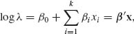
where β′ = (β0, …, βk) and x = (1, x1, …, xk). β is generally an unknown parametric vector. In order to estimate β, one can design an experiment in which the values of the control variables X1, …, Xk are changed.
Let Ji be the number of observed faulty soldering points on a PCB, under control conditions given by xi (i = 1, …, N). The likelihood function of β, given J1, …, JN and x1, …, xN, is
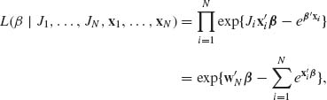
where ![]() . If we ascribe β a prior multinormal distribution, i.e., β ∼ N(β0, V) then the posterior p.d.f. of β, given
. If we ascribe β a prior multinormal distribution, i.e., β ∼ N(β0, V) then the posterior p.d.f. of β, given ![]() N = (J1, …, JN, x1, …, xN), is
N = (J1, …, JN, x1, …, xN), is
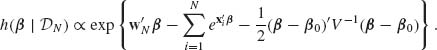
It is very difficult to express analytically the proportionality factor, even in special cases, to make the RHS of h(β| ![]() N)a p.d.f.
N)a p.d.f. ![]()
Example 8.4. In this example, we derive the Jeffreys prior density for several models.
A. ![]() = {b(x;n, θ), 0 < θ < 1}.
= {b(x;n, θ), 0 < θ < 1}.
This is the family of binomial probability distributions. The Fisher information function is
![]()
Thus, the Jeffreys prior for θ is
![]()
In this case, the prior density is
![]()
This is a proper prior density. The posterior distribution of θ, given X, under the above prior is Beta ![]() .
.
B. ![]() = {N(μ, σ2);−∞ < μ < ∞, 0 < σ < ∞}.
= {N(μ, σ2);−∞ < μ < ∞, 0 < σ < ∞}.
The Fisher information matrix is given in (3.8.8). The determinant of this matrix is |I(μ, σ2)| = 1/2σ6. Thus, the Jeffreys prior for this model is
![]()
Using this improper prior density the posterior p.d.f. of (μ, σ2), given X1, …, Xn, is
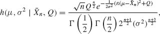
where ![]() . The parameter
. The parameter ![]() is called the precision parameter. In terms of μ and
is called the precision parameter. In terms of μ and ![]() , the improper prior density is
, the improper prior density is
![]()
The posterior density of (μ, ![]() ) correspondingly is
) correspondingly is
![]()
Example 8.5. Consider a simple inventory system in which a certain commodity is stocked at the beginning of every day, according to a policy determined by the following considerations. The daily demand (in number of units) is a random variable X whose distribution belongs to a specified parametric family ![]() . Let X1, X2, … denote a sequence of i.i.d. random variables, whose common distribution F(x;θ) belongs to
. Let X1, X2, … denote a sequence of i.i.d. random variables, whose common distribution F(x;θ) belongs to ![]() and which represent the observed demand on consecutive days. The stock level at the beginning of each day, Sn, n = 1, 2, … can be adjusted by increasing or decreasing the available stock at the end of the previous day. We consider the following inventory cost function
and which represent the observed demand on consecutive days. The stock level at the beginning of each day, Sn, n = 1, 2, … can be adjusted by increasing or decreasing the available stock at the end of the previous day. We consider the following inventory cost function
![]()
where c, 0 < c < ∞, is the daily cost of holding a unit in stock and h, 0 < h < ∞ is the cost (or penalty) for a shortage of one unit. Here (s − x)+ = max(0, s − x) and (s − x)- = -min(0, s − x). If the distribution of X, F(x;θ) is known, then the expected cost R(S, θ) = Eθ {K(S, X)} is minimized by
![]()
where F-1(γ ;θ) is the γ–quantile of F(x;θ). If θ is unknown we cannot determine S0(θ). We show now a Bayesian approach to the determination of the stock levels. Let H(θ) be a specific prior distribution of θ. The prior expected daily cost is
![]()
or, since all the terms are nonnegative

The value of S which minimizes ρ (S, H) is similar to (8.1.27),
![]()
i.e., the h/(c + h) th–quantile of the predictive distribution FH(x).
After observing the value x1 of X1, we convert the prior distribution H(θ) to a posterior distribution H1(θ | x1) and determine the predictive p.d.f. for the second day, namely
![]()
The expected cost for the second day is
Moreover, by the law of the iterated expectations
![]()
Hence,
The conditional expectation  is the posterior expected cost given X1 = x; or the predictive cost for the second day. The optimal choice of S2 given X1 = x is, therefore, the h/(c + h)–quantile of the predictive distribution FH1(y | x) i.e.,
 ![]() . Since this function minimizes the predictive risk for every x, it minimizes ρ(S2, H). In the same manner, we prove that after n days, given Xn = (x1, …, xn) the optimal stock level for the beginning of the (n + 1)st day is the
. Since this function minimizes the predictive risk for every x, it minimizes ρ(S2, H). In the same manner, we prove that after n days, given Xn = (x1, …, xn) the optimal stock level for the beginning of the (n + 1)st day is the ![]() –quantile of the predictive distribution of Xn + 1, given Xn = xn, i.e.,
–quantile of the predictive distribution of Xn + 1, given Xn = xn, i.e., ![]() , where the predictive p.d.f. of Xn + 1, given Xn = x is
, where the predictive p.d.f. of Xn + 1, given Xn = x is
![]()
and h(θ | x) is the posterior p.d.f. of θ given Xn = x. The optimal stock levels are determined sequentially for each day on the basis of the demand of the previous days. Such a procedure is called an adaptive procedure. In particular, if X1, X2, … is a sequence of i.i.d. Poisson random variables (r.v.s), P(θ) and if the prior distribution H(θ) is the gamma distribution, ![]() , the posterior distribution of θ after n observations is the gamma distribution
, the posterior distribution of θ after n observations is the gamma distribution ![]() , where
, where ![]() . Let
. Let ![]() denote the p.d.f. of this posterior distribution. The predictive distribution of Xn + 1 given Xn, which actually depends only on Tn, is
denote the p.d.f. of this posterior distribution. The predictive distribution of Xn + 1 given Xn, which actually depends only on Tn, is
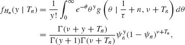
where ![]() n = τ/(1 + (n + 1)τ). This is the p.d.f. of the negative binomial NB(
n = τ/(1 + (n + 1)τ). This is the p.d.f. of the negative binomial NB(![]() n, ν + Tn). It is interesting that in the present case the predictive distribution belongs to the family of the negative–binomial distributions for all n = 1, 2, …. We can also include the case of n = 0 by defining T0 = 0. What changes from one day to another are the parameters (
n, ν + Tn). It is interesting that in the present case the predictive distribution belongs to the family of the negative–binomial distributions for all n = 1, 2, …. We can also include the case of n = 0 by defining T0 = 0. What changes from one day to another are the parameters (![]() n, ν + Tn). Thus, the optimal stock level at the beginning of the (n + 1)st day is the h/(c + h)–quantile of the NB(
n, ν + Tn). Thus, the optimal stock level at the beginning of the (n + 1)st day is the h/(c + h)–quantile of the NB(![]() n, ν + Tn).
n, ν + Tn). ![]()
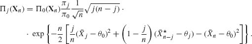
Example 8.6. Consider the testing problem connected with the problem of detecting disturbances in a manufacturing process. Suppose that the quality of a product is presented by a random variable X having a normal distribution N(θ, 1). When the manufacturing process is under control the value of θ should be θ0. Every hour an observation is taken on a product chosen at random from the process. Consider the situation after n hours. Let X1, …, Xn be independent random variables representing the n observations. It is suspected that after k hours of operation 1 < k < n a malfunctioning occurred and the expected value θ shifted to a value θ1 greater than θ0. The loss due to such a shift is (θ1 – θ0) [$] per hour. If a shift really occurred the process should be stopped and rectified. On the other hand, if a shift has not occurred and the process is stopped a loss of K [$] is charged. The prior probability that the shift occurred is ![]() . We present here the Bayes test of the two hypotheses
. We present here the Bayes test of the two hypotheses
![]()
against
![]()
for a specified k, 1 ≤ k ≤ n − 1; which is performed after the nth observation.
The likelihood functions under H0 and under H1 are, respectively, when Xn = xn
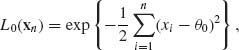
and
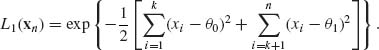
Thus, the posterior probability that H0 is true is
![]()
where π = 1 –![]() . The ratio of prior risks is in the present case K π/((1-π)(n − k)(θ1 – θ0)). The Bayes test implies that H0 should be rejected if
. The ratio of prior risks is in the present case K π/((1-π)(n − k)(θ1 – θ0)). The Bayes test implies that H0 should be rejected if
![]()
where 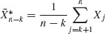 .
.
The Bayes (minimal prior) risk associated with this test is
![]()
where ![]() 0(π) and
0(π) and ![]() 1(π) are the error probabilities of rejecting H0 or H1 when they are true. These error probabilities are given by
1(π) are the error probabilities of rejecting H0 or H1 when they are true. These error probabilities are given by
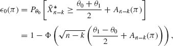
where Φ(z) is the standard normal integral and
![]()
Similarly,
![]()
The function An − k(π) is monotone increasing in π and ![]() . Accordingly,
. Accordingly, ![]() 0(0) = 1,
0(0) = 1, ![]() 1(0) = 0 and
1(0) = 0 and ![]() 0(1) = 0,
0(1) = 0, ![]() 1(1) = 1.
1(1) = 1. ![]()
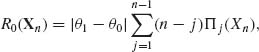
Example 8.7. Consider the detection problem of Example 8.6 but now the point of shift k is unknown. If θ0 and θ1 are known then we have a problem of testing the simple hypothesis H0 (of Example 8.6) against the composite hypothesis
![]()
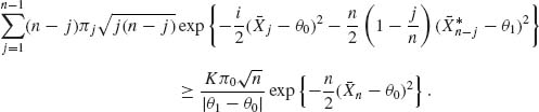
Let π0 be the prior probability of H0 and πj, j = 1, …, n − 1, the prior probabilities under H1 that {k = j}. The posterior probability of H0 is then
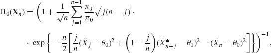
where 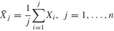 and
and 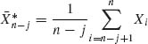 . The posterior probability of {k = j} is, for j = 1, …, n − 1,
Let Ri(Xn) (i = 0, 1) denote the posterior risk associated with accepting Hi. These functions are given by
and
![]()
H0 is rejected if R1(Xn) ≤ R0(Xn), or when
![]()
Example 8.8. We consider here the problem of testing whether the mean of a normal distribution is negative or positive. Let X1, …, Xn be i.i.d. random variables having a N(θ, 1) distribution. The null hypothesis is H0: θ ≤ 0 and the alternative hypothesis is H1: θ > 0. We assign the unknown θ a prior normal distribution, i.e., θ ∼ N(0, τ2). Thus, the prior probability of H0 is π = ![]() . The loss function L0(θ) of accepting H0 and that of accepting H1, L1(θ), are of the form
. The loss function L0(θ) of accepting H0 and that of accepting H1, L1(θ), are of the form
![]()
For the determination of the posterior risk functions, we have to determine first the posterior distribution of θ given Xn. Since ![]() n is a minimal sufficient statistic the conditional distribution of θ given
n is a minimal sufficient statistic the conditional distribution of θ given ![]() n is the normal
n is the normal
![]()
(See Example 8.9 for elaboration.) It follows that the posterior risk associated with accepting H0 is
![]()
where ![]() is the posterior mean. Generally, if X ∼ N(ξ, D2) then
is the posterior mean. Generally, if X ∼ N(ξ, D2) then
![]()
Substituting the expressions
![]()
we obtain that

In a similar fashion, we prove that the posterior risk associated with accepting H1 is
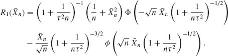
The Bayes test procedure is to reject H0 whenever R1(![]() n) ≤ R0(
n) ≤ R0(![]() n). Thus, H0 should be rejected whenever
n). Thus, H0 should be rejected whenever

But this holds if, and only if, ![]() n ≥ 0.
n ≥ 0. ![]()
Example 8.9. Let X1, X2, … be i.i.d. random variables having a normal distribution with mean μ, and variance σ2 = 1. We wish to test k = 3 composite hypotheses H-1: −∞ < μ < −1; H0: −1 ≤ μ ≤ 1; H1: μ > 1. Let μ have a prior normal distribution, μ ∼ N(0, τ2). Thus, let
![]()
and ![]() , be the prior probabilities of H−1, H0, and H1, respectively. Furthermore, let
, be the prior probabilities of H−1, H0, and H1, respectively. Furthermore, let
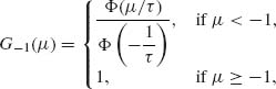
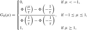
and
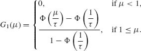
The predictive likelihood functions of the three hypotheses are then
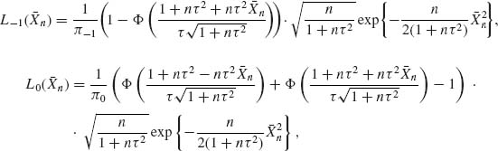
and
![]()
It follows that the posterior probabilities of Hj, j = −1, 0, 1 are as follows:
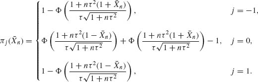
Thus, π−1(![]() n) ≥ 1 –
n) ≥ 1 – ![]() if
if
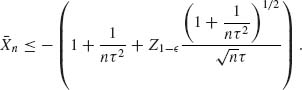
Similarly, π1(![]() n) ≥ 1 –
n) ≥ 1 – ![]() if
if
![]()
Thus, if ![]() then bn and −bn are outer stopping boundaries. In the region (−bn, bn), we have two inner boundaries (−cn, cn) such that if |
then bn and −bn are outer stopping boundaries. In the region (−bn, bn), we have two inner boundaries (−cn, cn) such that if |![]() n| < cn then H0 is accepted. The boundaries ± cn can be obtained by solving the equation
n| < cn then H0 is accepted. The boundaries ± cn can be obtained by solving the equation
![]()
cn ≥ 0 and cn > 0 only if n > n0, where 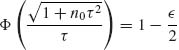 , or n0 =
 ![]() .
. ![]()
Example 8.10. Consider the problem of estimating circular probabilities in the normal case. In Example 6.4, we derived the uniformly most accurate (UMA) lower confidence limit of the function
![]()
where J is a ![]() random variable for cases of known ρ. We derive here the Bayes lower credibility limit of
random variable for cases of known ρ. We derive here the Bayes lower credibility limit of ![]() (σ2, ρ) for cases of known ρ. The minimal sufficient statistic is
(σ2, ρ) for cases of known ρ. The minimal sufficient statistic is 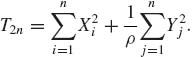 . This statistic is distributed like σ2χ2[2n] or like
 ![]() . Let ω =
. Let ω = ![]() and let ω ∼ G(τ, ν). The posterior distribution of ω, given T2n, is
and let ω ∼ G(τ, ν). The posterior distribution of ω, given T2n, is
![]()
Accordingly, if G−1(p | T2n + τ, n + ν) designates the pth quantile of this posterior distribution,
![]()
with probability one (with respect to the mixed prior distribution of T2n). Thus, we obtain that a 1–α Bayes upper credibility limit for σ2 is
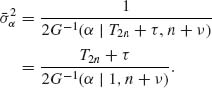
Note that if τ, and ν are close to zero then the Bayes credibility limit is very close to the non–Bayes UMA upper confidence limit derived in Example 7.4. Finally, the (1–α) Bayes lower credibility limit for ![]() (σ2, ρ) is
(σ2, ρ) is ![]() .
. ![]()
Example 8.11. We consider in the present example the problem of inverse regression. Suppose that the relationship between a controlled experimental variable x and an observed random variable Y(x) is describable by a linear regression
![]()
where ![]() is a random variable such that E{
is a random variable such that E{![]() } = 0 and E{
} = 0 and E{![]() 2} = σ2. The regression coefficients α and β are unknown. Given the results on n observations at x1, …, xn, estimate the value of ξ at which E{Y(ξ)} = η, where η is a preassigned value. We derive here Bayes confidence limits for ξ = (η –α)/β, under the assumption that m random variables are observed independently at x1 and x2, where x2 = x1 + Δ. Both x1 and Δ are determined by the design. Furthermore, we assume that the distribution of
2} = σ2. The regression coefficients α and β are unknown. Given the results on n observations at x1, …, xn, estimate the value of ξ at which E{Y(ξ)} = η, where η is a preassigned value. We derive here Bayes confidence limits for ξ = (η –α)/β, under the assumption that m random variables are observed independently at x1 and x2, where x2 = x1 + Δ. Both x1 and Δ are determined by the design. Furthermore, we assume that the distribution of ![]() is N(0, σ2) and that (α, β) has a prior bivariate normal distribution with mean (α0, β0) and covariance matrix V = (vij; i, j = 1, 2). For the sake of simplicity, we assume in the present example that σ2 is known. The results can be easily extended to the case of unknown σ2.
is N(0, σ2) and that (α, β) has a prior bivariate normal distribution with mean (α0, β0) and covariance matrix V = (vij; i, j = 1, 2). For the sake of simplicity, we assume in the present example that σ2 is known. The results can be easily extended to the case of unknown σ2.
The minimal sufficient statistic is (![]() 1,
1, ![]() 2) where
2) where ![]() i is the mean of the m observations at xi (i = 1, 2). The posterior distribution of (α, β) given (
i is the mean of the m observations at xi (i = 1, 2). The posterior distribution of (α, β) given (![]() 1,
1, ![]() 2) is the bivariate normal with mean vector
2) is the bivariate normal with mean vector
![]()
where
![]()
and I is the 2 × 2 identity matrix. Note that X is nonsingular. X is called the design matrix. The covariance matrix of the posterior distribution is
![]()
Let us denote the elements of ![]() by
by ![]() ij, i, j = 1, 2. The problem is to determine the Bayes credibility interval to the parameter ξ = (η –α)/β. Let
ij, i, j = 1, 2. The problem is to determine the Bayes credibility interval to the parameter ξ = (η –α)/β. Let ![]() and
and ![]() denote the limits of such a (1 – α) Bayes credibility interval. These limits should satisfy the posterior confidence level requirement
denote the limits of such a (1 – α) Bayes credibility interval. These limits should satisfy the posterior confidence level requirement
![]()
If we consider equal tail probabilities, these confidence limits are obtained by solving simultaneously the equations
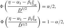
where ![]() and similarly
and similarly ![]() . By inverting, we can realize that the credibility limits
. By inverting, we can realize that the credibility limits ![]() and
and ![]() are the two roots of the quadratic equation
are the two roots of the quadratic equation
![]()
or
![]()
where
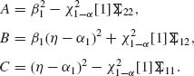
The two roots (if they exist) are
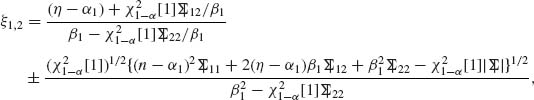
where |![]() | denotes the determinant of the posterior covariance matrix. These credibility limits exist if the discriminant
| denotes the determinant of the posterior covariance matrix. These credibility limits exist if the discriminant
![]()
is nonnegative. After some algebraic manipulations, we obtain that
![]()
where tr {·} is the trace of the matrix in {}. Thus, if m is sufficiently large, Δ* > 0 and the two credibility limits exist with probability one. ![]()
Example 8.12. Suppose that X1, …, Xn + 1 are i.i.d. random variables, having a Poisson distribution P(λ), 0 < λ < ∞. We ascribe λ a prior gamma distribution, i.e., λ ∼ G(Λ, α).
After observing X1, …, Xn, the posterior distribution of λ, given ![]() is λ | Tn ∼ G(Λ + n, Tn + α). The predictive distribution of Xn + 1, given Tn, is the negative–binomial, i.e.,
is λ | Tn ∼ G(Λ + n, Tn + α). The predictive distribution of Xn + 1, given Tn, is the negative–binomial, i.e.,
![]()
where
![]()
Let NB−1(p; ![]() , α) denote the pth quantile of NB(
, α) denote the pth quantile of NB(![]() , α). The prediction interval for Xn + 1, after observing X1, …, Xn, at level 1–α, is
, α). The prediction interval for Xn + 1, after observing X1, …, Xn, at level 1–α, is
![]()
According to Equation (2.3.12), the pth quantile of NB(![]() , α) is NB−1(p |
, α) is NB−1(p | ![]() , α) = least integer k, k ≥ 1, such that I1 –
, α) = least integer k, k ≥ 1, such that I1 – ![]() (α, k + 1) ≥ p.
(α, k + 1) ≥ p. ![]()
Example 8.13. Suppose that an n–dimensional random vector Xn has the multinormal distribution Xn | μ ∼ N(μ1n, Vn), where −∞ < μ < ∞ is unknown. The covariance matrix Vn is known. Assume that μ has a prior normal distribution, μ ∼ N(μ0, τ2). The posterior distribution of μ, given Xn, is μ | Xn ∼ N(η (Xn), Dn), where
![]()
and
![]()
Accordingly, the predictive distribution, of yet unobserved m–dimensional vector Ym | μ ∼ N(μ 1m, Vm), is
![]()
Thus, a prediction region for Ym, at level (1–α) is the ellipsoid of concentration
![]()
![]()
Example 8.14. A new drug is introduced and the physician wishes to determine a lower prediction limit with confidence probability of γ = 0.95 for the number of patients in a group of n = 10 that will be cured. If Xn is the number of patients cured among n and if θ is the individual probability to be cured the model is binomial, i.e., Xn ∼ B(n, θ). The lower prediction limit, for a given value of θ, is an integer kγ (θ) such that Pθ {Xn ≥ kγ (θ)} ≥ γ. If B−1(p;n, θ) denotes the pth quantile of the binomial B(n, θ) then kγ (θ) = max(0, B−1(1–γ ;n, θ)−1). Since the value of θ is unknown, we cannot determine kγ (θ). Lower tolerance limits, which were discussed in Section 6.5, could provide estimates to the unknown kγ (θ). A statistician may feel, however, that lower tolerance limits are too conservative, since he has good a priori information about θ. Suppose a statistician believes that θ is approximately equal to 0.8, and therefore, assigns θ a prior beta distribution β (p, q) with mean 0.8 and variance 0.01. Setting the equations for the mean and variance of a β (p, q) distribution (see Table 2.1 of Chapter 2), and solving for p and q, we obtain p = 12 and q = 3. We consider now the predictive distribution of Xn under β (12, 3) prior distribution of θ. This predictive distribution has a probability function
![]()
For n = 10, we obtain the following predictive p.d.f. pH(j) and c.d.f. fH(j). According to this predictive distribution, the probability of at least 5 cures out of 10 patients is 0.972 and for at least 6 cures is 0.925.
| j | pH(j) | FH(j) |
| 0 | 0.000034 | 0.000034 |
| 1 | 0.000337 | 0.000378 |
| 2 | 0.001790 | 0.002160 |
| 3 | 0.006681 | 0.008841 |
| 4 | 0.019488 | 0.028329 |
| 5 | 0.046770 | 0.075099 |
| 6 | 0.094654 | 0.169752 |
| 7 | 0.162263 | 0.332016 |
| 8 | 0.231225 | 0.563241 |
| 9 | 0.256917 | 0.820158 |
| 10 | 0.179842 | 1.000000 |
![]()
Example 8.15. Suppose that in a given (rather simple) inventory system (see Example 8.2) the monthly demand, X of some commodity is a random variable having a Poisson distribution P(θ), 0 < θ < ∞. We wish to derive a Bayes estimator of the expected demand θ. In many of the studies on Bayes estimator of θ, a prior gamma distribution ![]() is assumed for θ. The prior parameters τ and ν, 0 < τ, ν < ∞, are specified. Note that the prior expectation of θ is ν τ and its prior variance is ν τ2. A large prior variance is generally chosen if the prior information on θ is vague. This yields a flat prior distribution. On the other hand, if the prior information on θ is strong in the sense that we have a high prior confidence that θ lies close to a value θ0 say, pick ν τ = θ0 and ν τ2 very small, by choosing τ to be small. In any case, the posterior distribution of θ, given a sample of n i.i.d. random variables X1, …, Xn, is determined in the following manner.
is assumed for θ. The prior parameters τ and ν, 0 < τ, ν < ∞, are specified. Note that the prior expectation of θ is ν τ and its prior variance is ν τ2. A large prior variance is generally chosen if the prior information on θ is vague. This yields a flat prior distribution. On the other hand, if the prior information on θ is strong in the sense that we have a high prior confidence that θ lies close to a value θ0 say, pick ν τ = θ0 and ν τ2 very small, by choosing τ to be small. In any case, the posterior distribution of θ, given a sample of n i.i.d. random variables X1, …, Xn, is determined in the following manner. ![]() is a minimal sufficient statistic, where Tn ∼ P(nθ). The derivation of the posterior density can be based on the p.d.f. of Tn. Thus, the product of the p.d.f. of Tn by the prior p.d.f. of θ is proportional to θt + ν −1e-θ (n + 1/τ), where Tn = t. The factors that were omitted from the product of the p.d.fs are independent of θ and are, therefore, irrelevant. We recognize in the function θt + ν −1e-θ (n + 1/τ) the kernel (the factor depending on θ) of a gamma p.d.f. Accordingly, the posterior distribution of θ, given Tn, is the gamma distribution
is a minimal sufficient statistic, where Tn ∼ P(nθ). The derivation of the posterior density can be based on the p.d.f. of Tn. Thus, the product of the p.d.f. of Tn by the prior p.d.f. of θ is proportional to θt + ν −1e-θ (n + 1/τ), where Tn = t. The factors that were omitted from the product of the p.d.fs are independent of θ and are, therefore, irrelevant. We recognize in the function θt + ν −1e-θ (n + 1/τ) the kernel (the factor depending on θ) of a gamma p.d.f. Accordingly, the posterior distribution of θ, given Tn, is the gamma distribution ![]() . If we choose a squared–error loss function, then the posterior expectation is the Bayes estimator. We thus obtain the estimator
. If we choose a squared–error loss function, then the posterior expectation is the Bayes estimator. We thus obtain the estimator ![]() . Note that the unbiased and the MLE of θ is Tn/n which is not useful as long as Tn = 0, since we know that θ > 0. If certain commodities have a very slow demand (a frequently encountered phenomenon among replacement parts) then Tn may be zero even when n is moderately large. On the other hand, the Bayes estimator θ is always positive.
. Note that the unbiased and the MLE of θ is Tn/n which is not useful as long as Tn = 0, since we know that θ > 0. If certain commodities have a very slow demand (a frequently encountered phenomenon among replacement parts) then Tn may be zero even when n is moderately large. On the other hand, the Bayes estimator θ is always positive. ![]()
Example 8.16. (a) Let X1, …, XN be i.i.d. random variables having a normal distribution N(θ, 1), −∞ < θ < ∞. The minimal sufficient statistic is the sample mean ![]() . We assume that θ has a prior normal distribution N(0, τ2). We derive the Bayes estimator for the zero–one loss function,
. We assume that θ has a prior normal distribution N(0, τ2). We derive the Bayes estimator for the zero–one loss function,
![]()
The posterior distribution of θ given ![]() is normal N(
is normal N(![]() (1 + 1/nτ2)−1, (n + 1/τ2)−1). This can be verified by simple normal regression theory, recognizing that the joint distribution of (
(1 + 1/nτ2)−1, (n + 1/τ2)−1). This can be verified by simple normal regression theory, recognizing that the joint distribution of (![]() , θ) is the bivariate normal, with zero expectation and covariance matrix
, θ) is the bivariate normal, with zero expectation and covariance matrix
Thus, the posterior risk is the posterior probability of the event {|![]() − θ | ≥ δ}. This is given by
− θ | ≥ δ}. This is given by
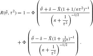
We can show then (Zacks, 1971; p. 265) that the Bayes estimator of θ is the posterior expectation, i.e.,
![]()
In this example, the minimization of the posterior variance and the maximization of the posterior probability of covering θ by the interval (![]() – δ,
– δ, ![]() + δ) is the same. This is due to the normal prior and posterior distributions.
+ δ) is the same. This is due to the normal prior and posterior distributions.
(b) Continuing with the same model, suppose that we wish to estimate the tail probability
![]()
Since the posterior distribution of θ – ξ0 given ![]() is normal, the Bayes estimator for a squared–error loss is the posterior expectation
is normal, the Bayes estimator for a squared–error loss is the posterior expectation
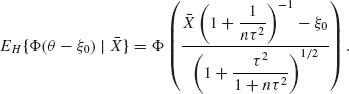
Note that this Bayes estimator is strongly consistent since, by the SLLN, ![]() → θ almost surely (a.s.), and Φ (·) is a continuous function. Hence, the Bayes estimator converges to Φ (θ – ξ0) a.s. as n → ∞. It is interesting to compare this estimator to the minimum variance unbiased estimator (MVUE) and to the MLE of the tail probability. All these estimators are very close in large samples.
→ θ almost surely (a.s.), and Φ (·) is a continuous function. Hence, the Bayes estimator converges to Φ (θ – ξ0) a.s. as n → ∞. It is interesting to compare this estimator to the minimum variance unbiased estimator (MVUE) and to the MLE of the tail probability. All these estimators are very close in large samples.
If the loss function is the absolute deviation, |![]() –
– ![]() |, rather than the squared–error, (
|, rather than the squared–error, (![]() –
–![]() )2, then the Bayes estimator of
)2, then the Bayes estimator of ![]() is the median of the posterior distribution of Φ (θ –ξ0). Since the Φ–function is strictly increasing this median is Φ (θ.5 – ξ0), where θ0.5 is the median of the posterior distribution of θ given
is the median of the posterior distribution of Φ (θ –ξ0). Since the Φ–function is strictly increasing this median is Φ (θ.5 – ξ0), where θ0.5 is the median of the posterior distribution of θ given ![]() . We thus obtain that the Bayes estimator for absolute deviation loss is
. We thus obtain that the Bayes estimator for absolute deviation loss is
This is different from the posterior expectation. ![]()
Example 8.17. In this example, we derive Bayes estimators for the parameters μ and σ2 in the normal model N(μ, σ2) for squared–error loss. We assume that X1, …, Xn, given (μ, σ2), are i.i.d. N(μ, σ2). The minimal sufficient statistic is (![]() n, Q), where
n, Q), where ![]() and
and ![]() . Let
. Let ![]() = 1/σ2 be the precision parameter, and consider the reparametrization (μ, σ2) → (μ,
= 1/σ2 be the precision parameter, and consider the reparametrization (μ, σ2) → (μ, ![]() ).
).
The likelihood function is
![]()
The following is a commonly assumed joint prior distribution for (μ, ![]() ), namely,
), namely,
![]()
and
![]()
where n0 is an integer, and 0 < ![]() < ∞. This joint prior distribution is called the Normal–Gamma prior, and denoted by
< ∞. This joint prior distribution is called the Normal–Gamma prior, and denoted by ![]() . Since
. Since ![]() n and Q are conditionally independent, given (μ,
n and Q are conditionally independent, given (μ, ![]() ), and since the distribution of Q is independent of μ, the posterior distribution of μ |
), and since the distribution of Q is independent of μ, the posterior distribution of μ | ![]() n,
n, ![]() is normal with mean
is normal with mean
![]()
and variance
![]()
![]() B is a Bayesian estimator of μ for the squared–error loss function. The posterior risk of
B is a Bayesian estimator of μ for the squared–error loss function. The posterior risk of ![]() B is
B is
![]()
The second term on the RHS is zero. Thus, the posterior risk of ![]() B is
B is
![]()
The posterior distribution of ![]() depends only on Q. Indeed, if we denote generally by p(
depends only on Q. Indeed, if we denote generally by p(![]() | μ,
| μ, ![]() ) and p(Q |
) and p(Q | ![]() ) the conditional p.d.f. of
) the conditional p.d.f. of ![]() and Q then
and Q then
![]()
Hence, the marginal posterior p.d.f. of ![]() is
is
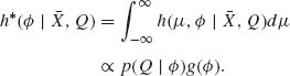
Thus, from our model, the posterior distribution of ![]() , given Q, is the gamma
, given Q, is the gamma ![]() . It follows that
. It follows that
![]()
Thus, the posterior risk of ![]() B is
B is
![]()
The Bayesian estimator of σ2 is
![]()
The posterior risk of ![]() is
is
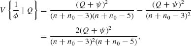
which is finite if n + n0 > 5. ![]()
Example 8.18. Consider the model of the previous example, but with priorly independent parameters μ and ![]() , i.e., we assume that h(μ,
, i.e., we assume that h(μ, ![]() ) = h(μ)g(
) = h(μ)g(![]() ), where
), where
![]()
and
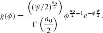
If p(![]() | μ,
| μ, ![]() ) and p(Q |
) and p(Q | ![]() ) are the p.d.f. of
) are the p.d.f. of ![]() and of Q, given μ,
and of Q, given μ, ![]() , respectively, then the joint posterior p.d.f. of (μ,
, respectively, then the joint posterior p.d.f. of (μ, ![]() ), given (
), given (![]() , Q), is
, Q), is
![]()
where A(![]() , Q) > 0 is a normalizing factor. The marginal posterior p.d.f. of μ, given (
, Q) > 0 is a normalizing factor. The marginal posterior p.d.f. of μ, given (![]() , Q), is
, Q), is
![]()
It is straightforward to show that the integral on the RHS of (8.4.18) is proportional to ![]() . Thus,
. Thus,
![]()
A simple analytic expression for the normalizing factor A* (![]() , Q) is not available. One can resort to numerical integration to obtain the Bayesian estimator of μ, namely,
, Q) is not available. One can resort to numerical integration to obtain the Bayesian estimator of μ, namely,
![]()
By the Lebesgue Dominated Convergence Theorem
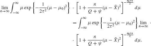
Thus, for large values of n,
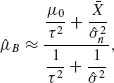
where ![]() .
.
In a similar manner, we can show that the marginal posterior p.d.f. of ![]() is
is

where B* (![]() , Q) > 0 is a normalizing factor. Note that for large values of n, g* (
, Q) > 0 is a normalizing factor. Note that for large values of n, g* (![]() |
| ![]() , Q) is approximately the p.d.f. of
, Q) is approximately the p.d.f. of ![]() .
.
In Chapter 5, we discussed the least–squares and MVUEs of the parameters in linear models. Here, we consider Bayesian estimators for linear models. Comprehensive Bayesian analysis of various linear models is given in the books of Box and Tiao (1973) and of Zellner (1971). The analysis in Zellner’s book (see Chapter III) follows a straightforward methodology of deriving the posterior distribution of the regression coefficients for informative and noninformative priors. Box and Tiao provide also geometrical representation of the posterior distributions (probability contours) and the HPD–regions of the parameters. Moreover, by analyzing the HPD–regions Box and Tiao establish the Bayesian justification to the analysis of variance and simultaneous confidence intervals of arbitrary contrasts (the Scheffé S–method). In Example 8.11, we derived the posterior distribution of the regression coefficients of the linear model Y = α + β x + ![]() , where
, where ![]() ∼ N(0, σ2) and (α, β) have a prior normal distribution. In a similar fashion the posterior distribution of β in the multiple regression model Y = Xβ +
∼ N(0, σ2) and (α, β) have a prior normal distribution. In a similar fashion the posterior distribution of β in the multiple regression model Y = Xβ + ![]() can be obtained by assuming that
can be obtained by assuming that ![]() ∼ N(0, V) and the prior distribution of β is N(β0, B). By applying the multinormal theory, we readily obtain that the posterior distribution of β, given Y, is
∼ N(0, V) and the prior distribution of β is N(β0, B). By applying the multinormal theory, we readily obtain that the posterior distribution of β, given Y, is
![]()
This result is quite general and can be applied whenever the covariance matrix V is known. Often we encounter in the literature the ![]() prior and the (observations) model
prior and the (observations) model
![]()
and
![]()
This model is more general than the previous one, since presently the covariance matrices V and B are known only up to a factor of proportionality. Otherwise, the models are equivalent. If we replace V by ![]() , where V* is a known positive definite matrix, and
, where V* is a known positive definite matrix, and ![]() , 0 <
, 0 < ![]() < ∞, is an unknown precision parameter then, by factoring V* = C* C*′, and letting Y* = (C*)−1Y, X* = (C*)−1X we obtain
< ∞, is an unknown precision parameter then, by factoring V* = C* C*′, and letting Y* = (C*)−1Y, X* = (C*)−1X we obtain
![]()
Similarly, if B = DD′ and β* = D−1β then
![]()
If X** = X* D then the previous model, in terms of Y* and X**, is reduced to
![]()
where Y* = C−1Y, X* = C−1XD, β* = D−1β, V = CC′, and B = DD′.
We obtained a linear model generalization of the results of Example 8.17. Indeed,
![]()
Thus, the Bayesian estimator of β, for the squared–error loss, ||β − ![]() ||2 is
||2 is
![]()
As in Example 8.17, the conditional predictive distribution of Y, given ![]() , is normal,
, is normal,
![]()
Hence, the marginal posterior distribution of ![]() , given Y, is the gamma distribution, i.e.,
, given Y, is the gamma distribution, i.e.,
![]()
where n is the dimension of Y. Thus, the Bayesian estimator of ![]() is
is
![]()
Finally, if ![]() = n0 then the predictive distribution of Y is the multivariate t[n0;Xβ0, I + τ2XX′], defined in (2.13.12).
= n0 then the predictive distribution of Y is the multivariate t[n0;Xβ0, I + τ2XX′], defined in (2.13.12). ![]()
Example 8.19. The following is a random growth model. We follow the model assumptions of Section 8.4.3:
![]()
where θ0, t and θ1, t vary at random according to a random–walk model, i.e.,
![]()
Thus, let θt = (θ0, t, θ1, t)′ and a′t = (1, t). The dynamic linear model is thus
![]()
Let ηt and Ct be the posterior mean and posterior covariance matrix of θt. We obtain the recursive equations
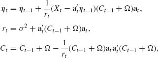
where σ2 = V{![]() t} and Ω is the covariance matrix of ωt.
t} and Ω is the covariance matrix of ωt. ![]()
Example 8.20. In order to illustrate the approximations of Section 8.5, we apply them here to a model in which the posterior p.d.f. can be computed exactly. Thus, let X1, …, Xn be conditionally i.i.d. random variables, having a common Poisson distribution P(λ), 0 < λ < ∞. Let the prior distribution of λ be that of a gamma, G(Λ, α). Thus, the posterior distribution of λ, given ![]() is like that of G(n + Λ, α + Tn), with p.d.f.
is like that of G(n + Λ, α + Tn), with p.d.f.
![]()
The MLE of λ is ![]() n = Tn/n. In this model, J(
n = Tn/n. In this model, J(![]() n) = n/
n) = n/![]() n. Thus, formula (8.5.11) yields the normal approximation
n. Thus, formula (8.5.11) yields the normal approximation
![]()
From large sample theory, we know that
![]()
Thus, the approximation to h(λ | Tn) given by
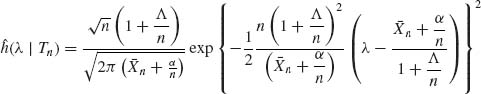
should be better than ![]() , if the sample size is not very large.
, if the sample size is not very large. ![]()
Example 8.21. We consider again the model of Example 8.20. In that model, for 0 < λ < ∞,
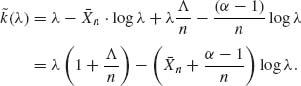
Thus,
and the maximizer of ![]() is
is
Moreover,
The normal approximation, based on ![]() n and
n and ![]() , is
, is  This is very close to the large sample approximation (8.5.15). The only difference is that α, in
 ![]() (λ | Tn), is replaced by α′ = α − 1.
(λ | Tn), is replaced by α′ = α − 1. ![]()
Example 8.22. We consider again the model of Example 8.3. In that example, Yi | λi ∼ P(λi), where λi = ![]() , i = 1, …, n. Let (X) = (X1, …, Xn)′ be the n × p matrix of covariates. The unknown parameter is β
, i = 1, …, n. Let (X) = (X1, …, Xn)′ be the n × p matrix of covariates. The unknown parameter is β ![]()
![]() (p). The prior distribution of β is normal, i.e., β ∼ N(β0, τ2I). The likelihood function is, according to Equation (8.1.8),
(p). The prior distribution of β is normal, i.e., β ∼ N(β0, τ2I). The likelihood function is, according to Equation (8.1.8),
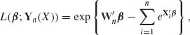
where ![]() . The prior p.d.f. is,
. The prior p.d.f. is,
![]()
Accordingly,
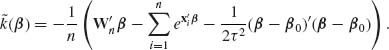
Hence,
![]()
and
![]()
The value ![]() is the root of the equation
is the root of the equation
![]()
Note that
![]()
where Δ (β) is an n × n diagonal matrix with ith diagonal element equal to eβ′Xi (i = 1, …, n). The matrix ![]() is positive definite for all β
is positive definite for all β ![]()
![]() (p). We can determine
(p). We can determine ![]() by solving the equation iteratively, starting with the LSE,
by solving the equation iteratively, starting with the LSE, ![]() , where
, where ![]() is a vector whose ith component is
is a vector whose ith component is
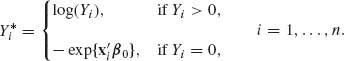
The approximating p.d.f. for h(β | (X), Yn) is the p.d.f. of the p–variate normal ![]() . This p.d.f. will be compared later numerically with a p.d.f. obtained by numerical integration and one obtained by simulation.
. This p.d.f. will be compared later numerically with a p.d.f. obtained by numerical integration and one obtained by simulation. ![]()
Example 8.23. Let (Xi, Yi), i = 1, …, n be i.i.d. random vectors, having a standard bivariate normal distribution, i.e., (X, Y)′ ∼ N![]() . The likelihood function of ρ is
. The likelihood function of ρ is
![]()
where Tn = (QX, PXY, QY) and ![]() . The Fisher information function for ρ is
. The Fisher information function for ρ is
![]()
Using the Jeffreys prior
![]()
the Bayesian estimator of ρ for the squared error loss is
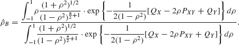
This estimator, for given values of QX, QY and PXY, can be evaluated accurately by 16–points Gaussian quadrature. For n = 16, we get from Table 2.54 of Abramowitz and Stegun (1968) the values
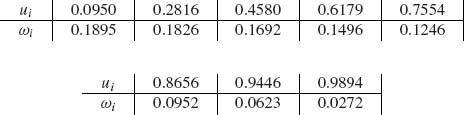
For negative values of u, we use -u; with the same weight, ωi. For a sample of size n = 10, with QX = 6.1448, QY = 16.1983, and PXY = 4.5496, we obtain ![]() B = 0.3349.
B = 0.3349. ![]()
Example 8.24. In this example, we consider evaluating the integrals in ![]() B of Example 8.23 by simulations. We simulate 100 random variables Ui ∼ R(−1, 1) i = 1, …, 100, and approximate the integrals in the numerator and denominator of
B of Example 8.23 by simulations. We simulate 100 random variables Ui ∼ R(−1, 1) i = 1, …, 100, and approximate the integrals in the numerator and denominator of ![]() θ by averages. For n = 100, and the same values of QX, QY, PXY, as in Example 8.23, we obtain the approximation
θ by averages. For n = 100, and the same values of QX, QY, PXY, as in Example 8.23, we obtain the approximation ![]() = 0.36615.
= 0.36615. ![]()
Example 8.25. We return to Example 8.22 and compute the posterior expectation of β by simulation. Note that, for a large number M of simulation runs, E{β| X, Y} is approximated by
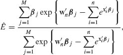
where βj is a random vector, simulated from the N(β0, τ2I) distribution.
To illustrate the result numerically, we consider a case where the observed sample contains 40 independent observations; ten for each one of the for x vectors:
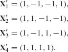
The observed values of w40 is (6, 3, 11, 29). For β′0 = (0.1, 0.1, 0.5, 0.5), we obtain the following Bayesian estimators ![]() , with M = 1000,
, with M = 1000,
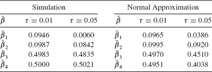
We see that when τ = 0.01 the Bayesian estimators are very close to the prior mean β0. When τ = 0.05 the Bayesian estimators might be quite different than β0. In Example 8.22, we approximated the posterior distribution of β by a normal distribution. For the values in this example the normal approximation yields similar results to those of the simulation. ![]()
Example 8.26. Consider the following repetitive problem. In a certain manufacturing process, a lot of N items is produced every day. Let Mj, j = 1, 2, …, denote the number of defective items in the lot of the jth day. The parameters M1, M2, … are unknown. At the end of each day, a random sample of size n is selected without replacement from that day’s lot for inspection. Let Xj denote the number of defectives observed in the sample of the jth day. The distribution of Xj is the hypergeometric H(N, Mj, n), j = 1, 2, …. Samples from different days are (conditionally) independent (given M1, M2, …). In this problem, it is often reasonable to assume that the parameters M1, M2, … are independent random variables having the same binomial distribution B(N, θ). θ is the probability of defectives in the production process. It is assumed that θ does not change in time. The value of θ is, however, unknown. It is simple to verify that for a prior B(N, θ) distribution of M, and a squared–error loss function, the Bayes estimator of Mj is
![]()
The corresponding Bayes risk is
![]()
A sequence of empirical Bayes estimators is obtained by substituting in ![]() j a consistent estimator of θ based on the results of the first (j − 1) days. Under the above assumption on the prior distribution of M1, M2, …, the predictive distribution of X1, X2, … is the binomial B(n, θ). A priori, for a given value of θ, X1, X2, … can be considered as i.i.d. random variables having the mixed distribution B(n, θ). Thus,
j a consistent estimator of θ based on the results of the first (j − 1) days. Under the above assumption on the prior distribution of M1, M2, …, the predictive distribution of X1, X2, … is the binomial B(n, θ). A priori, for a given value of θ, X1, X2, … can be considered as i.i.d. random variables having the mixed distribution B(n, θ). Thus, ![]() j−1 =
j−1 = 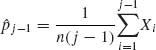 , for j ≥ 2, is a sequence of consistent estimators of θ. The corresponding sequence of empirical Bayes estimators is
![]()
The posterior risk of ![]() j given (Xj,
j given (Xj, ![]() j − 1) is
j − 1) is
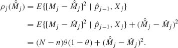
We consider now the conditional expectation of ρj(![]() j) given Xj. This is given by
j) given Xj. This is given by
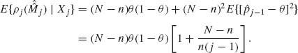
Notice that this converges as j → ∞ to ρ (θ). ![]()
Example 8.27. This example shows the application of empirical Bayes techniques to the simultaneous estimation of many probability vectors. The problem was motivated by a problem of assessing the readiness probabilities of military units based on exercises of big units. For details, see Brier, Zacks, and Marlow (1986).
A large number, N, of units are tested independently on tasks that are classified into K categories. Each unit obtains on each task the value 1 if it is executed satisfactorily and the value 0 otherwise. Let i, i = 1, …, N be the index of the ith unit, and j, j = 1, …, k the index of a category. Unit i was tested on Mij tasks of category j. Let Xij denote the number of tasks in category j on which the ith unit received a satisfactory score. Let θij denote the probability of the ith unit executing satisfactorily a task of category j. There are N parametric vectors θi = (θi1, …, θiK)′, i = 1, …, N, to be estimated.
The model is that, conditional on θi, Xi1, …, XiK are independent random variables, having binomial distributions, i.e.,
![]()
In addition, the vectors θi (i = 1, …, N) are i.i.d. random variables, having a common distribution. Since Mij were generally large, but not the same, we have used first the variance stabilizing transformation
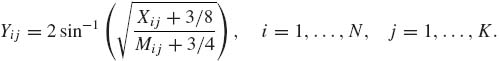
For large values of Mij the asymptotic distribution of Yij is N(ηij, 1/Mij), where ηij = 2sin−1![]() , as shown in Section 7.6.
, as shown in Section 7.6.
Let Yi = (Yi1, …, YiK)′, i = 1, …, N. The parametric empirical Bayes model is that (Yi, θi) are i.i.d, i = 1, …, N,
![]()
and
![]()
where ηi = (ηi1, …, ηiK)′ and
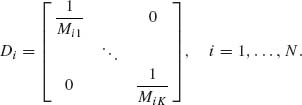
The prior parameters μ and ![]() are unknown. Note that if μ and
are unknown. Note that if μ and ![]() are given then η, η2, …, ηN are a posteriori independent, given Y1, …, YN. Furthermore, the posterior distribution of ηi, given Yi, is
are given then η, η2, …, ηN are a posteriori independent, given Y1, …, YN. Furthermore, the posterior distribution of ηi, given Yi, is
![]()
where
![]()
Thus, if μ and ![]() are given, the Bayesian estimator of ηi, for a squared–error loss function L(ηi,
are given, the Bayesian estimator of ηi, for a squared–error loss function L(ηi, ![]() i) = ||
i) = ||![]() i – ηi||2, is the posterior mean, i.e.,
i – ηi||2, is the posterior mean, i.e.,
![]()
The empirical Bayes method estimates μ and ![]() from all the data. We derive now MLEs of μ and
from all the data. We derive now MLEs of μ and ![]() . These MLEs are then substituted in
. These MLEs are then substituted in ![]() i(μ,
i(μ, ![]() ) to yield empirical Bayes estimators of ηi.
) to yield empirical Bayes estimators of ηi.
Note that Yi | μ, ![]() ∼ N(μ,
∼ N(μ, ![]() + Di), i = 1, …, N. Hence, the log–likelihood function of (μ,
+ Di), i = 1, …, N. Hence, the log–likelihood function of (μ, ![]() ), given the data (Y1, …, YN), is
), given the data (Y1, …, YN), is
![]()
The vector ![]() (
(![]() ), which maximizes l(μ,
), which maximizes l(μ, ![]() ), for a given
), for a given ![]() is
is
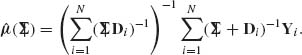
Substituting ![]() (
(![]() ) in l(μ,
) in l(μ, ![]() ) and finding
) and finding ![]() that maximizes the expression can yield the MLE
that maximizes the expression can yield the MLE ![]() . Another approach, to find the MLE, is given by the E–M algorithm. The E–M algorithm considers the unknown parameters η1, …, ηN as missing data. The algorithm is an iterative process, having two phases in each iteration. The first phase is the E–phase, in which the conditional expectation of the likelihood function is determined, given the data and the current values of (μ,
. Another approach, to find the MLE, is given by the E–M algorithm. The E–M algorithm considers the unknown parameters η1, …, ηN as missing data. The algorithm is an iterative process, having two phases in each iteration. The first phase is the E–phase, in which the conditional expectation of the likelihood function is determined, given the data and the current values of (μ, ![]() ). In the next phase, the M–phase, the conditionally expected likelihood is maximized by determining the maximizing arguments
). In the next phase, the M–phase, the conditionally expected likelihood is maximized by determining the maximizing arguments ![]() . More specifically, let
. More specifically, let
![]()
be the log–likelihood of (μ, ![]() ) if η1, …, ηN were known. Let (μ(p),
) if η1, …, ηN were known. Let (μ(p), ![]() (p)) be the estimator of (μ,
(p)) be the estimator of (μ, ![]() ) after p iterations, p ≥ 0, where μ(0),
) after p iterations, p ≥ 0, where μ(0), ![]() (0) are initial estimates.
(0) are initial estimates.
In the (p + 1)st iteration, we start (the E–phase) by determining
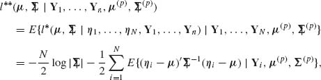
where the conditional expectation is determined as though μ(p) and ![]() (p) are the true values. It is well known that if E{X} = ξ and the covariance matrix of X is
(p) are the true values. It is well known that if E{X} = ξ and the covariance matrix of X is ![]() (X) then E{X′AX} = μ′Aμ + tr{AC(X)}, where tr {·} is the trace of the matrix (see, Seber, 1977, p. 13). Thus,
(X) then E{X′AX} = μ′Aμ + tr{AC(X)}, where tr {·} is the trace of the matrix (see, Seber, 1977, p. 13). Thus,
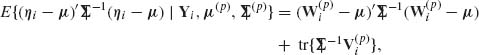
where, ![]() , in which
, in which ![]() , and
, and ![]() , i = 1, …, N. Thus,
, i = 1, …, N. Thus,
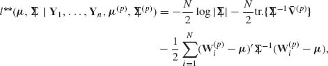
where ![]() . In phase– M, we determine μ(p + 1) and
. In phase– M, we determine μ(p + 1) and ![]() (p + 1) by maximizing l** (μ,
(p + 1) by maximizing l** (μ, ![]() | …).
| …).
One can immediately verify that
![]()
Moreover,
![]()
where ![]() , and
, and
![]()
Finally, the matrix maximizing l** is
![]()
We can prove recursively, by induction on p, that
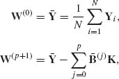
where ![]() and
and
![]()
Thus,
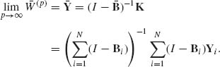
One continues iterating until μ(p) and ![]() (p) do not change significantly.
(p) do not change significantly.
Brier, Zacks, and Marlow (1986) studied the efficiency of these empirical Bayes estimators, in comparison to the simple MLE, and to another type of estimator that will be discussed in Chapter 9. ![]()