CHAPTER 9
Advanced Topics in Estimation Theory
PART I: THEORY
In the previous chapters, we discussed various classes of estimators, which attain certain optimality criteria, like minimum variance unbiased estimators (MVUE), asymptotic optimality of maximum likelihood estimators (MLEs), minimum mean–squared–error (MSE) equivariant estimators, Bayesian estimators, etc. In this chapter, we present additional criteria of optimality derived from the general statistical decision theory. We start with the game theoretic criterion of minimaxity and present some results on minimax estimators. We then proceed to discuss minimum risk equivariant and standard estimators. We discuss the notion of admissibility and present some results of Stein on the inadmissibility of some classical estimators. These examples lead to the so–called Stein–type and Shrinkage estimators.
9.1 MINIMAX ESTIMATORS
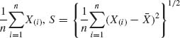
Given a class ![]() of estimators, the risk function associated with each d
of estimators, the risk function associated with each d ![]()
![]() is R(d, θ), θ
is R(d, θ), θ ![]() Θ. The maximal risk associated with d is R*(d) =
Θ. The maximal risk associated with d is R*(d) = ![]() R(d, θ). If in
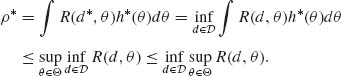
R(d, θ). If in ![]() there is an estimator d* that minimizes R*(d) then d* is called a minimax estimator. That is,
there is an estimator d* that minimizes R*(d) then d* is called a minimax estimator. That is,
![]()
A minimax estimator may not exist in ![]() . We start with some simple results.
. We start with some simple results.
Lemma 9.1.1. Let ![]() = {F(x;θ), θ
= {F(x;θ), θ ![]() Θ} be a family of distribution functions and
Θ} be a family of distribution functions and ![]() a class of estimators of θ. Suppose that d*
a class of estimators of θ. Suppose that d* ![]()
![]() and d* is a Bayes estimator relative to some prior distribution H* (θ) and that the risk function R*(d, θ) does not depend on θ. Then d* is a minimax estimator.
and d* is a Bayes estimator relative to some prior distribution H* (θ) and that the risk function R*(d, θ) does not depend on θ. Then d* is a minimax estimator.
Proof. Since R(d*, θ) = ρ* for all θ in Θ, and d* is Bayes against H*(θ) we have
On the other hand, since ρ* = R(d*, θ) for all θ
From (9.1.1) and (9.1.2), we obtain that
(9.1.3) ![]()
This means that d* is minimax. QED
Lemma 9.1.1 can be generalized by proving that if there exists a sequence of Bayes estimators with prior risks converging to ρ*, where ρ* is a constant risk of d*, then d* is minimax. We obtain this result as a corollary of the following lemma.
Lemma 9.1.2. Let {Hk;k ≥ 1} be a sequence of prior distributions on Θ and let {![]() k;k ≥ 1} be the corresponding sequence of Bayes estimators with prior risks ρ (
k;k ≥ 1} be the corresponding sequence of Bayes estimators with prior risks ρ (![]() k, Hk). If there exists an estimator d* for which
k, Hk). If there exists an estimator d* for which
then d* is minimax.
Proof. If d* is not a minimax estimator, there exists an estimator ![]() such that
such that
Moreover, for each k ≥ 1 since ![]() k is Bayes,
k is Bayes,
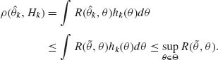
But (9.1.5) in conjunction with (9.1.6) contradict (9.1.4). Hence, d* is minimax. QED
9.2 MINIMUM RISK EQUIVARIANT, BAYES EQUIVARIANT, AND STRUCTURAL ESTIMATORS
In Section 5.7.1, we discussed the structure of models that admit equivariant estimators with respect to certain groups of transformations. In this section, we return to this subject and investigate minimum risk, Bayes and minimax equivariant estimators. The statistical model under consideration is specified by a sample space ![]() and a family of distribution functions
and a family of distribution functions ![]() = {F(x;θ);θ
= {F(x;θ);θ ![]() Θ}. Let
Θ}. Let ![]() be a group of transformations that preserves the structure of the model, i.e., g
be a group of transformations that preserves the structure of the model, i.e., g![]() =
= ![]() for all g
for all g ![]()
![]() , and the induced group
, and the induced group ![]() of transformations on Θ has the property that
of transformations on Θ has the property that ![]() Θ = Θ for all
Θ = Θ for all ![]()
![]()
![]() . An equivariant estimator
. An equivariant estimator ![]() (X) of θ was defined as one which satisfies the structural property that
(X) of θ was defined as one which satisfies the structural property that ![]() (gX) =
(gX) = ![]()
![]() (X) for all g
(X) for all g ![]()
![]() .
.
In cases of various orbits of ![]() in Θ, we may index the orbits by a parameter, say ω (θ). The risk function of an equivariant estimator
in Θ, we may index the orbits by a parameter, say ω (θ). The risk function of an equivariant estimator ![]() (X) is then R(
(X) is then R(![]() , ω (θ)). Bayes equivariant estimators can be considered. These are equivariant estimators that minimize the prior risk associated with θ, relative to a prior distribution H(θ). We assume that ω (θ) is a function of θ for which the following prior risk exists, namely,
, ω (θ)). Bayes equivariant estimators can be considered. These are equivariant estimators that minimize the prior risk associated with θ, relative to a prior distribution H(θ). We assume that ω (θ) is a function of θ for which the following prior risk exists, namely,
(9.2.1) 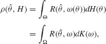
where K(ω) is the prior distribution of ω (θ), induced by H(θ). Let U(X) be a maximal invariant statistic with respect to ![]() . Its distribution depends on θ only through ω (θ). Suppose that g(u;ω) is the probability density function (p.d.f.) of U(X) under ω. Let k(ω | U) be the posterior p.d.f. of ω given U(X). The prior risk of θ can be written then as
. Its distribution depends on θ only through ω (θ). Suppose that g(u;ω) is the probability density function (p.d.f.) of U(X) under ω. Let k(ω | U) be the posterior p.d.f. of ω given U(X). The prior risk of θ can be written then as
(9.2.2) ![]()
where Eω|U{R(![]() , ω)} is the posterior risk of θ, given U(X). An equivariant estimator
, ω)} is the posterior risk of θ, given U(X). An equivariant estimator ![]() K is Bayes against K(ω) if it minimizes Eω|U{R(
K is Bayes against K(ω) if it minimizes Eω|U{R(![]() , ω)}.
, ω)}.
As discussed earlier, the Bayes equivariant estimators are relevant only if there are different orbits of ![]() in Θ. Another approach to the estimation problem, if there are no minimum risk equivariant estimators, is to derive formally the Bayes estimators with respect to invariant prior measures (like the Jeffreys improper priors). Such an approach to the above problem of estimating variance components was employed by Tiao and Tan (1965) and by Portnoy (1971). We discuss now formal Bayes estimators more carefully.
in Θ. Another approach to the estimation problem, if there are no minimum risk equivariant estimators, is to derive formally the Bayes estimators with respect to invariant prior measures (like the Jeffreys improper priors). Such an approach to the above problem of estimating variance components was employed by Tiao and Tan (1965) and by Portnoy (1971). We discuss now formal Bayes estimators more carefully.
9.2.1 Formal Bayes Estimators for Invariant Priors
Formal Bayes estimators with respect to invariant priors are estimators that minimize the expected risk, when the prior distribution used is improper. In this section, we are concerned with invariant prior measures, such as the Jeffreys noninformative prior h(θ)dθ ∝|I(θ)|1/2dθ. With such improper priors, the minimum risk estimators can often be formally derived as in Section 5.7. The resulting estimators are called formal Bayes estimators. For example, if ![]() = {F(x;θ); −∞ < θ < ∞} is a family of location parameters distributions (of the translation type), i.e., the p.d.f.s are f(x;θ) =
= {F(x;θ); −∞ < θ < ∞} is a family of location parameters distributions (of the translation type), i.e., the p.d.f.s are f(x;θ) = ![]() (x− θ) then, for the group
(x− θ) then, for the group ![]() of real translations, the Jeffreys invariant prior is h(θ)dθ ∝ dθ. If the loss function is L(
of real translations, the Jeffreys invariant prior is h(θ)dθ ∝ dθ. If the loss function is L(![]() , θ) = (
, θ) = (![]() – θ)2, the formal Bayes estimator is
– θ)2, the formal Bayes estimator is
(9.2.3) 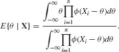
Making the transformation Y = X(1) – θ, where X(1) ≤ … ≤ X(n), we obtain
(9.2.4) 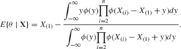
This is the Pitman estimator (5.7.10).
When ![]() is a family of location and scale parameters, with p.d.f.s
is a family of location and scale parameters, with p.d.f.s
(9.2.5) ![]()
we consider the group ![]() of real affine transformations
of real affine transformations ![]() = {[α, β]; −∞ < α < ∞, 0 < β < ∞}. The fisher information matrix of (μ, σ) for
= {[α, β]; −∞ < α < ∞, 0 < β < ∞}. The fisher information matrix of (μ, σ) for ![]() is, if exists,
is, if exists,
(9.2.6) ![]()
where
(9.2.7) ![]()
(9.2.8) ![]()
and
(9.2.9) ![]()
Accordingly, |I(μ, σ)| ![]() and the Jeffreys invariant prior is
and the Jeffreys invariant prior is
(9.2.10) ![]()
If the invariant loss function for estimating μ is L(![]() , μ, σ) =
, μ, σ) = ![]() then the formal Bayes estimator of μ is
then the formal Bayes estimator of μ is
(9.2.11) 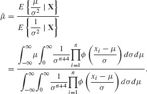
Let y1 ≤ … ≤ yn represent realization of the order statistics X(1) ≤ … ≤ X(n). Consider the change of variables
(9.2.12) 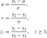
then the formal Bayes estimator of μ is
For estimating σ, we consider the invariant loss function L(![]() , σ) = (
, σ) = (![]() –σ)2/σ2. The formal Bayes estimator is then
–σ)2/σ2. The formal Bayes estimator is then
Note that the formal Bayes estimator (9.2.13) is equivalent to the Pitman estimator, for a location parameter family (with known scale parameter). The estimator (9.2.14) is the Pitman estimator for a scale parameter family.
Formal Bayes estimation can be used also when the model has parameters that are invariant with respect to the group of transformations ![]() . In the variance components model discussed in Example 9.3, the variance ratio ρ = τ2/σ2 is such an invariant parameter. These parameters are called also nuisance parameters for the transformation model.
. In the variance components model discussed in Example 9.3, the variance ratio ρ = τ2/σ2 is such an invariant parameter. These parameters are called also nuisance parameters for the transformation model.
9.2.2 Equivariant Estimators Based on Structural Distributions
Fraser (1968) introduced structural distributions of parameters in cases of invariance structures, when all the parameters of the model can be transformed by the transformations in ![]() . Fraser’s approach does not require the assignment of a prior distribution to the unknown parameters. This approach is based on changing the variables of integration from those representing the observable random variables to those representing the parameters. We start the explanation by considering real parameter families. More specifically, let
. Fraser’s approach does not require the assignment of a prior distribution to the unknown parameters. This approach is based on changing the variables of integration from those representing the observable random variables to those representing the parameters. We start the explanation by considering real parameter families. More specifically, let ![]() = {F(x;θ);θ
= {F(x;θ);θ ![]() Θ} be a family of distributions, where Θ is an interval on the real line. Let
Θ} be a family of distributions, where Θ is an interval on the real line. Let ![]() be a group of one–to–one transformations, preserving the structure of the model. For the simplicity of the presentation, we assume that the distribution functions of
be a group of one–to–one transformations, preserving the structure of the model. For the simplicity of the presentation, we assume that the distribution functions of ![]() are absolutely continuous and the transformation in
are absolutely continuous and the transformation in ![]() can be represented as functions over
can be represented as functions over ![]() × Θ. Choose in Θ a standard or reference point e and let U be a random variable, having the distribution F(u;e), which is the standard distribution. Let
× Θ. Choose in Θ a standard or reference point e and let U be a random variable, having the distribution F(u;e), which is the standard distribution. Let ![]() (u) be the p.d.f. of the standard distribution. The structural model assumes that if a random variable X has a distribution function F(x;θ); when θ =
(u) be the p.d.f. of the standard distribution. The structural model assumes that if a random variable X has a distribution function F(x;θ); when θ = ![]() e, g
e, g ![]()
![]() , then X = gU. Thus, the structural model can be expressed in the formula
, then X = gU. Thus, the structural model can be expressed in the formula
(9.2.15) ![]()
Assume that G(u, θ) is differentiable with respect to u and θ. Furthermore, let
(9.2.16) ![]()
The function G(u, θ) satisfies the equivariance condition that
![]()
with an invariant inverse; i.e.,
![]()
We consider now the variation of u as a function of θ for a fixed value of x. Writing the probability element of U at u in the form
(9.2.17) ![]()
we obtain for every fixed x a distribution function for θ, over Θ, with p.d.f.
where m(θ, x) = ![]() . The distribution function corresponding to k(θ, x) is called the structural distribution of θ given X = x. Let L(
. The distribution function corresponding to k(θ, x) is called the structural distribution of θ given X = x. Let L(![]() (x), θ) be an invariant loss function. The structural risk of
(x), θ) be an invariant loss function. The structural risk of ![]() (x) is the expectation
(x) is the expectation
(9.2.19) ![]()
An estimator θ0(x) is called minimum risk structural estimator if it minimizes R(![]() (x)). The p.d.f. (9.2.18) corresponds to one observation on X. Suppose that a sample of n independent identically distributed (i.i.d.) random variables X1, …, Xn is represented by the point x = (x1, …, xn). As before, θ is a real parameter. Let V(X) be a maximal invariant statistic with respect to
(x)). The p.d.f. (9.2.18) corresponds to one observation on X. Suppose that a sample of n independent identically distributed (i.i.d.) random variables X1, …, Xn is represented by the point x = (x1, …, xn). As before, θ is a real parameter. Let V(X) be a maximal invariant statistic with respect to ![]() . The distribution of V(X) is independent of θ. (We assume that Θ has one orbit of
. The distribution of V(X) is independent of θ. (We assume that Θ has one orbit of ![]() .) Let k(v) be the joint p.d.f. of the maximal invariant V(X). Let u1 = G−1 (x1, θ) and let
.) Let k(v) be the joint p.d.f. of the maximal invariant V(X). Let u1 = G−1 (x1, θ) and let ![]() (u| x) be the conditional p.d.f. of the standard variable U = [θ]−1X, given V = v. This conditional p.d.f. of θ, for a given x is then, like in (9.2.18),
(u| x) be the conditional p.d.f. of the standard variable U = [θ]−1X, given V = v. This conditional p.d.f. of θ, for a given x is then, like in (9.2.18),
(9.2.20) ![]()
If the model depends on a vector θ of parameters we make the appropriate generalizations as will be illustrated in Example 9.4.
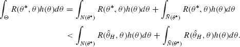
We conclude the present section with some comment concerning minimum properties of formal Bayes and structural estimators. Girshick and Savage (1951) proved that if all equivariant estimators in the location parameter model have finite risk, then the Pitman estimator (9.2.24) is minimax. Generally, if a formal Bayes estimator with respect to an invariant prior measure (as the Jeffreys priors) and invariant loss function is an equivariant estimator, and if the parameter space Θ has only one orbit of ![]() , then the risk function of the formal Bayes estimator is constant over Θ. Moreover, if this formal Bayes estimator can be obtained as a limit of a sequence of proper Bayes estimators, or if there exists a sequence of proper Bayes estimators and the lower limit of their prior risks is not smaller than the risk of the formal Bayes estimator, then the formal Bayes is a minimax estimator. Several theorems are available concerning the minimax nature of the minimum risk equivariant estimators. The most famous is the Hunt–Stein Theorem (Zacks, 1971; p. 346).
, then the risk function of the formal Bayes estimator is constant over Θ. Moreover, if this formal Bayes estimator can be obtained as a limit of a sequence of proper Bayes estimators, or if there exists a sequence of proper Bayes estimators and the lower limit of their prior risks is not smaller than the risk of the formal Bayes estimator, then the formal Bayes is a minimax estimator. Several theorems are available concerning the minimax nature of the minimum risk equivariant estimators. The most famous is the Hunt–Stein Theorem (Zacks, 1971; p. 346).
9.3 THE ADMISSIBILITY OF ESTIMATORS
9.3.1 Some Basic Results
The class of all estimators can be classified according to the given risk function into two subclasses: admissible and inadmissible ones.
Definition. An estimator ![]() 1(x) is called inadmissible with respect to a risk function R(
1(x) is called inadmissible with respect to a risk function R(![]() , θ) if there exists another estimator
, θ) if there exists another estimator ![]() 2(x) for which
2(x) for which
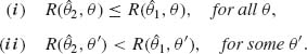
From the decision theoretic point of view inadmissible estimators are inferior. It is often not an easy matter to prove that a certain estimator is admissible. On the other hand, several examples exist of the inadmissibility of some commonly used estimators. A few examples will be provided later in this section. We start, however, with a simple and important lemma.
Lemma 9.3.1 (Blyth, 1951). If the risk function R(![]() , θ) is continuous in θ for each
, θ) is continuous in θ for each ![]() , and if the prior distribution H(θ) has a positive p.d.f. at all θ then the Bayes estimator
, and if the prior distribution H(θ) has a positive p.d.f. at all θ then the Bayes estimator ![]() H(x) is admissible.
H(x) is admissible.
Proof. By negation, if ![]() H(x) is inadmissible then there exists another estimator
H(x) is inadmissible then there exists another estimator ![]() * (x) for which (9.3.1) holds. Let θ* be a point at which the strong inequality (ii) of (9.3.1) holds. Since R(
* (x) for which (9.3.1) holds. Let θ* be a point at which the strong inequality (ii) of (9.3.1) holds. Since R(![]() , θ) is continuous in θ for each
, θ) is continuous in θ for each ![]() , there exists a neighborhood N(θ*) around θ* over which the inequality (ii) holds for all θ
, there exists a neighborhood N(θ*) around θ* over which the inequality (ii) holds for all θ ![]() N(θ*). Since h(θ) > 0 for all θ, PH{N(θ*)} > 0. Finally from inequality (i) we obtain that
N(θ*). Since h(θ) > 0 for all θ, PH{N(θ*)} > 0. Finally from inequality (i) we obtain that
The left–hand side of (9.3.2) is the prior risk of θ* and the right–hand side is the prior risk of ![]() H. But this result contradicts the assumption that
H. But this result contradicts the assumption that ![]() H is Bayes with respect to H(θ). QED
H is Bayes with respect to H(θ). QED
All the examples, given in Chapter 8, of proper Bayes estimators illustrate admissible estimators. Improper Bayes estimators are not necessarily admissible. For example, in the N(μ, σ2) case, when both parameters are unknown, the formal Bayes estimator of σ2 with respect to the Jeffreys improper prior h(σ2) dσ2 ∝ dσ2/σ2 is Q/(n – 3), where Q = Σ(Xi – ![]() )2. This estimator is, however, inadmissible, since Q/(n + 1) has a smaller MSE for all σ2. There are also admissible estimators that are not Bayes. For example, the sample mean
)2. This estimator is, however, inadmissible, since Q/(n + 1) has a smaller MSE for all σ2. There are also admissible estimators that are not Bayes. For example, the sample mean ![]() from a normal distribution N(θ, 1) is an admissible estimator with respect to a squared–error loss. However,
from a normal distribution N(θ, 1) is an admissible estimator with respect to a squared–error loss. However, ![]() is not a proper Bayes estimator. It is a limit (as k → ∞) of the Bayes estimators derived in Section 8.4,
is not a proper Bayes estimator. It is a limit (as k → ∞) of the Bayes estimators derived in Section 8.4, ![]() k =
k = ![]() is also an improper Bayes estimator with respect to the Jeffreys improper prior h(θ)dθ ∝ dθ. Indeed, for such an improper prior
is also an improper Bayes estimator with respect to the Jeffreys improper prior h(θ)dθ ∝ dθ. Indeed, for such an improper prior
(9.3.3) 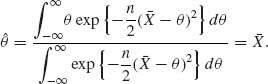
The previous lemma cannot establish the admissibility of the sample mean ![]() . We provide here several lemmas that can be used.
. We provide here several lemmas that can be used.
Lemma 9.3.2. Assume that the MSE of an estimator ![]() 1 attains the Cramér–Rao lower bound (under the proper regularity conditions) for all θ, −∞ < θ < ∞, which is
1 attains the Cramér–Rao lower bound (under the proper regularity conditions) for all θ, −∞ < θ < ∞, which is
(9.3.4) ![]()
where B1(θ) is the bias of ![]() 1. Moreover, if for any estimator
1. Moreover, if for any estimator ![]() 2 having a Cramér–Rao lower bound C2(θ), the inequality C2(θ) ≤ C1(θ) for all θ implies that B2(θ) = B1(θ) for all θ, then θ1 is admissible.
2 having a Cramér–Rao lower bound C2(θ), the inequality C2(θ) ≤ C1(θ) for all θ implies that B2(θ) = B1(θ) for all θ, then θ1 is admissible.
Proof. If ![]() 1 is inadmissible, there exists an estimator
1 is inadmissible, there exists an estimator ![]() 2 such that
2 such that
![]()
with a strict inequality at some θ′. Since R(![]() 1, θ) = C1(θ) for all θ, we have
1, θ) = C1(θ) for all θ, we have
for all θ. But, according to the hypothesis, (9.3.5) implies that B1(θ) = B2(θ) for all θ. Hence, C1(θ) = C2(θ) for all θ. But this contradicts the assumption that R(![]() 2, θ′) < R(
2, θ′) < R(![]() 1, θ′). Hence,
1, θ′). Hence, ![]() 1 is admissible. QED
1 is admissible. QED
Lemma 9.3.2 can be applied to prove that, in the case of a sample from N(0, σ2), ![]() is an admissible estimator of σ2. (The MVUE and the MLE are inadmissible!) In such an application, we have to show that the hypotheses of Lemma 9.3.2 are satisfied. In the N(0, σ2) case, it requires lengthy and tedious computations (Zacks, 1971, p. 373). Lemma 9.3.2 is also useful to prove the following lemma (Girshick and Savage, 1951).
is an admissible estimator of σ2. (The MVUE and the MLE are inadmissible!) In such an application, we have to show that the hypotheses of Lemma 9.3.2 are satisfied. In the N(0, σ2) case, it requires lengthy and tedious computations (Zacks, 1971, p. 373). Lemma 9.3.2 is also useful to prove the following lemma (Girshick and Savage, 1951).
Lemma 9.3.3. Let X be a one–parameter exponential type random variable, with p.d.f.
![]()
–∞ < ![]() < ∞. Then
< ∞. Then ![]() = X is an admissible estimator of its expectation μ (
= X is an admissible estimator of its expectation μ (![]() ) = + K′(
) = + K′(![]() ), for the quadratic loss function (
), for the quadratic loss function (![]() –μ)2/σ2(
–μ)2/σ2(![]() ); where σ2(
); where σ2(![]() ) = + K″(
) = + K″(![]() ) is the variance of X.
) is the variance of X.
Proof. The proof of the present lemma is based on the following points. First X is an unbiased estimator of μ (![]() ). Since the distribution of X is of the exponential type, its variance σ2(
). Since the distribution of X is of the exponential type, its variance σ2(![]() ) is equal to the Cramér–Rao lower bound, i.e.,
) is equal to the Cramér–Rao lower bound, i.e.,
(9.3.6) 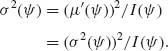
This implies that I(![]() ) = σ2(
) = σ2(![]() ), which can be also derived directly. If
), which can be also derived directly. If ![]() (X) is any other estimator of μ(
(X) is any other estimator of μ(![]() ) satisfying the Cramér–Rao regularity condition with variance D2(
) satisfying the Cramér–Rao regularity condition with variance D2(![]() ), such that
), such that
(9.3.7) ![]()
then from the Cramér–Rao inequality
(9.3.8) ![]()
where B(![]() ) is the bias function of
) is the bias function of ![]() (X). Thus, we arrived at the inequality
(X). Thus, we arrived at the inequality
(9.3.9) ![]()
all −∞ < ![]() < ∞. This implies that
< ∞. This implies that
for all −∞ < ![]() < ∞. From (9.3.10), we obtain that either B(
< ∞. From (9.3.10), we obtain that either B(![]() ) = 0 for all
) = 0 for all ![]() or
or
(9.3.11) ![]()
for all ![]() such that B(
such that B(![]() ) ≠ 0. Since B(
) ≠ 0. Since B(![]() ) is a decreasing function, either B(
) is a decreasing function, either B(![]() ) = 0 for all
) = 0 for all ![]() ≥
≥ ![]() 0 or B(
0 or B(![]() ) ≠ 0 for all
) ≠ 0 for all ![]() ≥
≥ ![]() 0. Let G(
0. Let G(![]() ) be a function defined so that G(
) be a function defined so that G(![]() 0) = 1/B(
0) = 1/B(![]() 0) and G′(
0) and G′(![]() ) = 1/2 for all
) = 1/2 for all ![]() ≥
≥ ![]() 0; i.e.,
0; i.e.,
(9.3.12) ![]()
Since 1/B(![]() ) is an increasing function and
) is an increasing function and ![]() , it is always above G(
, it is always above G(![]() ) on
) on ![]() ≥
≥ ![]() 0. It follows that
0. It follows that
(9.3.13) ![]()
In a similar manner, we can show that ![]() or
or ![]() . This implies that B(
. This implies that B(![]() ) = 0 for all
) = 0 for all ![]() . Finally, since the bias function of
. Finally, since the bias function of ![]() (X) = X is also identically zero we obtain from the previous lemma that
(X) = X is also identically zero we obtain from the previous lemma that ![]() (X) is admissible. QED
(X) is admissible. QED
Karlin (1958) established sufficient condition for the admissibility of a linear estimator
of the expected value of T in the one parameter exponential family, with p.d.f.
![]()
Theorem 9.3.1 (Karlin) Let X have a one–parameter exponential distribution, with ![]() . Sufficient conditions for the admissibility of (9.3.14) as estimator of Eθ {T(X)}, under squared–error loss, is
. Sufficient conditions for the admissibility of (9.3.14) as estimator of Eθ {T(X)}, under squared–error loss, is
![]()
or
![]()
where ![]() .
.
For a proof of this theorem, see Lehmann and Casella (1998, p. 331).
Considerable amount of research was conducted on the question of the admissibility of formal or generalized Bayes estimators. Some of the important results will be discussed later. We address ourselves here to the question of the admissibility of equivariant estimators of the location parameter in the one–dimensional case. We have seen that the minimum risk equivariant estimator of a location parameter θ, when finite risk equivariant estimators exist, is the Pitman estimator
![]()
The question is whether this estimator is admissible. Let Y = (X(2) – X(1), …, X(n) – X(1)) denote the maximal invariant statistic and let f(x | y) the conditional distribution of X(1), when θ = 0, given Y = y. Stein (1959) proved the following.
Theorem 9.3.2. If ![]() (X) is the Pitman estimator and
(X) is the Pitman estimator and
then ![]() (X) is an admissible estimator of θ with respect to the squared–error loss.
(X) is an admissible estimator of θ with respect to the squared–error loss.
We omit the proof of this theorem, which can be found in Stein’s paper (1959) or in Zacks (1971, pp. 388–393). The admissibility of the Pitman estimator of a two–dimensional location parameter was proven later by James and Stein (1960). The Pitman estimator is not admissible, however, if the location parameter is a vector of order p ≥ 3. This result, first established by Stein (1956) and by James and Stein (1960), will be discussed in the next section.
The Pitman estimator is a formal Bayes estimator. It is admissible in the real parameter case. The question is under what conditions formal Bayes estimators in general are admissible. Zidek (1970) established sufficient conditions for the admissibility of formal Bayes estimators having a bounded risk.
9.3.2 The Inadmissibility of Some Commonly Used Estimators
In this section, we discuss a few well–known examples of some MLE or best equivariant estimators that are inadmissible. The first example was developed by Stein (1956) and James and Stein (1960) established the inadmissibility of the MLE of the normal mean vector θ, in the N(θ, I) model, when the dimension of θ is p ≥ 3. The loss function considered is the squared–error loss, ![]() . This example opened a whole area of research and led to the development of a new type of estimator of a location vector, called the Stein estimators. Another example that will be presented establishes the inadmissibility of the best equivariant estimator of the variance of a normal distribution when the mean is unknown. This result is also due to Stein (1964). Other related results will be mentioned too.
. This example opened a whole area of research and led to the development of a new type of estimator of a location vector, called the Stein estimators. Another example that will be presented establishes the inadmissibility of the best equivariant estimator of the variance of a normal distribution when the mean is unknown. This result is also due to Stein (1964). Other related results will be mentioned too.
I. The Inadmissibility of the MLE in the N(θ, I) Case, With p ≥ 3
Let X be a random vector of p components, with p ≥ 3. Furthermore assume that X∼ N(θ}, I). The assumption that the covariance matrix of X is I, is not a restrictive one, since if X ∼ N(θ, V), with a known V, we can consider the case of Y = C−1X, where V = CC′. Obviously, Y ∼ N(η}, I) where η = C−1θ. Without loss of generality, we also assume that the sample size is n = 1. The MLE of θ is X itself. Consider the squared–error loss function ![]() . Since X is unbiased, the risk of the MLE is R* = p for all θ. We show now an estimator that has a risk function smaller than p for all θ, and when θ is close to zero its risk is close to 2. The estimator suggested by Stein is
. Since X is unbiased, the risk of the MLE is R* = p for all θ. We show now an estimator that has a risk function smaller than p for all θ, and when θ is close to zero its risk is close to 2. The estimator suggested by Stein is
This estimator is called the James–Stein estimator. The risk function of (9.3.16) is
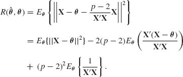
The first term on the RHS of (9.3.17) is p. We notice that X′X ∼ χ2![]() . Accordingly,
. Accordingly,
where ![]() . We turn now to the second term on the RHS of (9.3.17). Let
. We turn now to the second term on the RHS of (9.3.17). Let ![]() and
and ![]() . Note that U ∼ N(||θ||, 1) is independent of V and V ∼ χ2[p – 1]. Indeed, we can write
. Note that U ∼ N(||θ||, 1) is independent of V and V ∼ χ2[p – 1]. Indeed, we can write
(9.3.19) ![]()
where A = (I – θθ′/||θ||2) is an idempotent matrix of rank p – 1. Hence, V∼ χ2[p – 1]. Moreover, Aθ/||θ|| = 0. Hence, U and V are independent. Furthermore,
(9.3.20) 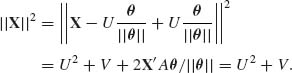
We let W = ||X||2, and derive the p.d.f. of U/W. This is needed, since the second term on the RHS of (9.3.17) is -2(p – 2)[1 – ||θ||Eθ{U/W}]. Since U and V are independent, their joint p.d.f. is
(9.3.21) 
Thus, the joint p.d.f. of U and W is
(9.3.22) 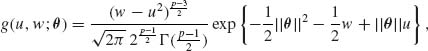
0 ≤ u2 ≤ w ≤ ∞. The p.d.f. of R = U/W is then
(9.3.23) ![]()
Accordingly,
(9.3.24) 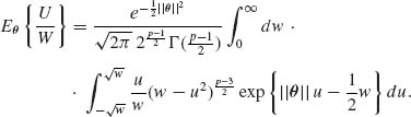
By making the change of variables to t = ![]() and expanding
and expanding ![]() we obtain, after some manipulations,
we obtain, after some manipulations,
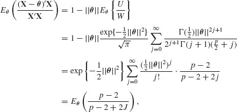
where ![]() . From (9.3.17), (9.3.18) and (9.3.25), we obtain
. From (9.3.17), (9.3.18) and (9.3.25), we obtain
(9.3.26) ![]()
Note that when θ = 0, P0[J = 0] = 1 and R(θ, 0) = 2. On the other hand, ![]() . The estimator
. The estimator ![]() given by (9.3.17) has smaller risk than the MLE for all θ values. In the above development, there is nothing to tell us whether (9.3.17) is itself admissible. Note that (9.3.17) is not an equivariant estimator with respect to the group of real affine transformations, but it is equivariant with respect to the group of orthogonal transformations (rotations). If the vector X has a known covariance matrix V, the estimator (9.3.17) should be modified to
given by (9.3.17) has smaller risk than the MLE for all θ values. In the above development, there is nothing to tell us whether (9.3.17) is itself admissible. Note that (9.3.17) is not an equivariant estimator with respect to the group of real affine transformations, but it is equivariant with respect to the group of orthogonal transformations (rotations). If the vector X has a known covariance matrix V, the estimator (9.3.17) should be modified to
(9.3.27) ![]()
This estimator is equivariant with respect to the group ![]() of nonsingular transformations X → AX. Indeed, the covariance matrix of Y = AX is
of nonsingular transformations X → AX. Indeed, the covariance matrix of Y = AX is ![]() = AVA′. Therefore, Y′
= AVA′. Therefore, Y′![]() ,−1Y = X′V−1X for every A
,−1Y = X′V−1X for every A ![]()
![]() .
.
Baranchick (1973) showed, in a manner similar to the above, that in the usual multiple regression model with normal distributions the commonly used MLEs of the regression coefficients are inadmissible. More specifically, let X1, …, Xn be a sample of n i.i.d. (p + 1) dimensional random vectors, having a multinormal distribution N(θ, ![]() ). Consider the regression of Y = X1 on Z = (X2, …, Xp + 1)′. If we consider the partition θ′ = (η, ζ′) and
). Consider the regression of Y = X1 on Z = (X2, …, Xp + 1)′. If we consider the partition θ′ = (η, ζ′) and
![]()
then the regression of Y on Z is given by
![]()
where α = η – β′ζ and β = V−1C. The problem is to estimate the vector of regression coefficients β. The least–squares estimators (LSE) is 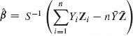 , where
 ![]() . Y1, …, Yn and Z1, …, Zn are the sample statistics corresponding to X1, …, Xn.
. Y1, …, Yn and Z1, …, Zn are the sample statistics corresponding to X1, …, Xn.
Consider the loss function
(9.3.28) ![]()
With respect to this loss function Baranchick proved that the estimators
(9.3.29) 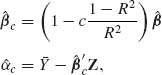
have risk functions smaller than that of the LSEs (MLEs) ![]() and
and ![]() , at all the parameter values, provided
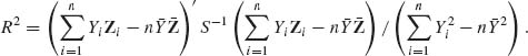
, at all the parameter values, provided ![]() and p ≥ 3,n ≥ p + 2. R2 is the squared–multiple correlation coefficient given by
and p ≥ 3,n ≥ p + 2. R2 is the squared–multiple correlation coefficient given by
The proof is very technical and is omitted. The above results of Stein and Baranchick on the inadmissibility of the MLEs can be obtained from the following theorem of Cohen (1966) that characterizes all the admissible linear estimate of the mean vector of multinormal distributions. The theorem provides only the conditions for the admissibility of the estimators, and contrary to the results of Stein and Baranchick, it does not construct alternative estimators.
Theorem 9.3.3 (Cohen, 1966). Let X∼ N(θ, I) where the dimension of X is p. Let ![]() = AX be an estimator of θ, where A is a p × p matrix of known coefficients. Then
= AX be an estimator of θ, where A is a p × p matrix of known coefficients. Then ![]() is admissible with respect to the squared–error loss ||
is admissible with respect to the squared–error loss ||![]() – θ||2 if and only if A is symmetric and its eigenvalues α i (i = 1, …, p) satisfy the inequality.
– θ||2 if and only if A is symmetric and its eigenvalues α i (i = 1, …, p) satisfy the inequality.
(9.3.30) ![]()
with equality to 1 for at most two of the eigenvalues.
For a proof of the theorem, see Cohen (1966) or Zacks (1971, pp. 406–408). Note that for the MLE of θ the matrix A is I, and all the eigenvalues are equal to 1. Thus, if p ≥ 3, X is an inadmissible estimator. If we shrink the MLE towards the origin and consider the estimator θλ = λ X with 0 < λ < 1 then the resulting estimator is admissible for any dimension p. Indeed, ![]() λ is actually the Bayes estimator (8.4.31) with A1 = V = I,
λ is actually the Bayes estimator (8.4.31) with A1 = V = I, ![]() , = τ2I and A2 = 0. In this case, the Bayes estimator is
, = τ2I and A2 = 0. In this case, the Bayes estimator is ![]() , where 0 < τ < ∞. We set λ = τ2/(1 + τ2). According to Lemma 9.3.1, this proper Bayes estimator is admissible. In Section 9.3.3, we will discuss more meaningful adjustment of the MLE to obtain admissible estimators of θ.
, where 0 < τ < ∞. We set λ = τ2/(1 + τ2). According to Lemma 9.3.1, this proper Bayes estimator is admissible. In Section 9.3.3, we will discuss more meaningful adjustment of the MLE to obtain admissible estimators of θ.
II. The Inadmissibility of the Best Equivariant Estimators of the Scale Parameter When the Location Parameter is Unknown
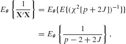
Consider first the problem of estimating the variance of a normal distribution N(μ, σ2) when the mean μ is unknown. Let X1, …, Xn be i.i.d. random variables having such distribution. Let (![]() , Q) be the minimal sufficient statistic,
, Q) be the minimal sufficient statistic, ![]() and
and ![]() . We have seen that the minimum risk equivariant estimator, with respect to the quadratic loss
. We have seen that the minimum risk equivariant estimator, with respect to the quadratic loss ![]() . Stein (1964) showed that this estimator is, however, inadmissible! The estimator
. Stein (1964) showed that this estimator is, however, inadmissible! The estimator
has uniformly smaller risk function. We present here Stein’s proof of this inadmissibility.
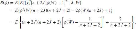
Let S = Q + n![]() 2. Obviously, S ∼ χ2[n;nμ2/2σ2] ∼ χ2[n + 2J] where J ∼ P(nμ2/2σ2). Consider the scale equivariant estimators that are functions of (Q, S). Their structure is f(Q, S) =
2. Obviously, S ∼ χ2[n;nμ2/2σ2] ∼ χ2[n + 2J] where J ∼ P(nμ2/2σ2). Consider the scale equivariant estimators that are functions of (Q, S). Their structure is f(Q, S) = ![]() . Moreover, the conditional distribution of Q/S given J is the beta distribution
. Moreover, the conditional distribution of Q/S given J is the beta distribution ![]() . Furthermore given J, Q/S and S are conditionally independent. Note that for
. Furthermore given J, Q/S and S are conditionally independent. Note that for ![]() we use the function
we use the function ![]() . Consider the estimator
. Consider the estimator
(9.3.32) 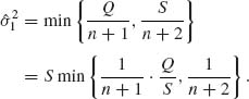
Here, 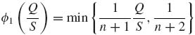 . The risk function, for the quadratic loss L(
![]() , σ2) = (
, σ2) = (![]() 2–σ2)2/σ4 is, for any function
2–σ2)2/σ4 is, for any function ![]() ,
,
(9.3.33) 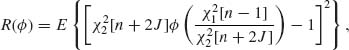
where ![]() and
and ![]() . Let W = Q/S. Then,
. Let W = Q/S. Then,
We can also write,
We notice that ![]() 1(W) ≤
1(W) ≤ ![]() 0(W). Moreover, if
0(W). Moreover, if ![]() then
then ![]() 1(W) =
1(W) = ![]() 0(W), and the first and third terms on the RHS of (9.3.35) are zero. Otherwise,
0(W), and the first and third terms on the RHS of (9.3.35) are zero. Otherwise,
![]()
Hence,
for all J and W, with strict inequality on a (J, W) set having positive probability. From (9.3.34) and (9.3.36) we obtain that R(![]() 1) < R(
1) < R(![]() 0). This proves that
0). This proves that ![]() is inadmissible.
is inadmissible.
The above method of Stein can be used to prove the inadmissibility of equivariant estimators of the variance parameters also in other normal models. See for example, Klotz, Milton and Zacks (1969) for a proof of the inadmissibility of equivariant estimators of the variance components in Model II of ANOVA.
Brown (1968) studied the question of the admissibility of the minimum risk (best) equivariant estimators of the scale parameter σ in the general location and scale parameter model, with p.d.f.s f(x;μ, σ) = ![]() . The loss functions considered are invariant bowl–shaped functions, L(δ). These are functions that are nonincreasing for δ ≤ δ0 and nondecreasing for δ > δ0 for some δ0. Given the order statistic X(1) ≤ … ≤ X(n) of the sample, let
. The loss functions considered are invariant bowl–shaped functions, L(δ). These are functions that are nonincreasing for δ ≤ δ0 and nondecreasing for δ > δ0 for some δ0. Given the order statistic X(1) ≤ … ≤ X(n) of the sample, let ![]() =
=  and Zi = (X(i) –
 ![]() )/S, i = 3, …, n. Z = (Z3, …, Zn)′ is a maximal invariant with respect to the group
)/S, i = 3, …, n. Z = (Z3, …, Zn)′ is a maximal invariant with respect to the group ![]() of real affine transformations. The best equivariant estimator of ω = σk is of the form
of real affine transformations. The best equivariant estimator of ω = σk is of the form ![]() 0 =
0 = ![]() 0(Z)Sk, where
0(Z)Sk, where ![]() 0(Z) is an optimally chosen function. Brown proved that the estimator
0(Z) is an optimally chosen function. Brown proved that the estimator
(9.3.37) 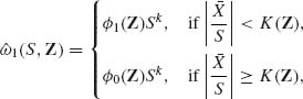
where K(Z) is appropriately chosen functions, and ![]() 1(Z) <
1(Z) < ![]() 0(Z) has uniformly smaller risk than
0(Z) has uniformly smaller risk than ![]() 0. This established the inadmissibility of the best equivariant estimator, when the location parameter is unknown, for general families of distributions and loss functions. Arnold (1970) provided a similar result in the special case of the family of shifted exponential distributions, i.e., f(x;μ, σ) = I{x ≥
0. This established the inadmissibility of the best equivariant estimator, when the location parameter is unknown, for general families of distributions and loss functions. Arnold (1970) provided a similar result in the special case of the family of shifted exponential distributions, i.e., f(x;μ, σ) = I{x ≥ ![]() .
.
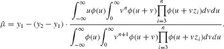
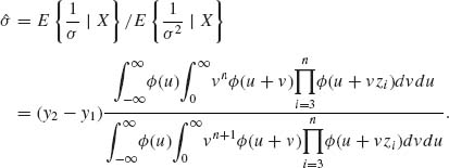
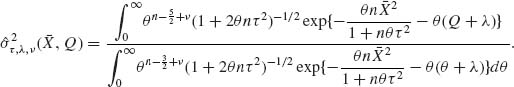
Brewster and Zidek (1974) showed that in certain cases one can refine Brown’s approach by constructing a sequence of improving estimators converging to a generalized Bayes estimator. The risk function of this estimator does not exceed that of the best equivariant estimators. In the normal case N(μ, σ2), this estimator is of the form ![]() (Z)Q, where
(Z)Q, where
with ![]() . The conditional expectations in (9.3.38) are computed with μ = 0 and σ = 1. Brewster and Zidek (1974) provided a general group theoretic framework for deriving such estimators in the general case.
. The conditional expectations in (9.3.38) are computed with μ = 0 and σ = 1. Brewster and Zidek (1974) provided a general group theoretic framework for deriving such estimators in the general case.
9.3.3 Minimax and Admissible Estimators of the Location Parameter
In Section 9.3.1, we presented the James–Stein proof that the MLE of the location parameter vector in the N(θ, I) case with dimension p ≥ 3 is inadmissible. It was shown that the estimator (9.3.17) is uniformly better than the MLE. The estimator (9.3.17) is, however, also inadmissible. Several studies have been published on the question of adjusting estimator (9.3.17) to obtain minimax estimators. In particular, see Berger and Bock (1976). Baranchick (1970) showed that a family of minimax estimators of θ is given by
where S = X′X and ![]() (S) is a function satisfying the conditions:
(S) is a function satisfying the conditions:
(9.3.40) ![]()
If the model is N(θ, σ2I) with known σ2 then the above result holds with S = X′X/σ2. If σ2 is unknown and ![]() 2 is an estimator of σ2 having a distribution like σ2· χ2[ν]/(ν + 2) then we substitute in (9.3.39) S = X′X/
2 is an estimator of σ2 having a distribution like σ2· χ2[ν]/(ν + 2) then we substitute in (9.3.39) S = X′X/![]() 2. The minimaxity of (9.3.39) is established by proving that its risk function, for the squared–error loss, does not exceed the constant risk, R* = p, of the MLE X. Note that the MLE, X, is also minimax. In addition, (9.3.39) can be improved by
2. The minimaxity of (9.3.39) is established by proving that its risk function, for the squared–error loss, does not exceed the constant risk, R* = p, of the MLE X. Note that the MLE, X, is also minimax. In addition, (9.3.39) can be improved by
(9.3.41) 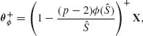
where a+ = max(a, 0). These estimators are not necessarily admissible. Admissible and minimax estimators of θ similar to (9.3.39) were derived by Strawderman (1972) for cases of known σ2 and p ≥ 5. These estimators are
(9.3.42) ![]()
where ![]() for p = 5 and 0 ≤ a ≤ 1 for p ≥ 6, also
for p = 5 and 0 ≤ a ≤ 1 for p ≥ 6, also
![]()
in which G(x;ν) = P{G(1, ν) ≤ x}. In Example 9.9, we show that θa(X) are generalized Bayes estimators for the squared–error loss and the hyper–prior model
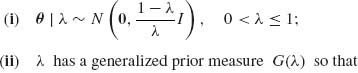
![]()
Note that if a < 1 then G(λ) is a proper prior and ![]() (X) is a proper Bayes estimator. For a proof of the admissibility for the more general case of
(X) is a proper Bayes estimator. For a proof of the admissibility for the more general case of ![]() see Lin (1974).
see Lin (1974).
9.3.4 The Relationship of Empirical Bayes and Stein–Type Estimators of the Location Parameter in the Normal Case
Efron and Morris (1972a, 1972b, 1973) show the connection between the estimator (9.3.16) and empirical Bayes estimation of the mean vector of a multinormal distribution. Ghosh (1992) present a comprehensive comparison of Empirical Bayes and the Stein–type estimators, in the case where X ∼ N(θ, I). See also the studies of Lindley and Smith (1972), Casella (1985), and Morris (1983).
Recall that in parametric empirical Bayes procedures, one estimates the unknown prior parameters, from a model of the predictive distribution of X, and substitutes the estimators in the formulae of the Bayesian estimators. On the other hand, in hierarchical Bayesian procedures one assigns specific hyper prior distributions for the unknown parameters of the prior distributions. The two approaches may sometimes result with similar estimators.
Starting with the simple model of p–variate normal X| θ ∼ N(θ, I), and θ ∼ N(0, τ2I), the Bayes estimator of θ, for the squared–error loss L(![]() , θ) = ||
, θ) = ||![]() – θ||2, is
– θ||2, is ![]() B = (1 – B)X, where B = 1/(1 + τ2). The predictive distribution of X is N(0, B−1I). Thus, the predictive distribution of X′X is like that of B−1χ2[p]. Thus, for p > 3, (p – 2)/X′X is predictive–unbiased estimator of B. Substituting this estimator for B in
B = (1 – B)X, where B = 1/(1 + τ2). The predictive distribution of X is N(0, B−1I). Thus, the predictive distribution of X′X is like that of B−1χ2[p]. Thus, for p > 3, (p – 2)/X′X is predictive–unbiased estimator of B. Substituting this estimator for B in ![]() B yields the parametric empirical Bayes estimator
B yields the parametric empirical Bayes estimator
(9.3.44) ![]()
![]() EB derived here is identical with the James–Stein estimator (9.3.16). If we change the Bayesian model so that θ ∼ N(μ 1, I), with μ known, then the Bayesian estimator is
EB derived here is identical with the James–Stein estimator (9.3.16). If we change the Bayesian model so that θ ∼ N(μ 1, I), with μ known, then the Bayesian estimator is ![]() B = (1 – B)X + Bμ 1, and the corresponding empirical Bayes estimator is
B = (1 – B)X + Bμ 1, and the corresponding empirical Bayes estimator is
(9.3.45) 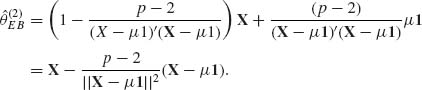
If both μ and τ are unknown, the resulting empirical Bayes estimator is
(9.3.46) 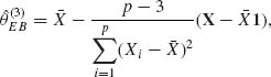
where ![]() .
.
Ghosh (1992) showed that the predictive risk function of ![]() , namely, the trace of the MSE matrix
, namely, the trace of the MSE matrix ![]() is
is
(9.3.47) ![]()
Thus, ![]() has smaller predictive risk than the MLE
has smaller predictive risk than the MLE ![]() ML = X if p ≥ 4.
ML = X if p ≥ 4.
The Stein–type estimator of the parametric vector β in the linear model X ∼ Aβ + ![]() is
is
(9.3.48) ![]()
where ![]() is the LSE and
is the LSE and
(9.3.49) ![]()
It is interesting to compare this estimator of β with the ridge regression estimator (5.4.3), in which we substitute for the optimal k value the estimator pσ2/![]() ′
′![]() . The ridge regression estimators obtains the form
. The ridge regression estimators obtains the form
(9.3.50) ![]()
There is some analogy but the estimators are obviously different. A comprehensive study of the property of the Stein–type estimators for various linear models is presented in the book of Judge and Bock (1978).
PART II: EXAMPLES
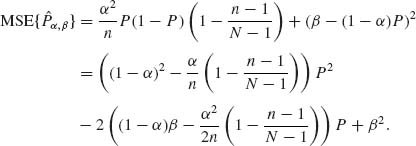
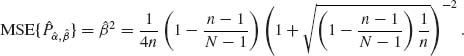
Example 9.1. Let X be a binomial B(n, θ) random variable. n is known, 0 < θ < 1. If we let θ have a prior beta distribution, i.e., θ ∼ β (ν1, ν2) then the posterior distribution of θ given X is the beta distribution β (ν1 +X, ν2 + n – X). Consider the linear estimator ![]() . The MSE of
. The MSE of ![]() α, β is
α, β is
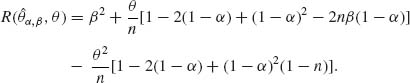
We can choose α0 and β0 so that R(![]() α0, β0, θ) = (β0)2. For this purpose, we set the equations
α0, β0, θ) = (β0)2. For this purpose, we set the equations
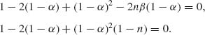
The two roots are
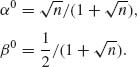
With these constants, we obtain the estimator
![]()
with constant risk
![]()
We show now that θ* is a minimax estimator of θ for a squared–error loss by specifying a prior beta distribution for which θ* is Bayes.
The Bayes estimator for the prior β (ν1, ν2) is
![]()
In particular, if ![]() then
then ![]() . This proves that θ is minimax.
. This proves that θ is minimax.
Finally, we compare the MSE of this minimax estimator with the variance of the MVUE, X/n, which is also an MLE. The variance of ![]() = X/n is θ (1 – θ)/n. V{
= X/n is θ (1 – θ)/n. V{![]() } at θ = 1/2 assumes its maximal value of 1/4n. This value is larger than R(θ*, θ). Thus, we know that around θ = 1/2 the minimax estimator has a smaller MSE than the MVUE. Actually, by solving the quadratic equation
} at θ = 1/2 assumes its maximal value of 1/4n. This value is larger than R(θ*, θ). Thus, we know that around θ = 1/2 the minimax estimator has a smaller MSE than the MVUE. Actually, by solving the quadratic equation
![]()
we obtain the two limits of the interval around θ = 1/2 over which the minimax estimator is better. These limits are given by
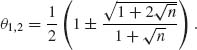
![]()
Example 9.2.
![]()
But ρ (![]() k, k) → n−1 as k→ ∞. This proves that
k, k) → n−1 as k→ ∞. This proves that ![]() is minimax.
is minimax.
Example 9.3. Consider the problem of estimating the variance components in the Model II of analysis of variance. We have k blocks of n observations on the random variables, which are represented by the linear model
![]()
where eij are i.i.d. N(0, σ2); a1, …, ak are i.i.d. random variables distributed like N(0, τ2), independently of {eij}. In Example 3.3, we have established that a minimal sufficient statistic is 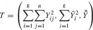 . This minimal sufficient statistic can be represented by
 ![]() , where
, where
and
![]()
ρ = τ2/σ2 is the variance ratio, ![]() = 1, 2, 3 are three independent chi–squared random variables. Consider the group
= 1, 2, 3 are three independent chi–squared random variables. Consider the group ![]() of real affine transformations,
of real affine transformations, ![]() = {[α, β]; −∞ < α < ∞, 0 < β < ∞}, and the quadratic loss function L(
= {[α, β]; −∞ < α < ∞, 0 < β < ∞}, and the quadratic loss function L(![]() , θ) = (
, θ) = (![]() – θ)2/θ2. We notice that all the parameter points (μ, σ2, τ2) such that τ2/σ2 = ρ belong to the same orbit. The values of ρ, 0 < ρ < ∞, index the various possible orbits in the parameter space. The maximal invariant reduction of T* is
– θ)2/θ2. We notice that all the parameter points (μ, σ2, τ2) such that τ2/σ2 = ρ belong to the same orbit. The values of ρ, 0 < ρ < ∞, index the various possible orbits in the parameter space. The maximal invariant reduction of T* is
![]()
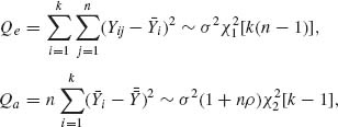
Thus, every equivariant estimator of σ2 is the form
![]()
where U = Qa/Qe, ![]() (U) and f(U) are chosen functions. Note that the distribution of U depends only on ρ. Indeed,
(U) and f(U) are chosen functions. Note that the distribution of U depends only on ρ. Indeed, ![]() . The risk function of an equivariant estimator
. The risk function of an equivariant estimator ![]() is (Zacks, 1970)
is (Zacks, 1970)

If K(ρ) is any prior distribution of the variance ratio ρ, the prior risk EK{R(f, ρ)} is minimized by choosing f(U) to minimize the posterior expectation given U, i.e.,
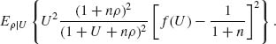
The function fK(U) that minimizes this posterior expectation is
![]()
The Bayes equivariant estimator of σ2 is obtained by substituting fK(u) in ![]() . For more specific results, see Zacks (1970b).
. For more specific results, see Zacks (1970b). ![]()
Example 9.4. Let X1, …, Xn be i.i.d. random variables having a location and scale parameter exponential distribution, i.e.,
![]()
–∞ < μ < ∞, 0 < σ < ∞.
A minimal sufficient statistic is (X(1), Sn), where X(1) ≤ … ≤ X(n) and Sn = ![]() . We can derive the structural distribution on the basis of the minimal sufficient statistic. Recall that X(1) and Sn are independent and
. We can derive the structural distribution on the basis of the minimal sufficient statistic. Recall that X(1) and Sn are independent and
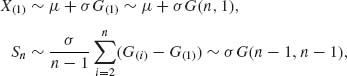
where G(1) ≤ … ≤ G(n) is an order statistic from a standard exponential distribution G(1, 1), corresponding to μ = 0, σ = 1.
The group of transformation under consideration is ![]() = {[a, b]; −∞ < a, −∞ < a < ∞, 0 < b < ∞}. The standard point is the vector (G(1), SG), where G(1) = (X(1)–μ)/σ and SG = Sn/σ. The Jacobian of this transformation is J(X(1), Sn, μ, σ) =
= {[a, b]; −∞ < a, −∞ < a < ∞, 0 < b < ∞}. The standard point is the vector (G(1), SG), where G(1) = (X(1)–μ)/σ and SG = Sn/σ. The Jacobian of this transformation is J(X(1), Sn, μ, σ) = ![]() . Moreover, the p.d.f. of (G(1), SG) is
. Moreover, the p.d.f. of (G(1), SG) is
![]()
Hence, the structural distribution of (μ, σ) given (X(1), Sn) has the p.d.f.
![]()
for −∞ < μ ≤ X(1), 0 < σ < ∞.
The minimum risk structural estimators in the present example are obtained in the following manner. Let L(![]() , μ, σ) = (
, μ, σ) = (![]() – μ)2/σ2 be the loss function for estimating μ. Then the minimum risk estimator is the μ–expectation. This is given by
– μ)2/σ2 be the loss function for estimating μ. Then the minimum risk estimator is the μ–expectation. This is given by
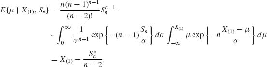
where ![]() .
.
It is interesting to notice that while the MLE of μ is X(1), the minimum risk structural estimator might be considerably smaller, but close to the Pitman estimator.
The minimum risk structural estimator of σ, for the loss function L(![]() , σ) = (
, σ) = (![]() –σ)2/σ2, is given by
–σ)2/σ2, is given by
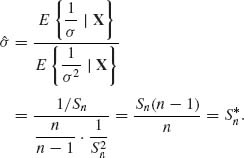
One can show that ![]() is also the minimum risk equivariant estimator of σ.
is also the minimum risk equivariant estimator of σ. ![]()
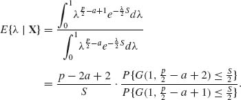
Example 9.5. A minimax estimator might be inadmissible. We show such a case in the present example. Let X1, …, Xn be i.i.d. random variables having a normal distribution, like N(μ, σ2), where both μ and σ2 are unknown. The objective is to estimate σ2 with the quadratic loss L(![]() 2, σ2) = (
2, σ2) = (![]() 2–σ2)2/σ4. The best equivariant estimator with respect to the group
2–σ2)2/σ4. The best equivariant estimator with respect to the group ![]() of real affine transformation is
of real affine transformation is ![]() , where
, where ![]() . This estimator has a constant risk
. This estimator has a constant risk ![]() . Thus,
. Thus, ![]() is minimax. However,
is minimax. However, ![]() 2 is dominated uniformly by the estimator (9.3.31) and is thus inadmissible.
2 is dominated uniformly by the estimator (9.3.31) and is thus inadmissible. ![]()
Example 9.6. In continuation of Example 9.5, given the minimal sufficient statistics (![]() n, Q), the Bayes estimator of σ2, with respect to the squared error loss, and the prior assumption that μ and σ2 are independent, μ ∼ N(0, τ2) and 1/2σ2∼ G(λ, ν), is
n, Q), the Bayes estimator of σ2, with respect to the squared error loss, and the prior assumption that μ and σ2 are independent, μ ∼ N(0, τ2) and 1/2σ2∼ G(λ, ν), is
This estimator is admissible since h(μ, σ2) > 0 for all (μ, σ2) and the risk function is continuous in (μ, σ2). ![]()
Example 9.7. Let X1, …, Xn be i.i.d. random variables, having the location parameter exponential density f(x;μ) = e−(x – μ)I{x ≥ μ}. The minimal sufficient statistic is ![]() . Moreover, X(1)∼ μ + G(n, 1). Thus, the UMVU estimator of μ is
. Moreover, X(1)∼ μ + G(n, 1). Thus, the UMVU estimator of μ is ![]() . According to (9.3.15), this estimator is admissible. Indeed, by Basu’s Theorem, the invariant statistic Y = (X(2) – X(1), X(3) – X(2), …, X(n) – X(n – 1)) is independent of X(1). Thus
. According to (9.3.15), this estimator is admissible. Indeed, by Basu’s Theorem, the invariant statistic Y = (X(2) – X(1), X(3) – X(2), …, X(n) – X(n – 1)) is independent of X(1). Thus
![]()
and
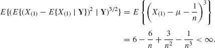
![]()
Example 9.8. Let Y ∼ N(θ, I), where θ = Hβ,
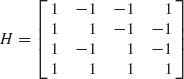
and β′ = (β1, β2, β3, β4). Note that ![]() is an orthogonal matrix. The LSE of β is
is an orthogonal matrix. The LSE of β is ![]() , and the LSE of θ is
, and the LSE of θ is ![]() = H(H′H)−1H′ = Y. The eigenvalues of H(H′H)−1H′ are αi = 1, for i = 1, …, 4. Thus, according to Theorem 9.3.3,
= H(H′H)−1H′ = Y. The eigenvalues of H(H′H)−1H′ are αi = 1, for i = 1, …, 4. Thus, according to Theorem 9.3.3, ![]() is admissible.
is admissible. ![]()
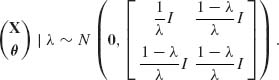
Example 9.9. Let X ∼ N(θ, I). X is a p–dimensional vector. We derive the generalized Bayes estimators of θ, for squared–error loss, and the Bayesian hyper–prior (9.3.43). This hyper–prior is
![]()
and
![]()
The joint distribution of (X′, θ′)′, given λ, is
Hence, the conditional distribution of θ, given (X, λ) is
![]()
The marginal distribution of X, given λ, is ![]() . Thus, the density of the posterior distribution of λ, given X, is
. Thus, the density of the posterior distribution of λ, given X, is
![]()
where S = X′X. It follows that the generalized Bayes estimator of θ, given X is
![]()
where
![]()
PART III: PROBLEMS
Section 9.1
9.1.1 Consider a finite population of N units. M units have the value x = 1 and the rest have the value x = 0. A random sample of size n is drawn without replacement. Let X be the number of sample units having the value x = 1. The conditional distribution of X, given M, n is H(N, M, n). Consider the problem of estimating the parameter P = M/N, with a squared–error loss. Show that the linear estimator ![]() , with
, with 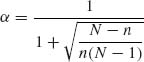 and
and ![]() has a constant risk.
has a constant risk.
9.1.2 Let ![]() be a family of prior distributions on Θ. The Bayes risk of H
be a family of prior distributions on Θ. The Bayes risk of H ![]()
![]() is ρ(H) = ρ (
is ρ(H) = ρ (![]() H, H), where
H, H), where ![]() H is a Bayesian estimator of θ, with respect to H. H* is called least–favorable in
H is a Bayesian estimator of θ, with respect to H. H* is called least–favorable in ![]() if ρ(H*) =
if ρ(H*) = ![]() . Prove that if H is a prior distribution in
. Prove that if H is a prior distribution in ![]() such that ρ(H) =
such that ρ(H) = ![]() then
then
9.1.3 Let X1 and X2 be independent random variables X1 | θ1∼ B(n, θ1) and X2| θ2 ∼ B(n, θ2). We wish to estimate δ = θ2 – θ1.
![]()
attains its supremum for all points (θ1, θ2) such that θ1 + θ2 = 1.
9.1.4 Prove that if ![]() (X) is a minimax estimator over Θ1, where Θ1
(X) is a minimax estimator over Θ1, where Θ1![]() Θ and
Θ and ![]() , then
, then ![]() is minimax over Θ.
is minimax over Θ.
9.1.5 Let X1, …, Xn be a random sample (i.i.d.) from a distribution with mean θ and variance σ2 = 1. It is known that |θ| ≤ M, 0 < M < ∞. Consider the linear estimator ![]() a, b = a
a, b = a![]() n + b, where
n + b, where ![]() n is the sample mean, with 0 ≤ a ≤ 1.
n is the sample mean, with 0 ≤ a ≤ 1.
![]()
Section 9.2
9.2.1 Consider Problem 4, Section 8.3. Determine the Bayes estimator for μ, δ = μ – η and σ2 with respect to the improper prior h(μ, η, σ2) specified there and the invariant loss functions
![]()
respectively, and show that the Bayes estimators are equivariant with respect ![]() = {[α, β];−∞ < α < ∞, 0 < β < ∞}.
= {[α, β];−∞ < α < ∞, 0 < β < ∞}.
9.2.2 Consider Problem 4, Section 8.2. Determine the Bayes equivariant estimator of the variance ratio ρ with respect to the improper prior distribution specified in the problem, the group ![]() = {[α, β];−∞ < α < ∞, 0 < β < ∞} and the squared–error loss function for ρ.
= {[α, β];−∞ < α < ∞, 0 < β < ∞} and the squared–error loss function for ρ.
9.2.3 Let X1, …, Xn be i.i.d. random variables having a common rectangular distribution R(θ, θ + 1), −∞ < θ < ∞. Determine the minimum MSE equivariant estimator of θ with a squared–error loss L(![]() , θ) = (
, θ) = (![]() – θ)2 and the group
– θ)2 and the group ![]() of translations.
of translations.
9.2.4 Let X1, …, Xn be i.i.d. random variables having a scale parameter distribution, i.e.,
![]()
Section 9.3
9.3.1 Minimax estimators are not always admissible. However, prove that the minimax estimator of θ in the B(n, θ) case, with squared–error loss function, is admissible.
9.3.2 Let X ∼ B(n, θ). Show that ![]() = X/n is an admissible estimator of θ
= X/n is an admissible estimator of θ
9.3.3 Let X be a discrete random variable having a uniform distribution on {0, 1, …, θ}, where the parameter space is Θ = {0, 1, 2, …}. For estimating θ, consider the loss function L(![]() , θ) = θ (
, θ) = θ (![]() – θ)2.
– θ)2.
9.3.4 Let X be a random variable (r.v.) with mean θ and variance σ2, 0 < σ2 < ∞. Show that ![]() a, b = aX + b is an inadmissible estimator of θ, for the squared–error loss function, whenever
a, b = aX + b is an inadmissible estimator of θ, for the squared–error loss function, whenever
9.3.5 Let X1, …, Xn be i.i.d. random variables having a normal distribution with mean zero and variance σ2 = 1/![]() .
.
9.3.6 Let X ∼ B(n, θ), 0 < θ < 1. For which values of λ and γ the linear estimator
![]()
is admissible?
9.3.7 Prove that if an estimator has a constant risk, and is admissible then it is minimax.
9.3.8 Prove that if an estimator is unique minimax then it is admissible.
9.3.9 Suppose that ![]() = {F(x;θ), θ
= {F(x;θ), θ ![]() Θ} is invariant under a group of transformations
Θ} is invariant under a group of transformations ![]() . If Θ has only one orbit with respect to
. If Θ has only one orbit with respect to ![]() (transitive) then the minimum risk equivariant estimator is minimax and admissible.
(transitive) then the minimum risk equivariant estimator is minimax and admissible.
9.3.10 Show that any unique Bayesian estimator is admissible.
9.3.11 Let X ∼ N(θ, I) where the dimension of X is p > 2. Show that the risk function of ![]() c =
c = ![]() , for the squared–error loss, is
, for the squared–error loss, is
![]()
For which values of c does ![]() c dominate
c dominate ![]() = X? (i.e., the risk of
= X? (i.e., the risk of ![]() c is uniformly smaller than that of X).
c is uniformly smaller than that of X).
9.3.12 Show that the James–Stein estimator (9.3.16) is dominated by
![]()
where a+ = max(a, 0).
PART IV: SOLUTIONS OF SELECTED PROBLEMS
9.1.1
Now, for 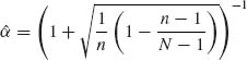 and
and ![]() we get
we get
This is a constant risk (independent of P).
9.1.3
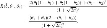
Let w = θ1 + θ2, g(w) = 2w – w2 attains its maximum at w = 1. Thus, R(![]() , θ1, θ2) attains its supremum on {(θ1, θ2): θ1+θ2 = 1}, which is R* (δ) =
, θ1, θ2) attains its supremum on {(θ1, θ2): θ1+θ2 = 1}, which is R* (δ) = ![]() .
.
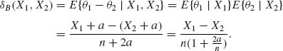
Let ![]() then the Bayes estimator δB(X1, X2) is equal to
then the Bayes estimator δB(X1, X2) is equal to ![]() (X1, X2). Hence,
(X1, X2). Hence,
![]()
Thus, ![]() (X1, X2) is minimax.
(X1, X2) is minimax.
9.1.5
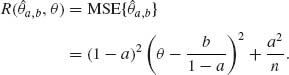
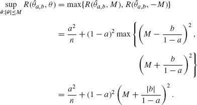
![]()
The value of a that minimizes this supremum is a* = M2/(M2 + 1/n). Thus, if a* = a and b = 0
![]()
Thus, θ* = a* X is minimax.
9.3.3
Θ = {0, 1, 2, …}, L(![]() , θ) = θ (
, θ) = θ (![]() – θ)2.
– θ)2.

The posterior risk is
![]()
Thus, the Bayes estimator is the integer part of
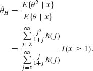
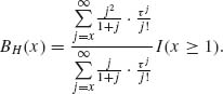
Let p(i;τ) and P(i, τ) denote, respectively, the p.d.f. and c.d.f. of the Poisson distribution with mean τ. We have,
Similarly,
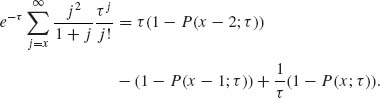
Thus,
![]()
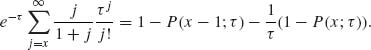
Note that BH(x) > x for all x ≥ 1. Indeed,
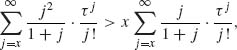
for all x ≥ 1.
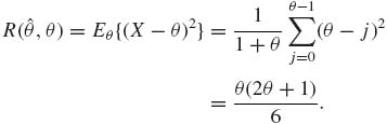
Note that ![]() (θ, 0) = 0. Consider the estimator
(θ, 0) = 0. Consider the estimator ![]() 1 = max(1, X). In this case, R(
1 = max(1, X). In this case, R(![]() 1, 0) = 1. We can show that R(
1, 0) = 1. We can show that R(![]() 1, θ) < R(
1, θ) < R(![]() , θ) for all θ ≥ 1. However, since R(
, θ) for all θ ≥ 1. However, since R(![]() , 0) < R(
, 0) < R(![]() 1, 0),
1, 0), ![]() 1 is not better than
1 is not better than ![]() .
.