CHAPTER 10
Dealing with Circularity
INTRODUCTION
This chapter discusses the issue of dealing with circularities. We make a distinction between circularities that arise as an inherent property of the real-life situation and those resulting from the presence of circular formulae within an implemented model (also called circular references). We discuss the potential advantages and disadvantages of using circular formulae, ways to deal with circular logic and methods to (where desired) retain the inherent circularity in the logic of a real-life situation whilst avoiding any circular formulae in the model.
THE DRIVERS AND NATURE OF CIRCULARITIES
This section discusses the fundamental distinction between circularities that are an inherent property of the real-life situation and those resulting from the way that formulae are implemented in Excel.
Circular (Equilibrium or Self-regulating) Inherent Logic
Many real-life situations can be described using mathematical equations. Often, such equations express some form of equilibrium or self-regulation within a system. For example, the heat generated by a thermostatically controlled radiator depends on the difference between the current room temperature and the target level. At the same time, the room temperature will be affected by (depend on) the new heat generated by the radiator. Similarly, in economics, “circular” logic may arise as a statement of some form of equilibrium within the system being modelled, characterised by the presence of a variable(s) on both sides of some equation(s).
In financial modelling contexts, examples of circular logic include:
- The bonus of senior management could depend on the net income of the company, which is itself calculated net of bonus expense. Written as formulae, one has:
(For simplicity of presentation, we ignore tax; i.e. the bonus may generally be subtracted from pre-tax income.)
- The interest rate at which a company may be able to borrow will depend on the risk that the debt principal and the periodic interest payments may not be able to be met. If the interest-coverage ratio (operating profit divided by interest payment) is used as a measure of this risk, a circularity in logic is created: an increase in the assumed borrowed amount would lead to higher interest charges, a reduced coverage ratio, and hence tend to reduce the amount able to be borrowed (that was just increased). Similarly, for projects financed partially with debt, the debt capacity will depend on the ability to repay the debt, which is linked to the post-tax (and post interest) cash flows, and hence to the level of debt.
- The discount rate used to determine the value of a company (when using the discounted cash flow approach) depends on the company's debt-equity ratio (or debt-to-value ratio). However, a value determined from this approach may initially be inconsistent with the ratios assumed to determine the discount rate, for example if debt levels are regarded as fixed, so that the equity value is a residual that depends on the valuation, meaning that the new implied debt-equity ratio may not be the same as the one that was assumed to derive the value in the first place. The theoretically correct valuation is found only if all assumptions are consistent with each other, which requires an equilibrium (or circular) logic.
- A tax authority may exercise a wealth tax on individuals depending on their net worth, but the net worth is calculated after deducting the wealth taxes.
Circular Formulae (Circular References)
Circular references arise when the calculations to evaluate an Excel cell (or range) involve formulae whose value depends on the same cell or range. This may often occur through a sequence of cell references or formulae, in which the first depends on the last. Such circularities may be intentional or unintentional:
- Unintentional circularities generally result from a mistake or oversight when creating formulae, most often where a model is poorly structured, or has an unclear logical flow (e.g. does not follow the left-to-right and top-to-bottom principle, or uses multiple worksheets with complex linkages between them). A simple example would be if, in Cell B6, a formula such as “=SUM(B4:B6)” had been used in place of “=SUM(B4:B5)”, so that the value in B6 refers to itself.
- Intentional circular references. In principle, these are used to reflect a circular (or equilibrium) logic that is present in the real-life situation. For example:
- Models corresponding to any of the situations described above (i.e. management bonus, cost of debt, debt capacity, cash flow valuation, wealth tax) could potentially be implemented in ways that deliberately contain circular references.
- When calculating period-end cash balances (based on operating income and interest earned during a period), the interest earned within a period may depend on the average cash balance during that period (multiplied by the interest rate). This creates a circular reference, since the average cash balance requires the final balance to be known. In terms of equations, one has:
where Cend is the closing balance, Cbeg is the starting balance, Cop is the non-interest cash inflow and IntRate is the interest rate; the circularity is visible due to the presence of Cend on both sides of the equation.
Generic Types of Circularities
By considering possible combinations of circular logic and circular formulae, one may consider four categories of intentional modelling situations:
- NCL/NCF: No circular logic and no circular formulae. This is the situation for many traditional models: the underlying situation does not require circular logic, and the models also do not contain such logic (apart from unintended errors).
- CL/NCF: Circular logic but no circular formulae. This is where the underlying situation contains a circularity in its logic, but the model ignores this, usually for reasons of simplicity (of implementation) or transparency. Many traditional models fall into this category, such as corporate valuation models, which often ignore circular logic relating to the cost of debt.
- CL/CF: Circular logic and circular formulae. This is where circular formulae are implemented in the model to capture circularity (equilibrium) in the underlying situation. For example, the approach could be used in the contexts cited earlier.
- NCL/CF: No circular logic but circular formulae. Although this category would apparently not exist (except when unintentional circularities arise by mistake), there are cases where the original real-life situation may not be fully circular, but a slight modification to the assumed reality creates circular logic. In fact, the interest calculation described above may be considered to be such a case, since interest is usually not truly paid based on the average balance in a period, but perhaps on interim cash balances at various times throughout a period (so that the assumption that it depends on average balances is a modification to the specification of the reality, that is subsequently captured in the model). In other words, this category is effectively a CL/CF form of this modified reality.
RESOLVING CIRCULAR FORMULAE
In this section, we cover the key methods to deal with potential circular references:
- Correcting the formulae when the circularity results from a mistake or typing error.
- Ignoring the logical circularity, i.e. creating a model which provides only an approximation to, or modification of, the original situation, and in which there is no circularity within the formulae.
- Algebraic manipulation. This involves writing the equations that create the circularity as mathematical formulae, and manipulating them in order to isolate or solve for the (otherwise circular) variables on one side of an equation only. This implicitly retains the equilibrium logic that created the original circularity.
- Using iterative methods, with the aim of finding a stable set of calculations, in which all items are consistent with each other. In practice, this can be achieved by implementing one of several approaches:
- Excel's in-built iterative calculation method, in a model with circular formulae.
- Iterating a “broken” circular path using a VBA macro (or manually conducted copy-and-paste operations).
Correcting Mistakes that Result in Circular Formulae
Clearly, circular formulae that have been implemented by mistake should be removed or corrected. This should be done as soon as they are detected, because it is generally complex to audit completed models to find how the circularity arises: since there is no starting point for a circularity, the tracing of precedents and dependent can become time-consuming and frustrating. It may be that one will need to delete formulae on the circular path and rebuild the model in some way, as an interim step to find and correct the circularity.
Avoiding a Logical Circularity by Modifying the Model Specification
In some cases, a real-life situation may contain circular logic, but it may be possible to ignore this, yet build a model whose accuracy is regarded as sufficient. For example, many corporate valuation models simply ignore the circular logic relating to the discount rate and to the cost of debt. Similarly, for the example concerning ending cash balances, one could eliminate the circularity by assuming that interest is earned on the opening cash balance only:
This approach is simple to implement in practice, but may not be sufficiently accurate in some cases. An improvement in accuracy can be achieved by introducing more sophistication and complexity, in which interest is earned on the total of the opening balance plus the average non-interest cash inflow:
Of course, a reformulation will alter the value of some calculations and outputs, which may or may not be acceptable according to the context. For example, the calculation of the bonus based on pre-bonus income (rather than on post-bonus or net income) would eliminate the circularity. However, the presentation of a result in which the bonus is inconsistent with the final net income figure may not be acceptable or credible (especially since it is a figure which may attract particular attention; an inconsistency in less visible figures may be acceptable).
Eliminating Circular Formulae by Using Algebraic (Mathematical) Manipulation
From a purely mathematical perspective, a formula containing a circularity such as:
can be rearranged to give:
and then solved:
Similarly, in the bonus example:
| i.e. | |
| i.e. | |
| i.e. | |
| and |
Thus, by using the last two formulae in order, the circular references have been eliminated, whilst the underlying circularity of the logic has been retained.
In the calculation of ending cash balances, the circular equation:
can be re-written to isolate Cend on the left-hand side:
| i.e. |
Using the last formula, the ending cash balance can be calculated directly from the starting balance, the interest rate and the non-interest cash flow without creating a circularity. Once Cend is calculated, the interest income can be calculated (also without creating a circularity) as:
Note that when using the algebraic approach, the order of the calculation of the items can be counter-intuitive. For example, using the equations above the bonus is calculated by using the pre-bonus income, and the net income calculated once the bonus is known (which contrasts to the description and formulae at the beginning of the chapter, which defined bonus as a quantity that is determined from net income). Similarly, in the interest calculations, using the formula from algebraic manipulation, the value of Cend is calculated before the interest income, and the interest income is calculated from CEnd, which is counter to the logic that the interest income drives the value of CEnd (or that CEnd depends on interest income).
Resolving a Circularity Using Iterative Methods
The role of a variable that is present on both sides of an equation can often be determined by an iterative solution method (whether working in Excel or more generally). This means that one starts with a trial value (such as zero) for a variable, and this is substituted into one side of the equation (and where the other side is the isolated value of this same variable). For example, with:
using an initial value of B6 as zero on the right-hand side, the process results in the sequence 0, 1, 1.1, 1.11, 1.111. This shows that where a single and stable correct figure exists (i.e. 10/9); iterative methods generally converge very quickly to this.
In theory, an iterative sequence could be explicitly replicated in Excel by building multiple copies of a model, in which the first is populated with trial values, and the outputs of this are used to provide inputs to the second copy, and so on. For example, Figure 10.1 shows the bonus calculations (using a bonus level of 5% of net income). The net income (Cell D5) is determined after subtracting the bonus (Cell D4) from the pre-bonus income figure, and the bonus (Cell D4) itself depends on the net income (Cell D5), thus creating a circular reference. Note that when the circular formula is entered for the first time the result may evaluate to zero (Cell D4). At this point, the figures are not consistent, i.e. the bonus figure as shown is equal to 0% (not 5%) of the net income.

FIGURE 10.1 Example of a Circular Reference Arising from Implementing Equilibrium Logic
In Figure 10.2, we illustrate the iterative process that uses a sequence of models, where the output of each is an input to the next. The values in Row 4 (cells D4:I4) and Row 5 (cells D5:I5) rapidly converge to stable figures that are consistent with each other.

FIGURE 10.2 Illustrative Iterative Process by Using Multiple Copies of a Model
Of course, it is generally not practical to build multiple copies of a model in this way. Rather, iterative methods within the same model are required. There are several possible approaches to doing this, which are discussed in the next section.
ITERATIVE METHODS IN PRACTICE
In practice, iterative methods (for item(s) on a circular path) take the value of a variable at some cell, and calculate the dependent formulae in the circular path, until the original cell has been recalculated, and then the process repeats. This is rather like substituting the value into the “later” parts of the model, until such later parts (due to the circularity) meet the original cell. The general expectation is that the values that are calculated will settle (or “converge”) to stable values which are consistent with each other.
This section discusses three key approaches to the implementation of iterative methods within an Excel model:
- Using Excel's default iterative calculation.
- Using manual iterations of a broken circular path.
- Automating the iterations of a broken circular path using a VBA macro.
Excel's Iterative Method
In the presence of a circular reference, Excel does not have the capability to manipulate the equations or find a correct algebraic solution. Rather, it will use its in-built iterative calculation method, in which the value of a variable at some point on the circular path is used in all dependent formulae, until the original point is reached, giving rise to a new updated value of that variable. This updated value is then used to recalculate the dependent items again, and so on.
The file Ch10.1.BonusCircRef.xlsx contains the bonus model with a circular reference. Figure 10.3 shows the model after applying Excel's iterations (producing results that are the same as in the explicit multi-model approach shown earlier).
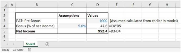
FIGURE 10.3 Results of Allowing Excel to Iterate the Bonus Model Which Contains Circular References
The general presence of a circular reference will be signalled with a “Calculate” message on Excel's Status Bar (as can been seen toward the bottom of Figure 10.3). Further, the Calculation Option settings (under File/Options/Formulas) will have an effect according to the selected option:
- If (the default) Enable Iterative Calculation is switched on:
- On (the default) Automatic calculation method:
- No circular reference warning message will appear when the formula is created.
- The model will directly iterate. The values that result will depend on the number of iterations and the maximum change conditions (that are defined within the calculation options, e.g. the default is to allow 100 iterations).
- The Status Bar will show (using “Calculate”) that there is a circularity present.
- Each further use of the F9 key will result in further iterations being conducted. The model's values will change only if the earlier iterative process has not converged.
- On the Manual recalculation method:
- No circular reference warning message will appear when a formula containing a circular reference is first created.
- The formula will evaluate a single time (i.e. to a context-specific, generally non-zero, value), but it will not iterate beyond this.
- The Status Bar will show (using “Calculate”) that there is a circularity present.
- The use of the F9 key will result in the model performing iterative calculations (with the values that result depending both on the number of iterations and on the maximum change conditions defined in the calculation settings).
- Each further use of the F9 key will result in further iterations being conducted. The model's values will change only if the iterative process has not converged.
- On (the default) Automatic calculation method:
- If Enable Iterative Calculation is switched off:
- On the Automatic calculation method:
- A circular reference warning message will appear when a formula containing a circular reference is first created.
- The formula will evaluate to zero when created or re-entered.
- The Status Bar will explicitly state the presence of a circular reference and indicate the address of one of the cells on the circular path.
- The Excel worksheet will highlight the circularity with precedence and dependence arrows.
- The use of the F9 key will have no further effect on the values in the model, since iterative calculation is switched off, so that the circularity cannot be attempted to be resolved.
- On the Manual recalculation method:
- No circular reference warning message will appear when a formula containing a circular reference is first created.
- The formula will evaluate a single time (i.e. to a context-specific, generally non-zero, value), although the whole model will not evaluate.
- The Status Bar will show that there is a circularity present, but these will not be immediately highlighted with explicit cell references in the Status Bar, nor with precedence and dependence arrows in the Excel worksheet.
- The use of the F9 key will result in a message warning that there is a circular reference. At this point, the Status Bar will also explicitly state the presence of a circular reference and indicate the address of one of the cells on the circular path. The Excel worksheet will highlight the circularity with precedence and dependence arrows. However, there will be no effect on the values in the model, since iterative calculation is switched off, so that the circularity cannot be resolved.
- On the Automatic calculation method:
It is also worth noting that since Excel's default settings (i.e. when first installed) are typically the Automatic and Iterative calculation options (by default), the only indication of a possible circular reference is the presence of “Calculate” in the Status Bar. However, such a message can appear for other reasons (most notably when Excel detects that a model that is set on Manual calculation needs to be recalculated, for example due to a change in the input values used). Thus, the detection of a possible circular reference (e.g. as part of a model auditing process) will need to be done as a deliberate step.
Fortunately, it is simple to detect the presence of a circular reference: by switching off Iterative calculation, a circular reference warning will be displayed, the Status Bar will show the address of a cell on the circular path, and the dependence and precedence arrows appearing in the Excel worksheet. (In Automatic calculation, these will directly appear, whereas in Manual calculation, one will need to press the F9 key for this information to appear.)
Creating a Broken Circular Path: Key Steps
An alternative to using Excel's iterations is to “break” the circular path within the model. This is done by:
- Modifying the model to isolate in a single cell (or in a dedicated range) the value of one variable or calculation that is on the circular path.
- Adding a new cell (or range), whose role is to represent the same variable, but which contains only numbers. The new range may initially be populated with any values (such as zero).
- Relinking the formulae that depend on the original variable, so that they instead depend on the new range. This would need to be done for each formula that is dependent on the original precedent chosen, which is why it is ideal to find or create a precedent with a single dependent if possible. There would then be no more circularity, but there would be two ranges which represent the same variable: the new range (containing pure numbers) and the original range (containing calculated values). Unless the values are the same, the circularity has not been fully resolved.
- Iterate: this means recalculating the model (e.g. pressing F9) and copying the updated values (at each iteration) of the original field into the field containing only numerical values. This can be repeated until the values in each field have converged to the same figure (or the difference between them becomes very small).
The file Ch10.2.Bonus.Iterations.Manual.xlsx contains an implementation of this within the earlier bonus example (see Figure 10.4). Note the process that would have been required if one had started with the model shown in Figure 10.3: first, one would identify that Cell D4 and D5 (in Figure 10.3) are on the circular path, and that D4 has a single dependent. Second, a new range is added (i.e. Row 5 in Figure 10.4). Third, the formulae that are dependent on Cell D4 (i.e. Cell D6 in Figure 10.4, corresponding to Cell D5 in Figure 10.3) are relinked to depend on Cell D5. Fourth, when the model is recalculated, the values of net income (Cell D6) and the calculated bonus (Cell D4) are both updated, as they depend on the values in the new range (Cell D5), rather than on themselves (as was the case with the original circularity). Since the new range (Cell D5) contains only values, there is no longer a circularity.

FIGURE 10.4 Creating a Broken Circular Path
Whilst the process of adapting a model in this way may seem complex at first, in fact it is easy and straightforward to implement if the model is structured in this way as it is being built.
Repeatedly Iterating a Broken Circular Path Manually and Using a VBA Macro
As noted earlier, when iterative processes are convergent, typically only a few iterations are required in order to have stable values. This means that the iterative process can be implemented in several ways:
- Manually pasting the values of the calculated bonus field (Cell D4) into the new bonus value field (Cell D5), ensuring that one recalculates the model after the paste, and repeating this process until one observes sufficient convergence between the figures.
- Implementing a VBA macro to repeatedly assign the values from D4 into D5, also ensuring that the model recalculates each time (repeating this until sufficient convergence has been achieved, which may be checked automatically by the VBA code).
For example, Figure 10.5 shows the result of conducting a single (manual) paste of the values of B4 onto B5 and letting the model recalculate once, whilst Figure 10.6 shows the results of doing this an additional time. Unsurprisingly, the sequence of results produced is the same as that shown for the first steps in Figure 10.2 (i.e. to the values 0, 50, 47.5… , as shown in cells D4, E4 and F4).

FIGURE 10.5 Results After One Paste of the Broken Circular Path Approach

FIGURE 10.6 Results After Two Pastes of the Broken Circular Path Approach
Of course, the manual approach may be sufficient for very simple models which are to be used in only basic ways. However, in practice there are several advantages to using a VBA macro:
- It reduces the chance of an error, especially when repeatedly pasting multi-cell ranges.
- It saves time, since the pressing of a button to run a macro will be quicker than repeatedly copying and pasting ranges, and checking for convergence.
- One is less likely to forget to update the model by recalculating the circularity (indeed, the macro could be automatically run though a workbook open or change procedure, as discussed in Part VI).
- It is easier to run sensitivity analysis, since one can integrate the circular reference macro within a single larger macro (see Chapter 14). The manual procedure would be very cumbersome, as several copy-and-paste procedures would be required each time that an input value is changed.
In Part VI, we describe a simple macro to assign values from one range into another (rather than using copy/paste) which is very straightforward. For example, a code line such as:
Range("BonusValue").Value = Range("BonusCalc").Valuewill perform the assignment (where the Cell D4 has been given the range name BonusCalc and D5 the name BonusValue).
Of course, a recalculation is required after every assignment statement to ensure that the values are updated. Thus, a simple macro that would perform the assignment and recalculate the model several times (here: 10) could be:
Sub MRResolveCirc()For i = 1 To 10Range("BonusValue").Value = Range("BonusCalc").ValueApplication.CalculateNext iEnd Sub
The file Ch10.3.CircRef.BasicMacro.xlsm contains the above macro, and a textbox button has been assigned to run it (see Figure 10.7).

FIGURE 10.7 Resolving a Broken Circular Path Using a Macro
Note that it would be straightforward to add more capability and sophistication, such as using a preset tolerance figure (e.g. 0.00001) and iterating until the difference between the two figures is less than this tolerance, whilst allowing a higher maximum number of iterations if not:
Sub MRResolveCirc2()NitsMax = 100 'Set Max no. of iterationsTol = 0.00001 'Set toleranceicount = 0Do While VBA.Abs(Range("BonusValue).Value - Range("BonusCalc").Value) >= Tolicount = icount + 1If icount <= NitsMax ThenRange("BonusValue").Value = Range("BonusCalc").ValueApplication.CalculateElseExit SubEnd IfLoop
Further, one may display messages to the user if the circularity has not been resolved after a specific number of iterations, as well as error-handling procedures, and so on.
PRACTICAL EXAMPLE
In this section, we show each method within the context of a practical example. We assume that one wishes to forecast a final cash balance based on a starting balance, some non-interest cash flow and interest earned. We discuss the main five possible approaches, as covered earlier:
- Calculating interest income based on average cash balances. This creates a circular logic that may be implemented either with:
- Circular references, resolved using Excel iterations.
- Circular references, resolved using a VBA macro.
- Elimination of the circular references using algebraic manipulation.
- Calculating interest income based on cash balances which exclude non-interest income, thus modifying the model (and its results) to eliminate both the circular logic and the circular references:
- Using starting cash balances only to calculate interest income.
- Using starting balances and non-interest-related cash flows to calculate interest income, thus providing additional accuracy (since the results should be closer to those obtained using circular logic than if only starting cash balances were used).
Using Excel Iterations to Resolve Circular References
The file Ch10.4.1.CircRef.Res.xlsx contains a model in which interest income (Row 5) is calculated by referring to the average of the starting and ending cash balances. Figure 10.8 shows the results after using Excel iterations until the figures are stable.
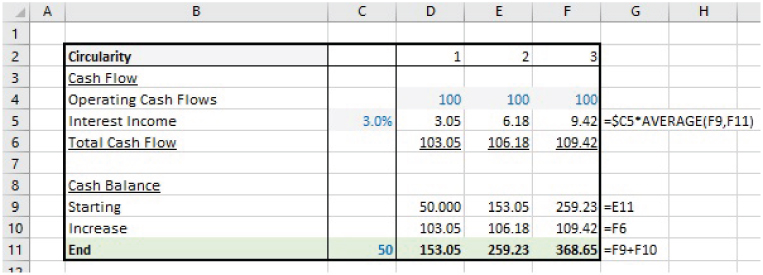
FIGURE 10.8 Using Excel's Iterative Process in a Model with Circular References
Using a Macro to Resolve a Broken Circular Path
The file Ch10.4.2.CircRef.Res.xlsm contains the model with the same underlying logic (interest earned depending on average cash balances), in which a macro is used to resolve a broken circular path (see Figure 10.9). Row 7 contains the pure-values range, so that the macro (at each iteration) copies (assigns) the values from Row 6 into Row 7, until the absolute sum of the differences between the cells in Row 6 and Row 7 (calculated in Cell C8) is within the tolerance level (that is embedded within the macro).

FIGURE 10.9 Using a Macro to Resolve Circular References
Algebraic Manipulation: Elimination of Circular References
The file Ch10.4.3.CircRef.Res.xlsx contains a model in which the formulae (derived earlier in the chapter) resulting from algebraic manipulation are used (see Figure 10.10). Note that, as well as containing no circular references (although the underlying logic remains circular), the order of the calculations is different to those in the original model: the ending cash balance is calculated before the interest income is known, with interest income calculated using the average period cash balance.

FIGURE 10.10 Using Algebraic Manipulation to Eliminate Circular References
Altered Model 1: No Circularity in Logic or in Formulae
An alternative approach is to reformulate the model (and implicitly its specification, in the sense of the assumed or approximated behaviour of the real-world situation), so that there is no circularity of any form.
The file Ch10.4.4.CircRef.Res.xlsx contains the case in which interest income is determined from starting cash balances only. This removes the circularity, as interest earned no longer depends on ending cash balances (see Figure 10.11). Note that the values of the ending cash balances are different to the above examples in which circularity was retained.

FIGURE 10.11 Altering the Model to Eliminate Circularity Using Starting Balances
Altered Model 2: No Circularity in Logic in Formulae
Another approach to reformulate the model would be to calculate interest income from starting cash balances as well as from all other (non-interest) cash sources. This would also eliminate the circularity, whilst potentially giving results that are closer to those that would be obtained if the circularity were retained.
The file Ch10.4.5.CircRef.Res.xlsx contains such a model (see Figure 10.12). Note that the values of the ending cash balances are much closer to those in the earlier examples which used circularity.

FIGURE 10.12 Altering the Model to Eliminate Circularity Using Starting Balances and Interim Non-interest Cash Flows
Note that in this example, the only non-interest cash flow is the single line for the operating income. In a larger model, one may wish to include all non-interest cash items (including capital investment, dividends or financing cash flows). Doing so can be a little cumbersome in practice, because one needs to create a partially complete cash flow statement, which includes all non-interest-related cash items. Sometimes a convenient compromise is to include only the major cash flow items in such a statement, where the identity of the larger items can be known in advance.
SELECTION OF APPROACH TO DEALING WITH CIRCULARITIES: KEY CRITERIA
When faced with a situation in which there is a potential for circular references, one has a choice as to which approach to use, not only in terms of their incorporation into a model, but also in the methods used to resolve them. This section discusses some key issues to consider when making such a choice.
Currently, there seems to be very little consensus or standardisation around whether and/or how to use circularities:
- Some modellers take the view that circular references should be avoided at all costs.
- Some modellers (especially some practitioners of financial statement modelling and of project finance modelling) seem to place significant value on retaining circular references in the calculations, typically for the sake of accuracy and consistency.
- Some modellers prefer to ignore the circular logic of a situation when building models, including many valuation practitioners, as mentioned earlier in the chapter.
Although the reasons to use (or to avoid) circularities are often not addressed explicitly, there is surely some underlying rationale for many of these views, which manifests itself differently according to the context, and the modeller's experience, capabilities and biases. Indeed, there are several issues to consider when selecting an approach to deal with potential circularities:
- The accuracy and validity of the underlying logic.
- The complexity and lack of transparency of the model.
- The potential for errors due to iterative processes to not converge to a stable figure, but to diverge or float in ways that may not be evident.
- The risk of destroying calculations by the propagation of non-numerical errors along the circular path, without any easy possibility to correct them.
- The possibility that macros may be poorly written, not robust, or contain errors (especially when written by modellers with insufficient experience with VBA).
- That mistakes may be made when performing algebraic manipulation, resulting in incorrect calculations.
- That calculation speed may be compromised.
- That sensitivity analysis may be more cumbersome to conduct that in models without circularity.
These issues are discussed in detail in the remainder of the text.
Model Accuracy and Validity
Where a real-life situation involves circular (equilibrium) logic, it would seem sensible to capture this. On the other hand, although the economic concept of equilibrium is widely accepted, the notion of “circular reasoning” is generally regarded with suspicion. Thus, in some cases, one may be willing to reduce accuracy in order to retain more confidence:
- Where there is a strong need for the calculations to be as accurate as possible, and (internally) consistent, one may essentially be obliged to accept that circular logic is required. For example, typically in project finance modelling, the debt covenants or other contractual aspects may be set with reference to the figures in a model. Similarly, in the earlier bonus example, if the bonus net income figures are not consistent, then these may not be credible and are technically also wrong. In such cases, one's options are either to use algebraic manipulation (where possible) or to use iterative methods with Excel or VBA.
- Where the requirements for accuracy or consistency may be less strict, or circular logic may be distrusted per se, it may be sufficient (or preferable) to ignore the circular logic. The reduced accuracy may be acceptable either because the results are not materially affecting (e.g. in most interest calculations when this is only a small part of the overall cash flow) and/or simply because ignoring the circularity has become standard practice in a specific context (as is the case in some valuation work).
Note that in principle, the use of algebraic manipulation provides the best of both worlds: retaining the implicit circular logic whilst not having circular formulae. Unfortunately, there are some limitations and potential drawbacks:
- In practice, it can be used only in a limited set of specific and simple situations. Many real-life modelling situations typically contain calculations that are too complex (or impossible) to be manipulated algebraically. For example, even the relatively minor change of introducing multiple interest rates (that apply depending on the cash balance) would mean that manipulations similar to those shown earlier are no longer possible (due to the presence of IF or MIN/MAX statements in the equations).
- Even where appropriate manipulations are possible, there is generally no easy way to know if a mistake has been made when doing so. To check the results of implementing the manipulated formulae with those that would be achieved if the original formulae had been used, one would have to implement both (and the original formulae would then contain circular references which would need to be resolved by an iterative method).
- Users of a model who are not familiar with the approach may find it hard to understand. Not only would they not be explicitly aware of the underlying algebraic manipulation (unless it is made very clear in the model documentation or comments), but also the corresponding Excel formulae are generally less clear. Further, the order of the calculations is sometimes also not intuitive and confusing (e.g. ending cash balances calculated before the interest income).
Complexity and Transparency
Models with circular references are hard and time-consuming to audit (and even more so in multi-sheet models). The circular dependency path literally leads one to moving in circles when trying to understand the formulae and check their accuracy; after trying to follow the logic along a calculation path, one eventually simply returns to where one started, often without having gained any new useful information! In addition, some users may be insufficiently familiar with, and distrust, iterative processes per se. Finally, the potential requirement to use macros to run iterative processes can lead to further unwillingness to consider the use of circularity.
In terms of implications for choice of method, this suggests that:
- The use of circular formulae should be avoided whenever possible.
- Where circular logic (without circular formulae) is desired to be retained:
- The use of a “broken” circular path (combined with a macro to conduct the required iterations) can be an appropriate way to retain the circular/equilibrium logic (and hence the accuracy of the model) whilst having clear dependency paths (with definite start and end points).
- The use of algebraic manipulation (where available) is not necessarily more transparent (nor less complex) than the use of a broken circular path, since users who are not familiar with (or capable of understanding) the mathematical manipulations may find the model harder to follow.
- The use of alternative modelling approaches may overcome any complexity associated with the need to use iterative processes. However, the complexity of the model will not be significantly reduced, since the alternative model and the broken-path model would be of similar transparency and complexity in principle. The disadvantage of using an alternative modelling approach is the reduced accuracy compared to if a broken circular path (or circular formulae) were used.
Non-convergent Circularities
The use of iterative methods can have negative consequences for the robustness of a model, and the extent to which the displayed results are meaningful and converge to the correct values.
In fact, whilst the general expectation when using iterative processes is that they will converge, this will not necessarily be the case. In fact, iterative processes may be either:
- Convergent
- Divergent
- Floating.
For example, we noted earlier that an iterative process applied to a formula such as:
converged after only a few iterations (to the true figure of 10/9).
On the other hand, whilst it is clear that the formula
has the true (mathematical) solution B6=−1, an iterative method (using an initial value of zero) would produce the rapidly divergent sequence: 0, 1, 3, 7, 15, 31, 63, 127, 255, 511, 1023….
In fact, just as iterative processes converge quickly (where they are convergent), they also diverge quite quickly (where they are divergent). Thus, the presence of divergent circularities will typically be evident, unless only very few iterations are used.
The file Ch10.5.1.CircRef.Res.xlsx contains an example of the earlier interest-calculation model in which there is a circular reference. For ease of presentation, the file contains a second copy of the model (see Figure 10.13). In the second copy, the interest rate has been set to 200% (Cell C16). At this or any higher value, the iterative process will diverge. Since (in Excel) the number of iterations is 100 by default, the numbers shown are large, but not yet very large. Each pressing of F9 results in 100 additional iterations, so that the figures become progressively larger.

FIGURE 10.13 Example of a Divergent Circular Reference
Such divergent behaviour (when the interest rate is 200% or higher) results from the circularity in the logic (not just the specific model, as implemented here): the interested reader can verify that the divergence will occur (or errors or incorrect results produced), whether a macro is used to iterate, or whether algebraic manipulation is used. The alternative models (in which interest earned is not linked to ending cash balances) do not have these properties.
Circularities that are neither divergent nor convergent can exist; we call these “floating circularities”. For example, whereas the equations:
have the solution ![]() , an iterative process applied to the Excel cells with the formulae:
, an iterative process applied to the Excel cells with the formulae:
will produce a sequence of floating values for D3 and E3, i.e. they cycle through a set of values, without ever converging or diverging. The values will depend on the number of iterations used and on the assumed or implied starting values (of say D3) at the first iteration (i.e. which point in the cycle one looks at).
The file Ch10.6.1.CirRef.Floating.xlsx contains an example. The file is set to Manual recalculation, with iterative calculation on, and set to only one iteration (thus, each pressing of F9 will result in a single iteration). Figure 10.14 shows the results of conducting one iteration, Figure 10.15 shows the result of conducting two, and Figure 10.16 shows the result of conducting three. The floating nature of the circularity can be seen as the values in Figure 10.16 are the same values as those in Figure 10.14, whilst those in Figure 10.15 are different.

FIGURE 10.14 The Result of One Iteration with a Floating Circularity

FIGURE 10.15 The Result of Two Iterations with a Floating Circularity

FIGURE 10.16 The Result of Three Iterations with a Floating Circularity
The non-convergent nature of the calculations (and the different results that are possible) can be seen in more detail from the lower part of the file, shown in Figure 10.17. This shows the explicit iterative steps, from an assumed value of D3 at the beginning of the iterative process (Cell D7). The user can verify that the sequence generated is different if an alternative starting value is used.
FIGURE 10.17 The Values of Each Item at Each Iteration with a Floating Circularity
Floating circularities can arise in subtle ways, for reasons that may not be immediately apparent. For example, one may start with a calculation of all future cash sources, uses and cash balances, with the forecast showing that future balances are always positive, as shown in Figure 10.18. One may then to decide to add an additional draw-down line item, in which, at the beginning of the project, the minimum future cash balance is withdrawn (e.g. so that this cash can immediately be used for other purposes). In other words, Cell C3 is replaced by a formula which calculates the (negative of) the minimum of the range D4:H4 (see Figure 10.19, which shows both models for simplicity). This will create a “floating” circularity: as soon as cash is drawn down, the future minimum balance becomes zero, so that no future cash can be drawn down, which then resets the future minimum cash balance to a positive number, so that cash can be drawn down after all, and so on.

FIGURE 10.18 Initial Forecast Model

FIGURE 10.19 Modified Forecast Model with a Floating Circularity
Floating circularities are arguably the most dangerous type:
- Since they do not diverge, the values shown may look reasonable. However, the values are not stable, and depend on the number of iterations used.
- Their cause is often subtle, so one may not be conditioned to be aware of their possible presence.
- Their presence may be overlooked, especially if intentional (convergent) circularities are also used. The main risk is that a floating circular reference will unintentionally be introduced, yet the modeller (or user) is likely to ignore any circular reference warning messages in Excel (because a circular reference was used intentionally).
The main implication is that, if using Excel's iterative method, there is a risk that inadvertent floating circularities may be introduced inadvertently or be hidden by other intentional circularities. To avoid this, in principle, Excel's iterative method should not be used.
Potential for Broken Formulae
In models with circular formulae, errors may propagate along the circular path, without any easy mechanism to correct them. This can cause significant problems: in the best case, one would have to revert to a prior saved version of the file. In the worst case, one may have inadvertently saved the model with such errors in (or such errors are only propagated at the recalculation that may take place automatically when a file is saved), with the result that the model is essentially destroyed and may have to be rebuilt.
The issue arises because once a non-numerical error value (such as #DIV/0!) is introduced onto the circular path, then the iterative process will propagate it. However, if the error is corrected at only one cell on the path, the iterative process will not generally be able to recover, because some of the other cells on the path will contain non-numerical errors, so that the iterative calculation process (which requires pure numerical values as inputs) simply cannot be conducted.
Figure 10.20 shows the earlier circular calculation of interest earned (i.e. depending on average cash balances), in which the periodic interest rate had been set to 250% and the model iterated several times. Since the circularity is divergent, eventually the #NUM! error appears on cells along the circular path.

FIGURE 10.20 Initial Error Propagation due to a Divergent Circularity
Figure 10.21 shows the result of replacing the 250% interest rate to a periodic rate of 3%, and iterating the calculations several times. One can see that the formulae on the circular path are not corrected.

FIGURE 10.21 Errors Remaining After Correction of the Cause of the Divergent Circularity
In Figure 10.22, we show that even when the formulae are re-entered across Row 5, and the iterations conducted, the model remains broken. The same is true if formulae are entered in Row 6 or Row 10.

FIGURE 10.22 Errors Remaining After Partial Rebuild of Model Formulae
In fact, only in the case in which the formulae are entered all the way to Row 11, are the formulae re-established, and then only in the first column (see Figure 10.23). Thus, to recover the model, one would need rebuild it at Row 11, progressing from left to right, one cell at a time (by re-entering the formula in each cell and then iterating or recalculating the model).

FIGURE 10.23 Successful Rebuild of One Column of the Model
Many practical models (which are mostly larger and often do not have a strict left-to-right flow) would be essentially impossible to rebuild in this way; therefore, the potential arises to essentially destroy the model.
Note that such a problem is much simpler to deal with in a model that has been built with a broken circular path: when an error such as the above arises, the pure-values field that is used to break the circular path will be populated with the error value (e.g. #NUM!). These can be overwritten (with zero for example), in addition to correcting the input value that caused the error or divergence. Since there is no circularity in the formulae, once the contents of the values field are reset from the error value to any numerical value, the dependent formulae can all be calculated and reiterated without difficulty.
Figure 10.24 shows the earlier model with a broken circular path, iterated to the point at which the #NUM! errors occur, and Figure 10.25 shows the result of correcting in model input (periodic interest, in Cell C5), overwriting the #NUM! errors in Row 7 with zeros, and performing the iterations.
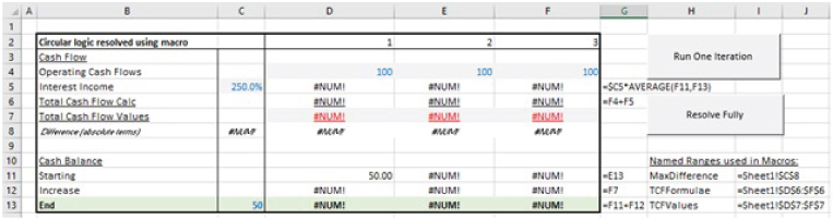
FIGURE 10.24 Errors in a Model with a Broken Circular Path

FIGURE 10.25 Simple Process to Correct Errors in a Model with a Broken Circular Path
The main implication is that the use of a broken circular path is preferable to the use of Excel iterations, if one is to avoid the potential to destroy models or create significant rework.
Calculation Speed
Since each iteration is a recalculation, the use of iterative processes will result in longer calculation times in similar models in which iterations are not necessary (i.e. one without circular formulae). Further, it is likely that in general, Excel iterations would be quicker than the use of a VBA macro, simply because Excel's internal calculation engine is highly optimised (and hence difficult for a general programmer to surpass in performance).
The main implication is that, from the perspective of speed, circular formulae are less efficient (so that algebraic manipulation or modified models without circular formulae would be preferred), and that, where circular formulae are required, the use of VBA macros is generally slightly less computationally efficient than the use of Excel's iterations.
Ease of Sensitivity Analysis
For models in which there is a dynamic chain of calculations between the input and outputs (whether involving circular formulae or not), Excel's DataTable sensitivity feature can be powerful (see Chapter 12). The introduction of a macro to resolve circular references will inhibit the use of this, meaning that macros would also be required to conduct sensitivity analysis in this case (see Chapter 14).
The main implication is that, from the perspective of conducting sensitivity analysis, the use of broken circular paths is more cumbersome than the use of the other methods.
Conclusions
The overall conclusions of the discussion in this section are:
Where there is circular logic that is inherent in a situation, one should consider whether it is genuinely necessary to capture this within the model (for accuracy, presentation or consistency purposes), or whether an alternative sufficiently accurate approach (which has no circular logic) can be found. In such a case, the models can be built using standard techniques (i.e. without requiring macros or iterative methods), with such models calculating quickly and allowing for standard sensitivity analysis techniques to be employed. Clearly, where this is possible, it should be the preferred approach.
Where it is necessary to capture the effect of circular logic within the model, several methods can be considered:
- Algebraic manipulation. This will avoid any circular formulae, whilst nevertheless creating a model that captures the circular logic. The model will not require iterative methods, will calculate efficiently, and allow for sensitivity analysis to be conducted (using Excel DataTables). Disadvantages include the very small number of cases where it is possible to do the required manipulations, the possibility of mistakes made during the manipulation (since to check the result would require implementing an alternative model which contains circular references), and that the transparency of the model may be slightly reduced (since the manipulations may not be clear to some users, and the order of the calculation of some items is changed and may not be intuitive).
- Excel iterations. This allows the retention of sensitivity analysis using DataTables and is more computationally efficient than using macros to iterate the circularity. The most significant disadvantages include:
- The difficulty in auditing the model.
- The potential for a floating circularity to not be detected, so that the model's values may be incorrect.
- The potential to damage the model and to have to conduct significant rework.
- The process by which Excel handles iterations may not be clear to a user, as it is neither transparent nor very explicit.
- Breaking the circularity and iterating. The advantages of this are significant, and include:
- The model is easier to audit, as there is a (standard) dependency route (with a beginning and an end).
- One is in explicit control of the circularity, so that inadvertent (floating) circular references (which may create incorrect model values) are easy to detect, because any indications by Excel that a circular reference is present will be a sign of a mistake in the formulae.
- The process to correct a model after the occurrence of error values is much simpler.
- The main disadvantages compared to the use of Excel's iterative method include the need to write a macro, the slightly more cumbersome process to run a sensitivity analysis, and a slightly reduced computational efficiency.
In the author's view, the overall preference should be to avoid circularity by model reformulation if possible (where accuracy can be slightly compromised), then to explore possible algebraic approaches, and otherwise to use a macro to resolve a broken circular path. Excel's iterative method should essentially not be used.