Chapter 13
Examples of Regular Surfaces
This chapter provides worked examples of graphs of functions in ![]() and
and ![]() , and surfaces of revolution in
, and surfaces of revolution in ![]() . The details of computations, which are not included, are based on formulas appearing in Theorems 12.10.1–12.10.4. In this chapter, we identify ℝ2
with the
xy
‐plane in ℝ3
. See Example 12.8.6 for a summary of Gauss curvatures as well as related comments.
. The details of computations, which are not included, are based on formulas appearing in Theorems 12.10.1–12.10.4. In this chapter, we identify ℝ2
with the
xy
‐plane in ℝ3
. See Example 12.8.6 for a summary of Gauss curvatures as well as related comments.
Each of the regular surfaces to be considered can be parametrized as either the graph of a function or a surface of revolution. The former approach has the advantage that the regular surface can be depicted literally as a graph in ℝ3 . On the other hand, when symmetries are present, the surface of revolution parametrization can be quite revealing and computationally convenient. The choice of parametrization made here is somewhat arbitrary. There is a small issue that differentiates the two computational methods. Parameterizing a regular surface as a surface of revolution leaves out certain points compared with the corresponding parametrization as the graph of a function; more specifically, with the former approach, part of a longitude curve is “missing”. Since we are interested exclusively in local aspects of regular surfaces, in particular, the Gauss curvature, this is not a concern and will not be discussed further.
13.1 Plane in 
The set
is the xy ‐plane in ℝ3 . In the notation of Theorem 11.4.2, let
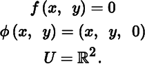
By Theorem 11.4.2, Pln is a regular surface and (U, φ) is a chart. Viewing Pln as a regular surface in ![]() , Theorem 12.10.1 gives:
, Theorem 12.10.1 gives:

13.2 Cylinder in 
The set
is an infinite cylinder standing on the xy ‐plane in ℝ3 . In the notation of Theorem 11.4.3, let

By Theorem 11.4.3, Cyl is a regular surface and (U, φ) is a chart. Viewing Cyl as a regular surface in ![]() , Theorem 12.10.3 gives:
, Theorem 12.10.3 gives:

An intuitive explanation for why the Gauss curvature of Cyl equals 0 is given in Example 12.8.6.
13.3 Cone in 
The set
is an inverted infinite cone (minus its vertex) standing on the xy ‐plane in ℝ3 . See Figure 13.3.1.
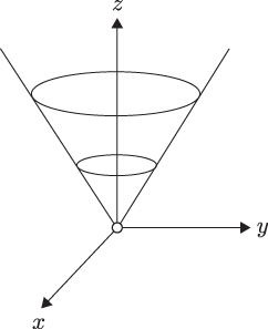
Figure 13.3.1. Con
In the notation of Theorem 11.4.3, let

By Theorem 11.4.3, Con is a regular surface and (U, φ) is a chart. Had the vertex (0,0,0) been included as part of Con, the resulting set would not be a regular surface because there is more than one tangent plane at (0,0,0).Viewing Con as a regular surface in ![]() , Theorem 12.10.3 gives:
, Theorem 12.10.3 gives:

An intuitive explanation for why the Gauss curvature of Con equals 0 is given in Example 12.8.6.
13.4 Sphere in 
For a real number R > 0, the set
is a sphere of radius R centered at the origin. See Figure 13.4.1.


When
R = 1, we write ![]() in place of
in place of ![]() . In the notation of Theorem 11.4.3, let
. In the notation of Theorem 11.4.3, let

By Theorem 11.4.3, ![]() is a regular surface and (U, φ) is a chart. Viewing
is a regular surface and (U, φ) is a chart. Viewing ![]() as a regular surface in
as a regular surface in ![]() , Theorem 12.10.3 gives:
, Theorem 12.10.3 gives:

When
R = 1, we have ![]() ; that is,
; that is, ![]() for all (θ, ϕ) in
U
. This is consistent with Theorem 12.2.12(c).
for all (θ, ϕ) in
U
. This is consistent with Theorem 12.2.12(c).
13.5 Tractoid in 
The set

is the upper portion of the tractoid, also known as the tractricoid. It is better understood as the surface obtained by revolving around the z ‐axis the smooth curve σ(t) : (0, + ∞) → ℝ3 given
See Figure 13.5.1. In the notation of Theorem 11.4.3, let

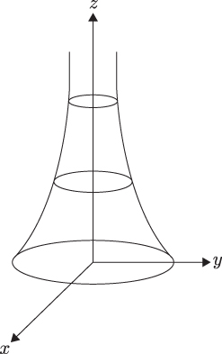
Figure 13.5.1. Trc
By Theorem 11.4.3, Trc is a regular surface and (U, φ) is a chart. Viewing Trc as a regular surface in ![]() , Theorem 12.10.3 gives:
, Theorem 12.10.3 gives:
Together with Pln and ![]() , Trc makes a trio of regular surfaces in
, Trc makes a trio of regular surfaces in ![]() with constant Gauss curvatures of 0, 1, and −1, respectively.
with constant Gauss curvatures of 0, 1, and −1, respectively.
13.6 Hyperboloid of One Sheet in 
The set
is the upper half of a hyperboloid of one sheet. See Figure 13.6.1.

Figure 13.6.1.
One, 
In the notation of Theorem 11.4.2, let

By Theorem 11.4.2, One is a regular surface and (U, φ) is a chart. Viewing One as a regular surface in ![]() , Theorem 12.10.1 gives:
, Theorem 12.10.1 gives:

We observe that the Gauss curvature is nonconstant and strictly negative.
13.7 Hyperboloid of Two Sheets in 
The set
is the upper sheet of a hyperboloid of two sheets. See Figure 13.7.1. In the notation of Theorem 11.4.2, let
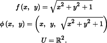

Figure 13.7.1. Two, ℋ2
By Theorem 11.4.2, Two is a regular surface and (U, φ) is a chart. Viewing Two as a regular surface in ![]() , Theorem 12.10.1 gives:
, Theorem 12.10.1 gives:

We observe that the Gauss curvature is nonconstant and strictly positive.
13.8 Torus in 
For a real number R > 1, the set

is the torus obtained by rotating about the z ‐axis the unit circle in the xz ‐plane centered at (R, 0, 0). See Figure 13.8.1.

Figure 13.8.1. Tor
In the notation of Theorem 11.4.3, let
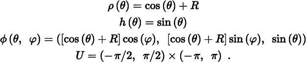
The domain for
h
was chosen to be (−π/2, π/2) instead of (0, 2π), for example, to ensure that property [R2] of Section 11.4 is satisfied. This parametrizes the “outer” half of the torus; a separate parametrization gives the “inner” half. It follows from Theorem 11.4.3 that Tor is a regular surface and (U, φ) is a chart. Viewing Tor as a regular surface in ![]() , Theorem 12.10.3 gives:
, Theorem 12.10.3 gives:

As depicted in Figure 13.8.1, the Gauss curvature takes positive, negative, and zero values at various points of Tor.
13.9 Pseudosphere in 
The set
is the same upper half of the hyperboloid of one sheet described in Section 13.6, and just as before, it is a regular surface. Since
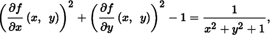
the condition of Theorem 12.2.8 is satisfied. Thus, ![]() is a regular surface in
is a regular surface in ![]() . Alternatively, this comes directly from Theorem 12.2.12(a). Theorem 12.10.2 gives:
. Alternatively, this comes directly from Theorem 12.2.12(a). Theorem 12.10.2 gives:

We note that ![]() agrees with Theorem 12.2.12(d). In the context of
agrees with Theorem 12.2.12(d). In the context of ![]() , we refer to
, we refer to ![]() as the pseudosphere.
as the pseudosphere.
13.10 Hyperbolic Space in 
The set
is the same upper sheet of the hyperboloid of two sheets described in Section 13.7, and just as before, it is a regular surface. Since

and, by definition,
x
2 + y
2 > 1, the condition of Theorem 12.2.8 is satisfied. Thus, ℋ2
is a regular surface in ![]() . Alternatively, this comes from directly from Theorem 12.2.12(a). Theorem 12.10.2 gives:
. Alternatively, this comes from directly from Theorem 12.2.12(a). Theorem 12.10.2 gives:

We note that ![]() agrees with Theorem 12.2.12(d). In the context of
agrees with Theorem 12.2.12(d). In the context of ![]() , we refer to ℋ2
as hyperbolic space.
, we refer to ℋ2
as hyperbolic space.
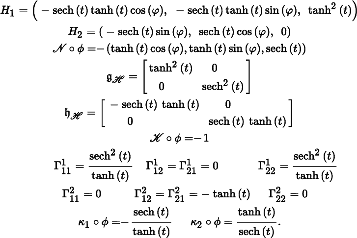
We can also parametrize ℋ2 as a surface of revolution. In the notation of Theorem 11.4.3, let
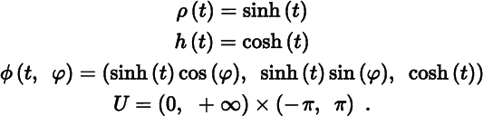
From the well‐known identity sinh2(t) − cosh2(t) = − 1, we obtain ![]() . Evidently, the condition of Theorem 12.2.9 is satisfied, so once again we see that ℋ2
is a regular surface in
. Evidently, the condition of Theorem 12.2.9 is satisfied, so once again we see that ℋ2
is a regular surface in ![]() . Theorem 12.10.4 gives:
. Theorem 12.10.4 gives:

We observe from ![]() that the coordinate frame ℋ is orthogonal, giving this parametrization certain computational advantages.
that the coordinate frame ℋ is orthogonal, giving this parametrization certain computational advantages.